2
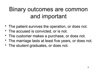
Binary outcomes arecommon
and important
• The patient survives the operation, or does not.
• The accused is convicted, or is not.
• The customer makes a purchase, or does not.
• The marriage lasts at least five years, or does not.
• The student graduates, or does not.
5
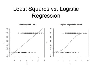
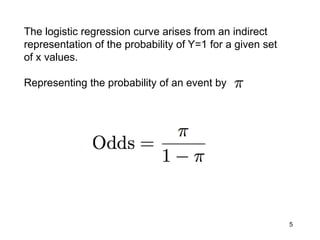
The logistic regressioncurve arises from an indirect
representation of the probability of Y=1 for a given set
of x values.
Representing the probability of an event by
6.
6
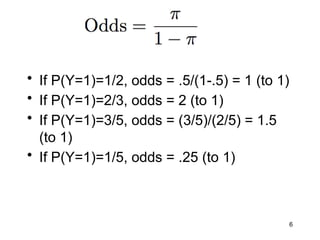
• If P(Y=1)=1/2,odds = .5/(1-.5) = 1 (to 1)
• If P(Y=1)=2/3, odds = 2 (to 1)
• If P(Y=1)=3/5, odds = (3/5)/(2/5) = 1.5
(to 1)
• If P(Y=1)=1/5, odds = .25 (to 1)
10
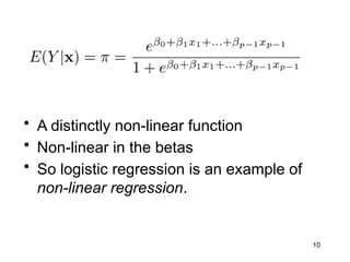
• A distinctlynon-linear function
• Non-linear in the betas
• So logistic regression is an example of
non-linear regression.
11.
11
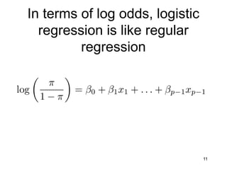
In terms oflog odds, logistic
regression is like regular
regression
12.
12
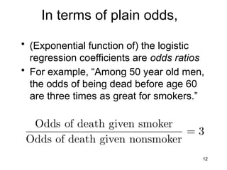
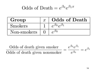
In terms ofplain odds,
• (Exponential function of) the logistic
regression coefficients are odds ratios
• For example, “Among 50 year old men,
the odds of being dead before age 60
are three times as great for smokers.”
13.
13
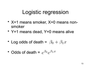
Logistic regression
• X=1means smoker, X=0 means non-
smoker
• Y=1 means dead, Y=0 means alive
• Log odds of death =
• Odds of death =
17
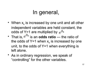
In general,
• Whenxk is increased by one unit and all other
independent variables are held constant, the
odds of Y=1 are multiplied by
• That is, is an odds ratio --- the ratio of
the odds of Y=1 when xk is increased by one
unit, to the odds of Y=1 when everything is
left alone.
• As in ordinary regression, we speak of
“controlling” for the other variables.
18.
18
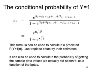
The conditional probabilityof Y=1
This formula can be used to calculate a predicted
P(Y=1|x). Just replace betas by their estimates
It can also be used to calculate the probability of getting
the sample data values we actually did observe, as a
function of the betas.
20
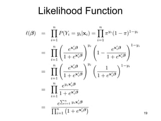
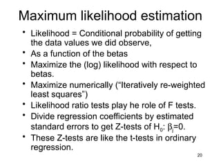
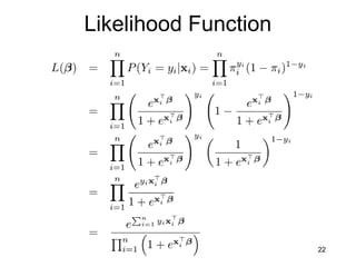
Maximum likelihood estimation
•Likelihood = Conditional probability of getting
the data values we did observe,
• As a function of the betas
• Maximize the (log) likelihood with respect to
betas.
• Maximize numerically (“Iteratively re-weighted
least squares”)
• Likelihood ratio tests play he role of F tests.
• Divide regression coefficients by estimated
standard errors to get Z-tests of H0: bj=0.
• These Z-tests are like the t-tests in ordinary
regression.
21.
21
The conditional probabilityof Y=1
This formula can be used to calculate a predicted
P(Y=1|x). Just replace betas by their estimates
It can also be used to calculate the probability of getting
the sample data values we actually did observe, as a
function of the betas.
23
Copyright Information
This slideshow was prepared by Jerry Brunner, Department of
Statistics, University of Toronto. It is licensed under a Creative
Commons Attribution - ShareAlike 3.0 Unported License. Use
any part of it as you like and share the result freely. These
Powerpoint slides will be available from the course website:
http://www.utstat.toronto.edu/brunner/oldclass/302f14
Editor's Notes
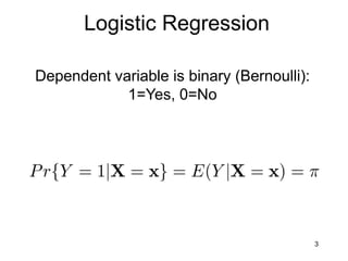
#3 Data analysis text has a lot of this stuff
Pr\{Y=1|\mathbf{X}=\mathbf{x}\} = E(Y|\mathbf{X}=\mathbf{x}) = \pi % 36
#8 Beta0 is the intercept.
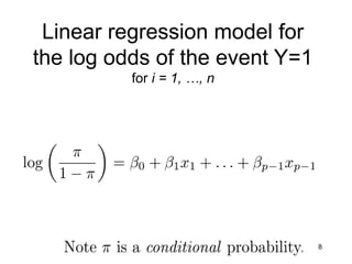
$\beta_k$ is the increase in log odds of $Y=1$ when $x_k$ is increased by one unit,
and all other explanatory variables are held constant.
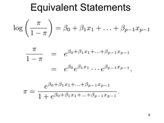
\begin{equation*}
\log\left(\frac{\pi}{1-\pi} \right) =
\beta_0 + \beta_1 x_1 + \ldots + \beta_{p-1} x_{p-1}.
\end{equation*} % 32
Note $\pi$ is a \emph{conditional} probability. % 32


![logistic model final_pptx__corected_one[1].pptx](https://cdn.slidesharecdn.com/ss_thumbnails/finalpptxcorectedone1-251124022241-c29356b7-thumbnail.jpg?width=640&height=640&fit=bounds)