Download as PDF, PPTX


![Notations
Let the time interval be fixed [0, T]. Let τi be time to default for obligor i.
Let Yi = 1τi ≤T be the default indicator.
Then, we can represent the probability of default for obligor i as,
PDi = P(Yi = 1) = 1 − P(Yi = 0) = P(τi ≤ T) (1)
Let EADi be the exposure at default and LGDi be the loss given default.
Then the default loss on a porfolio is,
Default Loss =
n
i=1
EADi × Yi × LGDi (2)
Since Yi is a Bernoulli r.v., E[Yi ] = PDi . This gives us the Expected value
of the default loss. However, we are interested in different quantiles of the
loss distribution function.
Mital, Swati (PRMIA) Credit Default Models May 4, 2016 4 / 31](https://image.slidesharecdn.com/creditdefaultmodelsexternal-160504190001/85/Credit-Default-Models-4-320.jpg)

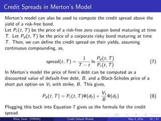
![Diagrammatic Representation
Figure: Merton Structural Model (source: Crouhy et al., A comparative analysis
of current credit risk models, Journal of Banking and Finance, 2000 [59-117])
Mital, Swati (PRMIA) Credit Default Models May 4, 2016 8 / 31](https://image.slidesharecdn.com/creditdefaultmodelsexternal-160504190001/85/Credit-Default-Models-8-320.jpg)

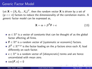
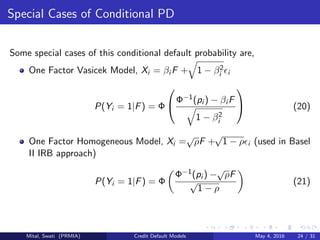
![Multivariate Firm Value Model
Here we extend Merton’s ideas into something that can be used on a large
portfolio by using factors for modelling dependence.
Consider a portfolio of n firms over a time period [0, T]. Assume
T = 1.
Let Yi denote default indicator. So, Yi = 1 indicates that a default
event has taken place and Yi = 0 means there is no default.
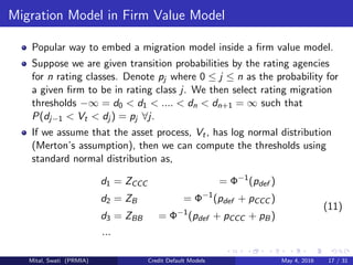
The default of the company is driven by some latent variable Xi ,
generally assumed to be normally distributed, which if it lies below a
threshold di , a default occurs. Therefore, we can write the default
probability as,
P(Yi = 1) = P(Xi ≤ di ) = F(di ) (12)
Model default dependence between the different firms in the portfolio
by making the Xi correlated, i.e., to make the asset values dependent.
Mital, Swati (PRMIA) Credit Default Models May 4, 2016 18 / 31](https://image.slidesharecdn.com/creditdefaultmodelsexternal-160504190001/85/Credit-Default-Models-18-320.jpg)

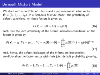
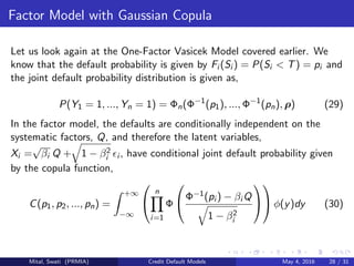
![Copulas
Definition
Let C be a copula function. Then C : [0, 1]n → [0, 1] such that there are
random variables U1, U2, ..., Un that take values on [0, 1] whose joint
cumulative distribution function is C.
C(u1, u2, ..., un) = P(U1 ≤ u1, U2 ≤ u2, ..., Un ≤ un) (22)
Multivariate Distribution using Copula
Consider a vector of random variables (X1, X2, ..., Xn) such that their
univariate marginal distribution functions are (F1(x1), F2(x2), ..., Fn(xn)).
Then the Copula function results in their multivariate joint distribution,
C(F1(x1), F2(x2), ..., Fn(xn)) = F(x1, x2, ..., xn) (23)
Sklar’s Theorem established that any multivariate distribution F can be
written in this form using a Copula Function.
Mital, Swati (PRMIA) Credit Default Models May 4, 2016 25 / 31](https://image.slidesharecdn.com/creditdefaultmodelsexternal-160504190001/85/Credit-Default-Models-25-320.jpg)

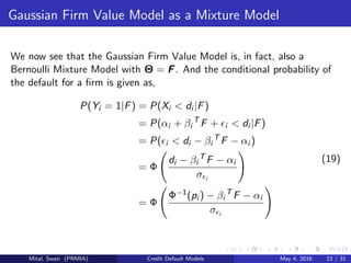
![Default Correlation Models
Modelling default dependence for credit portfolios using Copulas was
popularized by Li in [2]. We build our framework with the following
assumptions.
We have n firms and we want to model their default correlations over
a fixed time period [0, T].
We have the marginal distribution of survival times, Si , for each of
these firms. Denote this by Fi (s) = P(Si ≤ s).
Then Copulas are one of the ways to model the joint distribution
function of the survival times,
F(s1, s2, ..., sn) = C(F1(s1), F2(s2), ..., Fn(sn), ρ) (26)
Therefore, for C = Φn, the joint default probability is given by,
P(S1 < T, ..., Sn < T) = Φn(Φ−1
(F1(S1)), ..., Φ−1
(Fn(Sn)), ρ) (27)
For C = Tν, the joint default probability is,
P(S1 < T, ..., Sn < T) = Tν(t−1
ν (F1(S1)), ..., t−1
ν (Fn(Sn)), ρ) (28)
Mital, Swati (PRMIA) Credit Default Models May 4, 2016 27 / 31](https://image.slidesharecdn.com/creditdefaultmodelsexternal-160504190001/85/Credit-Default-Models-27-320.jpg)

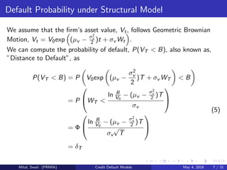
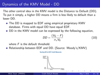
This document provides an overview of various credit default models, including: - Merton's structural model, which uses Black-Scholes option pricing theory to estimate probability of default. - Extensions to Merton's model, including the KMV model which maps "distance to default" to historical default rates. - Ratings-based models that use credit rating migration probabilities provided by rating agencies. - Multivariate factor models that model default dependence between firms using common factors like the economy. The document discusses key aspects and assumptions of these different modeling approaches.