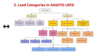
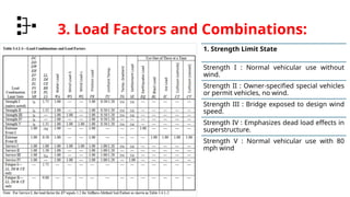
Loads &
Load Combinations to AASHTO
Presentation by
Hariyali
March 21, 2025
Flow of Presentation
1. Philosophy of LRFD
2. Load Categories in AASHTO LRFD
3. Load factors & Combinations
4. Load Calculation
Figure 1.1 Graphical Representation of LRFD
≥
1. LRFD Philosophy
• The primary goal of structural design is to
size members and components while
ensuring the structure is safe, efficient,
and cost-effective. This aligns perfectly
with the LRFD approach.
β=
𝑔𝑚𝑒𝑎𝑛
σ 𝑔
= R-DL-LL
∑η𝑖γ𝑖𝑄𝑖≤𝜙𝑅𝑛…1.3.2.1-1 (AASHTO LRFD)
= resistance factor
=nominal resistance
= load modifier
= load factor
=force effect/nominal load
LRFD (Load and Resistance Factor
Design)
ASD (Allowable/working Stress Design)
1. It applies safety factors directly to both
the loads and material Strengths. It
results in a design that balances both
factors for more efficient and
consistent safety levels.
1. The traditional method, which applies
safety factors only to the material
Strength, tends to be more
conservative and less optimized.
2. Provides a statistically optimized
safety margin.
2. Provides a fixed safety margin.
3. More efficient by optimizing safety 3. Often over-conservative, leading to
Figure 1.1 Graphical Representation f LRFD
Figure 1.2 Graphical Representation of ASD
Resistance factor𝑹𝒓=𝝓𝑹𝒏
For all other limit states: = 1.0
For the strength limit
state
∑η𝑖γ𝑖𝑄𝑖≤𝜙𝑅𝑛
∅= 0.90 (tension-controlled
reinforcement concrete section)
= 1.0 (tension-controlled prestressed
concrete sections with bonded
strands)
= 0.90 (tension-controlled prestressed
concrete sections with
unbonded strands)
(shear and torsion
reinforcement concrete section)
(shear and torsion in monolithic
prestressed concrete and CIP
prestressed )
(compression-controlled
concrete section with spiral or
ties)
= 0.90
= 0.85
= 0.75
(bearing on concrete)
= 0.75
2. Load Categories in AASHTO LRFD
3. Load Factors and Combinations:
1. Strength Limit State
Strength I : Normal vehicular use without
wind.
Strength II : Owner-specified special vehicles
or permit vehicles, no wind.
Strength III : Bridge exposed to design wind
speed.
Strength IV : Emphasizes dead load effects in
superstructure.
Strength V : Normal vehicular use with 80
mph wind
2. Extreme Event Limit States
Extreme Event I : Includes earthquake load
Extreme Event II : Accounts for ice loads, vessel
and vehicle collisions, check floods
3. Service Limit State
Service I : Under regular operational use with a 70-
mph wind load.
Service II : Unique truck loading (e.g., access roads
to ports/industrial sites).
Service III : Tension crack control in prestressed
concrete superstructures
Service IV : Manage tension specifically in
prestressed concrete columns
4. Fatigue and fracture Limit State
Fatigue I : related to infinite load-
induced fatigue life.
Fatigue II : related to finite load-
induced fatigue life.
HS20-FTG Design Truck footprint for Fatigue Design
4. Load Calculation
Dead Loads (DC and DW)
• Dead Load (DC):
• Dead loads refer to permanent, static loads from the structure itself and barriers. They are calculated using
the following steps:
• Load Determination:
• Dead Load = Material Density × Volume of the Structural Element
• Wearing Surface Dead Load (DW):
• This includes the weight of the road surface and other fixtures that are not part of the primary structural
system. Asphalt or concrete wearing surfaces are calculated similarly to structural dead loads.
Vehicular Live Loads (LL)
• AASHTO uses a standardized truckload model called HL93 for design. This represents
a typical truck weight and configurations, including axle loads and spacing.
Design for Truck
1.Design Truck HL-93
2.Design Tandem HL-93
3.Design Lane Load
HL-93
Fig. 1.3 Permit Vehicle
(Federal Highway
Fig. 1.2 Lane and Truck
Loading Combination
3.6.1.2.2-1—Characteristics of the Design Truck (AASHTO)
Fig. 1.2 Design Lane Load
(AASHTO)
HL-93TRK
HL-93TDM
Fig. 1.1 Design Tandem
(AASHTO)
Number of Design Lanes
•Standard design lane width = 12.0 ft, unless specified otherwise.
•Number of design lanes = integer part of (clear roadway width / 12.0 ft).
•If traffic lanes are narrower than 12.0 ft, use actual traffic lane width, and
number of lanes equals actual number of traffic lanes.
•For roadway widths between 20 and 24 ft, always use two design lanes, each half
of the roadway width.
Multiple Presence Factor
MPF ensures a realistic assessment of bridge loads
by considering that not all lanes are likely to
experience their full design loads simultaneously
under normal traffic conditions.
Dynamic Load Allowance
(IM)
The impact factor accounts for the dynamic
effects of vehicles moving over the bridge.
According to AASHTO:
• 1.75 for deck joints
• 1.15 for fatigue limit states
• 1.33 for all other limit states
Centrifugal Forces
(CE)
The centrifugal effect on live load shall be
taken as the product of the axle weights of
the design truck or tandem and the factor C
where,
Centrifugal forces shall be applied
horizontally at a distance 6.0 ft above the
roadway surface.
𝐶= 𝑓 𝑥
𝑣2
𝑔𝑅 ………………………..….(3.6.3-1)
• A pedestrian load of 0.075 kilo-pound
per square foot shall be applied to all
sidewalks wider than 2.0 ft and
considered simultaneously with the
vehicular design live load in the
vehicle lane.
Pedestrian Loads (PL)
Braking Loads (BR)
The braking force shall be taken as the greater of:
1. 25 percent of the axle weights of the design truck or design tandem, or
2. Five percent of the design truck plus lane load or five percent of the design tandem
plus lane load
• This braking force shall be placed in all design lanes irrespective of traffic direction.
• These forces shall be assumed to act horizontally at a distance of 6.0 ft above the
roadway
• The multiple presence factors shall apply
Vehicular Collision Force (CT)
• To protect structures from collisions, we have two options:
1.Provide Structural Resistance, or
2.Redirect/Absorb Collision Load using Barriers.
Option 1: Structural Resistance
• If we choose to make the structure resist the collision, the pier or abutment should
be designed to resist a 600 kip static force,
This force is applied:
• Horizontally in a direction ranging from 0 to 15 degrees from the edge of
pavement,
• At a height between 2 to 5 feet above ground
Option 2: Redirect or Absorb Using Barrier
• Use a 42-inch high MASH TL-5 crash-tested rigid concrete barrier.
• Place the barrier at least 3.25 feet away from the face of the pier.
Water Loads (WA)
1. Static Water Pressure,
2. Buoyancy, and
3. Stream Pressure — which includes both longitudinal and lateral
components
1. Static Water Pressure
𝑝=
1
2
𝛾 𝑊 𝐻 2
2. Buoyancy
𝑝=𝛾 𝑊 𝑥 𝑉
= Unit weight of water
= height of water above base
= Unit weight of water
= Volume of submerged part of the structure
Water Loads (WA)
𝑝=
𝐶 𝐿𝑉 2
1000
3. Stream Pressure (Flowing Water Pressure)
a) Longitudinal stream Pressure
b) Lateral Stream Pressure
𝑝=
𝐶 𝐷𝑉 2
1000
Wind loads are calculated based on wind velocity, exposure category, and the area
exposed to wind.
Calculation:
WS = Wind Pressure × Exposed Area
Wind pressure on a bridge is a function of the wind speed, air density, and the area of
the structure exposed to wind.
The general equation for wind pressure acting on a surface is given by:
Where:
= Design wind pressure (ksf)
= Design 3-second gust wind speed specified (mph); (Table 3.8.1.1.2-1)
= Pressure exposure and elevation coefficient,
G = Gust effect factor, accounting for fluctuations in wind speed over time (Table
3.8.1.2.1-1)
CD = Drag coefficient (Table 3.8.1.2.1-2)
Wind Loads (WS & WL)
𝑝 𝑧=2.56 𝑥10−6
𝑉 2 𝐾 𝑧𝐺𝐶 𝐷
Figure 3.8.1.1.2-1 Design Wind Speed , in mph (m/s)
𝒑 𝒛=𝟐.𝟓𝟔 𝒙𝟏𝟎−𝟔
𝑽 𝟐𝑲 𝒛 𝑮𝑪 𝑫
𝒑 𝒛=𝟐.𝟓𝟔 𝒙𝟏𝟎−𝟔
𝑽 𝟐𝑲 𝒛 𝑮𝑪 𝑫
Factors Affecting Wind Pressure Based on Location:
Wind Loads (WL & WS) Cont.
Ground Surface Roughness Wind
Exposure
Distance Conditions
Urban, suburban, wooded areas
(Category B)
B >1,500 ft for mean height 33 ft, or
≤
>2,600 ft or 20H for height >33 ft
Open terrain, scattered obstructions
(Category C)
C All cases where B or D do not apply
Large bodies of water, flat
unobstructed areas
(Category D)
D >5,000 ft or 20H, or
Structure is within 600 ft or 20H from
Category D surface
= 0.71
= 1.00
= 1.15
for z = 33 feet
𝒑 𝒛=𝟐.𝟓𝟔 𝒙𝟏𝟎−𝟔
𝑽 𝟐𝑲 𝒛 𝑮𝑪 𝑫
Wind Loads (WL & WS) Cont.
Wind Load on Live Load:
For typical girder and slab bridges (span 150 ft and height 33 ft)
≤ ≤
1. Transverse component : 0.10 klf transverse
2. Longitudinal component : 0.04 klf longitudinal
Vertical Wind Pressure: Vertical wind pressure x Width of deck (including parapets and
sidewalks)
• 0.020 ksf for Strength III load combination
• 0.010 ksf for Service IV load combination
Vertical wind load is considered only for Strength III ( does not include wind on live load,
WL) and Service IV load combinations.
Wind Loads (WL & WS) Cont.
Thermal Load
• There are two thermal effects which potentially induce stresses in bridges, these are :
1. Uniform Temperature:
2. Gradient Temperature:
Uniform Temperature:
1. Procedure A Temperature Ranges
………………………………………………3.12.2.3-1
Coefficient of thermal expansion (e.g., 6.5×10 6
−
/F for steel)
= Length of member
2. Procedure B Temperature Ranges
Determination of Design Temperatures:
For concrete girder bridges with concrete decks:
=To be obtained from Figure 3.12.2.2-1.
=To be obtained from Figure 3.12.2.2-2.
For steel girder bridges with concrete decks:
= To be obtained from Figure 3.12.2.2-3.
= To be obtained from Figure 3.12.2.2-4.
Temperature Gradient :
Zone T1F T2F
1 -16.2 -4.2
2 -13.8 -3.6
3 -12.3 -3.3
Decks With an Asphalt Overlay
Zone T1F T2F
1 -10.8 -2.8
2 -9.2 -2.4
3 -8.2 -2.2
4 -7.6 -1.8
Plain Concrete Decks
Positive Gradient
Thank You !
Any Questions…

Loads and Load Combinations by AASHTO.pptx

  • 1.
    Loads & Load Combinationsto AASHTO Presentation by Hariyali March 21, 2025
  • 2.
    Flow of Presentation 1.Philosophy of LRFD 2. Load Categories in AASHTO LRFD 3. Load factors & Combinations 4. Load Calculation
  • 3.
    Figure 1.1 GraphicalRepresentation of LRFD ≥ 1. LRFD Philosophy • The primary goal of structural design is to size members and components while ensuring the structure is safe, efficient, and cost-effective. This aligns perfectly with the LRFD approach. β= 𝑔𝑚𝑒𝑎𝑛 σ 𝑔 = R-DL-LL ∑η𝑖γ𝑖𝑄𝑖≤𝜙𝑅𝑛…1.3.2.1-1 (AASHTO LRFD) = resistance factor =nominal resistance = load modifier = load factor =force effect/nominal load
  • 4.
    LRFD (Load andResistance Factor Design) ASD (Allowable/working Stress Design) 1. It applies safety factors directly to both the loads and material Strengths. It results in a design that balances both factors for more efficient and consistent safety levels. 1. The traditional method, which applies safety factors only to the material Strength, tends to be more conservative and less optimized. 2. Provides a statistically optimized safety margin. 2. Provides a fixed safety margin. 3. More efficient by optimizing safety 3. Often over-conservative, leading to Figure 1.1 Graphical Representation f LRFD Figure 1.2 Graphical Representation of ASD
  • 5.
    Resistance factor𝑹𝒓=𝝓𝑹𝒏 For allother limit states: = 1.0 For the strength limit state ∑η𝑖γ𝑖𝑄𝑖≤𝜙𝑅𝑛 ∅= 0.90 (tension-controlled reinforcement concrete section) = 1.0 (tension-controlled prestressed concrete sections with bonded strands) = 0.90 (tension-controlled prestressed concrete sections with unbonded strands) (shear and torsion reinforcement concrete section) (shear and torsion in monolithic prestressed concrete and CIP prestressed ) (compression-controlled concrete section with spiral or ties) = 0.90 = 0.85 = 0.75 (bearing on concrete) = 0.75
  • 6.
    2. Load Categoriesin AASHTO LRFD
  • 7.
    3. Load Factorsand Combinations: 1. Strength Limit State Strength I : Normal vehicular use without wind. Strength II : Owner-specified special vehicles or permit vehicles, no wind. Strength III : Bridge exposed to design wind speed. Strength IV : Emphasizes dead load effects in superstructure. Strength V : Normal vehicular use with 80 mph wind
  • 9.
    2. Extreme EventLimit States Extreme Event I : Includes earthquake load Extreme Event II : Accounts for ice loads, vessel and vehicle collisions, check floods 3. Service Limit State Service I : Under regular operational use with a 70- mph wind load. Service II : Unique truck loading (e.g., access roads to ports/industrial sites). Service III : Tension crack control in prestressed concrete superstructures Service IV : Manage tension specifically in prestressed concrete columns
  • 10.
    4. Fatigue andfracture Limit State Fatigue I : related to infinite load- induced fatigue life. Fatigue II : related to finite load- induced fatigue life. HS20-FTG Design Truck footprint for Fatigue Design
  • 11.
    4. Load Calculation DeadLoads (DC and DW) • Dead Load (DC): • Dead loads refer to permanent, static loads from the structure itself and barriers. They are calculated using the following steps: • Load Determination: • Dead Load = Material Density × Volume of the Structural Element • Wearing Surface Dead Load (DW): • This includes the weight of the road surface and other fixtures that are not part of the primary structural system. Asphalt or concrete wearing surfaces are calculated similarly to structural dead loads.
  • 12.
    Vehicular Live Loads(LL) • AASHTO uses a standardized truckload model called HL93 for design. This represents a typical truck weight and configurations, including axle loads and spacing. Design for Truck 1.Design Truck HL-93 2.Design Tandem HL-93 3.Design Lane Load HL-93 Fig. 1.3 Permit Vehicle (Federal Highway Fig. 1.2 Lane and Truck Loading Combination 3.6.1.2.2-1—Characteristics of the Design Truck (AASHTO) Fig. 1.2 Design Lane Load (AASHTO) HL-93TRK HL-93TDM Fig. 1.1 Design Tandem (AASHTO)
  • 13.
    Number of DesignLanes •Standard design lane width = 12.0 ft, unless specified otherwise. •Number of design lanes = integer part of (clear roadway width / 12.0 ft). •If traffic lanes are narrower than 12.0 ft, use actual traffic lane width, and number of lanes equals actual number of traffic lanes. •For roadway widths between 20 and 24 ft, always use two design lanes, each half of the roadway width. Multiple Presence Factor MPF ensures a realistic assessment of bridge loads by considering that not all lanes are likely to experience their full design loads simultaneously under normal traffic conditions.
  • 14.
    Dynamic Load Allowance (IM) Theimpact factor accounts for the dynamic effects of vehicles moving over the bridge. According to AASHTO: • 1.75 for deck joints • 1.15 for fatigue limit states • 1.33 for all other limit states Centrifugal Forces (CE) The centrifugal effect on live load shall be taken as the product of the axle weights of the design truck or tandem and the factor C where, Centrifugal forces shall be applied horizontally at a distance 6.0 ft above the roadway surface. 𝐶= 𝑓 𝑥 𝑣2 𝑔𝑅 ………………………..….(3.6.3-1)
  • 15.
    • A pedestrianload of 0.075 kilo-pound per square foot shall be applied to all sidewalks wider than 2.0 ft and considered simultaneously with the vehicular design live load in the vehicle lane. Pedestrian Loads (PL) Braking Loads (BR) The braking force shall be taken as the greater of: 1. 25 percent of the axle weights of the design truck or design tandem, or 2. Five percent of the design truck plus lane load or five percent of the design tandem plus lane load • This braking force shall be placed in all design lanes irrespective of traffic direction. • These forces shall be assumed to act horizontally at a distance of 6.0 ft above the roadway • The multiple presence factors shall apply
  • 17.
    Vehicular Collision Force(CT) • To protect structures from collisions, we have two options: 1.Provide Structural Resistance, or 2.Redirect/Absorb Collision Load using Barriers. Option 1: Structural Resistance • If we choose to make the structure resist the collision, the pier or abutment should be designed to resist a 600 kip static force, This force is applied: • Horizontally in a direction ranging from 0 to 15 degrees from the edge of pavement, • At a height between 2 to 5 feet above ground Option 2: Redirect or Absorb Using Barrier • Use a 42-inch high MASH TL-5 crash-tested rigid concrete barrier. • Place the barrier at least 3.25 feet away from the face of the pier.
  • 18.
    Water Loads (WA) 1.Static Water Pressure, 2. Buoyancy, and 3. Stream Pressure — which includes both longitudinal and lateral components 1. Static Water Pressure 𝑝= 1 2 𝛾 𝑊 𝐻 2 2. Buoyancy 𝑝=𝛾 𝑊 𝑥 𝑉 = Unit weight of water = height of water above base = Unit weight of water = Volume of submerged part of the structure
  • 19.
    Water Loads (WA) 𝑝= 𝐶𝐿𝑉 2 1000 3. Stream Pressure (Flowing Water Pressure) a) Longitudinal stream Pressure b) Lateral Stream Pressure 𝑝= 𝐶 𝐷𝑉 2 1000
  • 20.
    Wind loads arecalculated based on wind velocity, exposure category, and the area exposed to wind. Calculation: WS = Wind Pressure × Exposed Area Wind pressure on a bridge is a function of the wind speed, air density, and the area of the structure exposed to wind. The general equation for wind pressure acting on a surface is given by: Where: = Design wind pressure (ksf) = Design 3-second gust wind speed specified (mph); (Table 3.8.1.1.2-1) = Pressure exposure and elevation coefficient, G = Gust effect factor, accounting for fluctuations in wind speed over time (Table 3.8.1.2.1-1) CD = Drag coefficient (Table 3.8.1.2.1-2) Wind Loads (WS & WL) 𝑝 𝑧=2.56 𝑥10−6 𝑉 2 𝐾 𝑧𝐺𝐶 𝐷
  • 21.
    Figure 3.8.1.1.2-1 DesignWind Speed , in mph (m/s) 𝒑 𝒛=𝟐.𝟓𝟔 𝒙𝟏𝟎−𝟔 𝑽 𝟐𝑲 𝒛 𝑮𝑪 𝑫
  • 22.
    𝒑 𝒛=𝟐.𝟓𝟔 𝒙𝟏𝟎−𝟔 𝑽𝟐𝑲 𝒛 𝑮𝑪 𝑫 Factors Affecting Wind Pressure Based on Location: Wind Loads (WL & WS) Cont. Ground Surface Roughness Wind Exposure Distance Conditions Urban, suburban, wooded areas (Category B) B >1,500 ft for mean height 33 ft, or ≤ >2,600 ft or 20H for height >33 ft Open terrain, scattered obstructions (Category C) C All cases where B or D do not apply Large bodies of water, flat unobstructed areas (Category D) D >5,000 ft or 20H, or Structure is within 600 ft or 20H from Category D surface = 0.71 = 1.00 = 1.15 for z = 33 feet
  • 23.
    𝒑 𝒛=𝟐.𝟓𝟔 𝒙𝟏𝟎−𝟔 𝑽𝟐𝑲 𝒛 𝑮𝑪 𝑫 Wind Loads (WL & WS) Cont.
  • 24.
    Wind Load onLive Load: For typical girder and slab bridges (span 150 ft and height 33 ft) ≤ ≤ 1. Transverse component : 0.10 klf transverse 2. Longitudinal component : 0.04 klf longitudinal Vertical Wind Pressure: Vertical wind pressure x Width of deck (including parapets and sidewalks) • 0.020 ksf for Strength III load combination • 0.010 ksf for Service IV load combination Vertical wind load is considered only for Strength III ( does not include wind on live load, WL) and Service IV load combinations. Wind Loads (WL & WS) Cont.
  • 25.
    Thermal Load • Thereare two thermal effects which potentially induce stresses in bridges, these are : 1. Uniform Temperature: 2. Gradient Temperature: Uniform Temperature: 1. Procedure A Temperature Ranges ………………………………………………3.12.2.3-1 Coefficient of thermal expansion (e.g., 6.5×10 6 − /F for steel) = Length of member
  • 26.
    2. Procedure BTemperature Ranges Determination of Design Temperatures: For concrete girder bridges with concrete decks: =To be obtained from Figure 3.12.2.2-1. =To be obtained from Figure 3.12.2.2-2. For steel girder bridges with concrete decks: = To be obtained from Figure 3.12.2.2-3. = To be obtained from Figure 3.12.2.2-4.
  • 27.
    Temperature Gradient : ZoneT1F T2F 1 -16.2 -4.2 2 -13.8 -3.6 3 -12.3 -3.3 Decks With an Asphalt Overlay Zone T1F T2F 1 -10.8 -2.8 2 -9.2 -2.4 3 -8.2 -2.2 4 -7.6 -1.8 Plain Concrete Decks Positive Gradient
  • 28.
    Thank You ! AnyQuestions…

Editor's Notes

  • #1 Hii, Good afternoon everyone. Today I’ll be presenting on Loads and Loads combinations as per AASHTO. This is beginner's presentation for those transitioning into the USA market. Those already familiar with AASHTO can treat this as a refresher.
  • #2 ASHTO LRFD Bridge Design Specifications consist of 15 sections. Today, we will focus on the 1st section which is Introduction and the 3rd section which is Loads and Load Factors. The code is based on Limit States Design same as Indian code.
  • #3 Let's start with the LRFD philosophy 😊The primary goal of structural design is to size members and components while ensuring that the structure is safe, efficient, and cost-effective. LRFD approach aligns perfectly with this . LRFD ensures safety using probability-based reliability. The first graph on top left side is The bell curve which illustrates the probability distributions of applied loads and structural resistance. In graph, the mean applied load, Q mean represents loads acting on bridge and mean Resistance, Rmean is the strength of bridge. However, due to variations in loads and resistance, we apply a load factor Gama i to account for uncertainties in load which increase the design load and Since materials and construction can have variations as well, we apply a resistance factor phi, to reduce the nominal resistance, Rn. The gap between these two values represents the safety margin which ensures the structure remains reliable and has very low probability of failure that is shown in figure 1.1 Now, let’s see how we quantify this safety margin using the Reliability Index (β). β is the ratio of the mean safety margin to its standard deviation. The Reliability Index (β) quantifies structural risk statistically. A higher β means a safer structure with a lower probability of failure. In AASHTO LRFD, β values are typically between 3.5 to 4.0, ensuring a failure probability is between 1 in 10,000 to 1 in 1,000,000. This approach which we used in LRFD helps optimizing design while maintaining high safety standards. the fundamental equation given for structure design is resistance offered should be greater than or equal to summation of load effects.
  • #4 Now the difference between Load resistance factor design and working stress design is mainly given by these 3 points.
  • #5 There are two key factors load factors (γ) and resistance factors, load factors depends on the type of loads and we will look at their values once we figure out what kinds of loads we're dealing in bridge design. Coming to Resistance factors (Φ) which we use to reduce material strength to ensure safety and that is given by the graph here. This graph shows change in resistance factor based on strain (ε) in reinforced and prestressed concrete section. Left Side zone is for compression controlled concrete section, which has lower resistance factor Φ = 0.75, Middle transition zone is for sections which lies between compression controlled section and tension controlled section and Φ values shall be obtained by linear interpolation from given formulas based on section is prestressed of non-prestressed. Right Side zone is for tension-controlled sections and phi is 0.9 for non prestressed and 1.0 for prestressed tension-controlled sections. In IRC: The material factor for concrete is 1.5, so 1/factor or safety, 1.5 is 0.66, and for steel, it is 1.15, meaning 1/factor of safety 1.15 is 0.87 , In both codes that can be relatable as Concrete needs a higher safety factor (lower Φ) because it fails suddenly. Steel has a lower safety factor (higher Φ) because it is ductile and allows deformation before failure.
  • #6 Moving forward with the types of loads. The loads acting on a bridge are classified into Permanent Loads and Transient Loads. Permanent loads are the loads such as self-weight, superimposed dead loads and material creep & shrinkage which remain throughout the bridge’s lifespan. Transient loads are the loads which are temporary or vary over time, including traffic loads, environmental effects, and loads due to construction activities. Traffic loads are further divided into primary vertical loads and secondary horizontal loads, where vertical loads include normal, abnormal and exceptional loading. Normal loads that is the regular traffic like cars and trucks present on roads, abnormal loads that account for rare occurrences of vehicles like fire tenders or military vehicles, and exceptional loads are like permit trucks carrying gas turbines, windmill components.. Etc. Secondary horizontal loads are due to the primary vertical loads when they undergo actions like braking, acceleration, turning or colliding with bridge component. Bridge also faces challenges from natural forces like wind, earthquake, heating or cooling, Ice and snow and water current depending upon season and location.
  • #7 It’s important to remember that these loads don’t act individually, In reality multiple loads often act together. Depending on their probability and intensity, We combine them systematically what we call as Load Combinations. In Table 3.4.1-1, we have the Load Combinations and Load Factors. There is strength, extreme event, service and fatigue load combinations. Strength limit state is to ensure Strength and stability, both locally and globally. There are five load combinations for strength. Strength I and strength II are without wind load. Strength I is for normal everyday traffic. Strength II addresses special heavy vehicles like emergency or permit trucks. Strength III combines design wind speed with dead load for locations where wind can be significant. Strength IV focuses on dead loads and does not include live load and wind load. This combination shall not be used for foundation design as it has minimum vertical load and minimum lateral load, which will not give an adequate foundation design. Strength V accounts for normal traffic combined with 80 mph wind. GO TO NEXT SLIDE
  • #8 Tables 3.4.1-2, and 3 provide the minimum and maximum load factors for permanent loads. Depending on the design situation – if a load contributes unfavourably to the situation we us maximum load factor. And If the load contributes favourably, we use the minimum load factor. In complicated situations it is wise to form two combinations one using maximum and one using minimum load factor. For design we can use the envelope and decide the governing load effects.
  • #9 Then There are Extreme Event Load Combinations to account for preventing collapse and not preventing damage. Extreme Event one is related to Seismic event. Extreme Event two covers events like ice loads, collisions from vessels and vehicles. We assume no two extreme events occur simultaneously. For these cases, a reduced live load is used. Serviceability load combinations are to check for users' comfort, we check deflection, cracking and vibration. Service one is used for normal, everyday bridge use, and it includes 70 mph wind, with all loads taken at unfactored values. This combination checks deflection control in buried structure. It also ensures crack width control in reinforced concrete and checks transverse tension in segmental concrete girders. Service two focuses on preventing yielding in steel structures and slip in slip-critical connections under vehicular live loads. Load factor for live loads in service 2 is 1.3 and can be adjusted if the bridge serves special areas like port or industrial access roads. Service III deals with longitudinal tension in prestressed concrete superstructures, with the main goal of controlling cracks and Service IV is specific to prestressed concrete columns, focusing on controlling tension and cracks.
  • #10 Fatigue limit state is to limit crack growth under cyclic loading to prevent fracture. Fatigue load combination is applied to a single design truck. In Fatigue one load combination stress range we check against infinite fatigue life. And in Fatigue two load combination is used when we design structure component to withstand a specific number of load cycles. For isotropic decks in fatigue load one design truck, with a constant spacing of 30.0 ft between the 32.0-kilo pounds axles is consider while for orthotropic decks we use truck given in figure 3.6.1.4.1.1-1.
  • #11 Now Load calculation: Dead load is weight of all the structure components along with wearing coat and utilities and railings. The calculation is simple, volume multiply with unit weight of material and unit weight of different materials are given in Table 3.5.1-1.
  • #12 Design vehicular HL-93 is used to represent normal traffic for bridge design. HL-93 is combination of these three loads. Design Truck HL-93, Design tandem HL-93 and Design Lane Load. The total gross weight of Design truck is 72 kilo-pounds. And it consists of a single axle load of 8 kilo-pound, and Two axles of 64 kilo-pounds each carrying a load of 32 kilo-pounds. The spacing between 8 kilo-pounds axle and the first 32 kilo pounds axle is 14 feet, while axle spacing between two 32 kilo-pounds axles can be varied between 14 feet to 30 feet. Design Tandem consists of a pair of 25 kilo pounds axles spaced at 4 feet apart. The transverse spacing of wheels is 6 feet in design truck and tandem both. The design lane load is a Uniform load of 640 pound per linear foot that spread out over a 10 feet width. Each design lane we analyze is assumed to carry either the truck combined with the lane load or tandem combined with the lane load.
  • #13 Now number of design lanes…………………….The idealized width of a design lane is 12 feet. Number of design lane is the whole number from carriage width divided by lane width. The Multiple presence factor is a reduction factor used for acknowledging that the probability of multiple vehicles being present at the same time at same location in two adjacent lanes is lower than one. The applicable values for Multiple presence factor are provided in Table 3.6.1.2-1. Now for Single traffic lane alone the Multiple presence factor is greater than one, the reason behind this is when we are considering single lane and single vehicle, this single vehicle can be heavier than two lighter vehicles and it also possess the same probability of occurrence.
  • #14 Dynamic load allowance which is Impact factor is applied to account for the dynamic effects and These dynamic effects mainly come from two sources: the hammering effect due to surface roughness like joints and potholes, and the bridge’s vibration response to moving vehicles. Impact factor is applied only for trucks and tandems, not for lane loading and pedestrian loading. For deck joints impact factor is 1.75 and all other components it is 1.33. Moving to centrifugal force When vehicles move on curved bridges, centrifugal force creates a radial force and an overturning effect. This force is calculated using a factor 'C', which depends on the vehicle speed and curve radius. In formula f is 1 for fatigue and 4/3=1.33 for all other load combinations and g is gravitational acceleration: 32.2 (ft/s2). Centrifugal force is applied horizontally at 6 feet above the roadway.
  • #15 Now let’s talk about Braking Force (BR) —It is a horizontal force we apply to simulate the effect of vehicles braking on a bridge. The braking force should be taken as the greater of two values: (one) 25% of the axle weights of the design truck or tandem or (two) 5% of the combined weight of the design truck plus lane load, or design tandem plus lane load. Braking force is applied in all design lanes in the same direction that are carrying traffic considering the possibility of one-directional traffic in future and it needs to apply at 6 feet above road surface. Moving forward to pedestrian live load For bridges with both vehicular and pedestrian load and with a more than 2-feet-wide sidewalk, a pedestrian load of 75 pounds per square foot should be applied to the sidewalk in design. When vehicles can drive onto the sidewalk, or when the sidewalk is expected to be removed within the bridge design life, vehicular live load should be applied in that portion of the bridge. In such case vehicular live load should be applied at 1 foot from the deck edge for design of the overhang and at 2 feet from the deck edge for design of all other bridge elements.
  • #16 Ohh, so that is exactly why our bridges are actually designed to take that hit!😃 We account this Vehicular collision forces while designing piers and abutments that are located within the roadway's clear zone. We need to protect structures from collisions and we have two options: Either we make the structure robust enough to sustain accidental hits from vehicles, or by Redirecting vehicle or by Absorbing Collision Load using Barriers. When we decide to design a pier or abutment to resist a vehicle collision,…. -this is like saying, "Let's plan for a huge vehicle hit and see if the structure can handle it. In that case we consider a static force of 600 kips (kilo pounds ) acting horizontally at any angle between 0 and 15 degrees from the edge of the pavement this will to simulate a straight or slightly angled vehicle hit. The height of impact should be taken between 2 to 5 feet above the ground, depending on what creates the maximum shear or moment in the pier or its connections to the foundation or cap. If we choose option 2 we should provide rigid barrier with height of at least 42 inches at 3.25 feet away from the face of the pier component that can sustain crash test of MASH Test Level-5.
  • #18 let's talk about Water Loads (WA), which are important when a bridge is over river or waterbody, So in water loads, we consider hydrostatic and hydrodynamic pressure— In hydrostatic pressure first is from still water which is given by the area of the triangle which acts at a distance 1/3rd from base and that increases with depth. second is Buoyancy force, that is simply an uplift force equal to the weight of the volume of water displaced by the submerged part. Density of water is lower than density of concrete, thus buoyancy would not be a problem for solid structures. But for hollow structures like underground storage tanks, cellular abutments, or hollow piers, it should be investigated..
  • #19 In hydrodynamic force. First is the longitudinal stream pressure acts directly along the water flow and this depends on how fast water is flowing and the shape of the pier. Here in table Semicircular pier face less force as drag coefficient is 0.7 and square ended pier face higher force with drag coefficient of 1.4. The second is lateral stream pressure, which we calculate by this formula and by considering the fact that water can hit the pier at an angle. The lateral drag coefficient for different angles is given in Table 3.7.2.1.
  • #20 When wind acts on a bridge, it creates a horizontal pressure on the bridge. This pressure is uniformly distributed over the exposed surface area, including the structure and live load. The total wind load is simply the wind pressure multiplied by the exposed area. Wind pressure is given by this formula 2.56 into 10 power minus 6 into square of design 3-second gust wind speed as per table given into the coefficient for pressure exposure and elevation multiply by gust factor and drag coefficient.
  • #21 In this formula, design wind speed V, used for calculating wind loads, depends on the geographic location of a bridge, as it varies with regional weather conditions and topography. From the table we can see that For Load Combination Strength III, the wind speed should be taken from the standard wind speed map provided in Figure 3.8.1.1.2-1 of AASHTO code. For Strength V and Service I wind speeds are 80 and 70 mph respectively and Service IV load combination it is 0.75 of what we get from the map.
  • #22 In this formula of wind pressure, Kz is the exposure factor. Now when wind is running toward bridge —First question to know "What kind of land is wind running over?" (That’s terrain exposure and given by ground Surface Roughness). Then, second question is "For how long is this land type continuing before it hits bridge?" (That's used to decide Wind Exposure Category). Based on these two answers, we would come to know how strong and turbulent the wind is when it finally hits the bridge. Wind Exposure Category B is selected when a bridge is located in an urban or suburban area, meaning Ground Surface Roughness is Category B. This applies when, within a radius of 1,500 feet or more around the bridge, the average height of surrounding buildings is 33 feet or less. Exposure B continues if, for a maximum of either a radial distance of 2,600 feet or 20 times the height of the bridge, the mean height of structures is more than 33 feet. . Wind Exposure Category D is used when a bridge is located in a completely open and flat area. For category D when a bridge height is 33 feet, The Coefficient of Exposure is 1.15– which is more than the category B which is 0.71 & more than category C which is 1.0– and that makes sense as Category D applies to open terrain with no obstructions and therefore wind density is higher. Wind Exposure Category C is selected when a bridge is located in open terrain with scattered obstructions and that is when it lies between category B and category D.
  • #23 Gust is a sudden increase in wind speed that creates short-term but significant forces on a bridge and must be considered in design using the Gust effect factor table. The Drag Coefficient is a dimensionless factor that represents wind force based on the shape of the structure; values are provided in the Drag coefficient table. Using this wind pressure, various angles of attack for wind direction should be investigated to determine which angle produces the worst case response in the bridge substructure. For resolving the wind acting at an angle respect to perpendicular to the bridge’s longitudinal axis, Skew coefficient table is given for various skew angles for superstructure and substructure. Now wind load on superstructure can be calculated by multiplying wind pressure (Pz), girder depth and the skew coefficient in table. we will get both the components of the wind loads and longitudinal component shall be applied as line loads at the mid-depth of the girders along the longitudinal axis of the superstructure. While transverse wind load we apply in transverse direction as point load by creating a rigid link from bearing to mid depth of girder. And wind load on substructure can be calculated by The wind pressure multiplied by skew coefficient and exposed substructure area as seen in end elevation shall be the Longitudinal wind force and the wind pressure multiplied by skew coefficient and exposed substructure area as seen in front elevation shall give the transverse wind force. Both components of superstructure and substructure wind force shall be applied simultaneously. For typical girder and slab bridges with span up to 150 ft and height less than 33 ft, the angle of attack can be assumed as zero. Longitudinal force can be assumed as 25% of full wind load acting transversely.
  • #24 When wind blows across a bridge, it doesn’t just affect the bridge structure but also the vehicles (live load) on it . For typical girder and slab bridges with span up to 150 ft and height less than 33 ft, the angle of attack of wind on vehicles can be assumed as zero. For such bridges transverse wind load is 0.1 kilo pound per linear foot and Longitudinal force can be assumed as 25% of transverse wind load. For other bridges Longitudinal and transverse forces are given in the table 3.8.1.3.-1 Now strong winds can create an upward lifting force, Known as vertical wind loads, This force acts across the entire deck width, including sidewalks and parapets. It is applied at the windward quarter-point of the deck width. We use vertical wind load for only two load combinations Strength III and Service IV and that is too only when wind is blowing perpendicular to the bridge.
  • #25 Thermal loads are critical in bridge design because temperature changes can cause significant expansion and contraction. Uniform temperature refers to the overall temperature change that affects the entire bridge structure, causing it to expand when heated and contract when cooled. These movements due to expansion and contraction causes axial force and moments if restrain. AASHTO provides two methods to calculate thermal movements due to uniform temperature change— Procedure A and Procedure B. Procedure A is used for all bridge types including timber, aluminium and concrete deck bridges with concrete girder or steel girder. Formula to calculate deformation is delta L = alfa L delta T is used For method A Table 3.12.2.1-1, gives maximum and minimum design temperatures based on material (Steel, Concrete, Wood) and climate (Moderate, Cold) to calculate difference in temperature.
  • #26 In Procedure B to know the maximum and minimum design temperature we use maps based on location and the type of superstructure. To calculate change in length we use the same linear expansion formula.
  • #27 Temperature gradient refers to the change in temperature through the depth of the superstructure due to environmental exposure. The top deck surface, being directly exposed to the solar radiation and the surrounding temperature, becomes hotter more than the bottom surface, as it remains relatively sheltered. These heating and cooling differentials create Temperature gradient, which results in internal stresses and deformation. Temperature gradients are of two kinds: Positive Gradient and Negative Gradient. Positive Gradient is when is when the top surface is hotter than the bottom surface For example during the day and Negative Gradient when the top surface is colder than the bottom surface like during the night. Figure 3.12.3-2 (three twelve three dash two) provides a basis for temperature variation within bridge sections. Value of T1 and T2 are depends on temperature zones. The United States has four temperature zones (Figure 3.12.3-1). Temperature values (T₁ & T₂) for the four zones are provided in Table 3.12.3-1. that is for positive gradient and for the negative gradient table needs to multiply with -0.3 and -0.2 for plain concrete deck and decks with asphalt overlay respectively. Temperature T3 shall be taken as 0 (zero degrees Fahrenheit) unless and until specify and it shall not exceed 5 . Dimension A represents a reference depth within the superstructure. For Concrete Superstructures If the total depth of the superstructure is 16 inches or more → A is 12 inches. If the depth is less than 16 inches → A is 4 inches less than the actual depth that is means if a concrete girder is 14 inches deep, A = 14 - 4 = 10 inches. For Steel Superstructures: A = 12 inches while t = total depth of the concrete deck.