This document presents a method for liver segmentation using a 2D U-Net model. The method first preprocesses CT scan images using techniques like windowing, masking, normalization, and morphological operations. It then trains a 2D U-Net model on slices containing liver regions only, in order to focus modeling on liver segmentation. To improve inference performance on full volumes which may contain non-liver slices, the method uses histogram analysis to roughly select a range of slices likely to contain liver, such as the central 40% of slices. Evaluation shows this rough selection approach improves segmentation accuracy compared to applying the model to full volumes directly.

1. LIVER SEGMENTATION WITH 2D UNET
1
Hsin-Han Tsai (蔡欣翰),1
Chiou-Shann Fuh (傅楸善)
1
Department of Computer Science and Information Engineering,
National Taiwan University, Taiwan
E-mail: d08922013@csie.ntu.edu.tw
fuh@csie.ntu.edu.tw
ABSTRACT
We proposed an idea to choose the Region Of Interest
(ROI) so that to improve the performance in inference.
In this paper, we focus on liver segmentation. It is easy
to train a liver segmentation model by using images
with liver. But it is hard to train a liver segmentation
model by using whole volume data with or without liver.
Our idea is to train a model with liver images only, and
use some computer vision method to roughly choose a
region of slices (about 40% of whole abdominal volume)
and then apply to the model. It can improve the
inference performance since the most error comes from
those data without liver.
Keywords: Liver Segmentation, UNet, Deep Learning.
1. INTRODUCTION
The liver is an organ located in the upper right part of
the abdomen. It is beneath the diaphragm and on top of
the stomach, right kidney, and intestines. The liver has
many functions. The liver's main job is to filter the blood
coming from the digestive tract, before passing it to the rest
of the body. The liver also detoxifies chemicals and
metabolizes drugs. There are some types of liver disease
include hepatitis, cirrhosis, liver cancer, and so on. The
most common type of liver cancer, hepatocellular
carcinoma, almost always occurs after cirrhosis is present.
Computer-Aided Diagnosis (CAD) has been defined as
a diagnosis made by a radiologist who uses the output
of a computer analysis of the images when making his
or her interpretation. Medical image segmentation is an
important part of CAD. However, to do a precise
segmentation is challenging due to the following
reasons: (1) The organ or tissue might be irregular shape
or shattered. (2) The imaging method is based on X-ray,
so many partitions might be cumulated. (3) Affected by
noise and artifacts. By using traditional computer vision
method, it is hard to get a good enough performance.
But nowadays, deep learning was applied to medical
image area frequently. Based on the success of deep
learning, many powerful 3D model was proposed. U-
Net was seen as the key model of segmentation task.
Liver is a large organ in human abdomen. But the shape
of the liver is irregular, even shattered in different slices.
Suppose we train a 2D model for liver segmentation, the
challenge is that some circle regions might be predicted
as liver if we do not consider the 3D information. As in
Figure 1 represents, the upper row shows that there is no
liver label in this slice, but the model predicts false
regions. And the lower row shows that if the slice
contains the liver, then the predicted segmentation
would be great.
Figure 1. Left: The preprocessed slice. Middle: The
label mask. Right: The predicted liver region relative to
the preprocessed slice. Upper row: Slice 91. Lower row:
Slice 196.
In this paper, we have introduced the methods including
data preprocessing, 2D U-Net, and roughly liver
choosing in Section 3. We showed the experiment and
results in Section 4. Finally, we gave a discussion and
conclusion in Sections 5 and 6, respectively.
2. RELATED WORKS

2. Liver segmentation task has been researched for a long
time. There were many challenges from many
conferences in the world. The famous one, MICCAI
2017 challenge [1], encourages researchers to develop
automatic segmentation algorithms to segment liver
lesions in contrast-enhanced abdominal CT scans. There
are several state-of-the-art algorithms from worldwide
researchers. The algorithms can be categorized into
several classes, deep learning 3D based [2, 3, 4, 5], deep
learning 2D based [6, 7, 8], statistical based [9, 10],
computer vision based [11]. In general, deep learning
3D based method performs better. But the trade of is
that the computations is much higher than deep learning
2D based method. For us, we still want to apply deep
learning 2D based method and combine with statistical
or computer vision methods to keep training fast and get
similar performance to deep learning 3D based method.
3. METHOD
3.1. Data Preprocessing
Computed Tomography (CT) is often used to refer to X-
ray because of the similar imaging principle. The unit in
the CT image is called Hounsfield Unit (HU) or CT
number. Hounsfield unit scale is a linear transformation
of the linear attenuation coefficients of water and air.
The HU value of liver is around 60, so it gives us a clue
for image preprocessing.
3.1.1. Windowing
Windowing is a common preprocessing method in CT
images. The effect of windowing is contrast
enhancement. The brightness of the image is adjusted by
the Window Level (WL). The contrast is adjusted by the
Window Width (WW). The window level is the
midpoint of the HU values range displayed. The
window width is the range of CT numbers that an image
contains. According to biochemistry knowledge, the HU
value of the liver is around 60. For our experiments, we
chose WL = 90 and WW = 220 to include the liver.
After image windowing, the HU values lower than -20
will be set to -20 and the HU values higher than 200
will be set to 200. The example before and after image
windowing is shown in Figure 2.
(a) Without windowing (b) Windowing
Figure 2. Before and after the image windowing. (a)
Original CT image. (b) Image windowing with WL = 90
and WW = 220.
3.1.2 Masking
To discard some image values which are higher than the
window range. Since they displayed other organs or
tissues. For our experiment, we set the CT numbers over
200 as -20. Figure 3 shows the result before and after
masking.
(a) Before masking (b) After masking
Figure 3. Remove the pixels whose CT number exceeds
200. (a) Image after windowing but before masking. (b)
Masking result of image (a).
3.1.3 Normalization
The minimum maximum normalization has been chosen.
The formula is described as follows
3.1.4 Opening
Opening is an important operator from mathematical
morphology. In simple, an opening operator is defined
as an erosion followed by a dilation using the same
structuring element. The effect of an opening operator is
to preserve foreground regions that have a similar shape
to the structure element. Figure 4 shows the image
before and after an opening operator with a 3*3
structuring element.
(a) Before opening (b) After opening
Figure 4. To show the effect of o an opening operator. (a)
Image in Figure 3(b). (b) Image (a) after opening
operation. As we can see the bed is removed.
3.1.5 Closing
Closing is an operator defined as a dilation followed by
an erosion using the same structuring element. It is a
dual operator of opening. The effect of closing is to
preserve background regions that have a similar shape

3. to the structuring element. Figure 5 shows the effect of a
closing operation (numpy.ones((3,3))).
(a) Before closing (b) After closing
Figure 5. Closing operator can remove some small holes
because of dilation first then erosion. (a) Before the
closing operation. (b) Effect of closing that some small
holes are removed.
3.2. 2D U-Net
U-Net based models are usually applied to segmentation
tasks. The reason is that it is able to localize and
distinguish borders is by doing classification on every
pixel. The model architecture is described in Figure 6.
And the details of each operation are described as below.
3.2.1 Conv2D
3.2.2 MaxPooling2D
3.2.3 UpSampling (Conv2DTranspose)
3.2.4 Concatenate
3.2.5 Model Architecture

4. Figure 6. 2D U-Net architecture. All Conv2D operators
apply 3*3 filters, strides = 1, ReLU activations, and
same padding settings.
3.3. Roughly Liver Choosing
To improve the poor performance of segmenting liver
from whole abdomen CT scan, we propose a simple
method to choose a range of slices that contain the liver.
We described it in following steps.
Step 1. Evaluate the histogram for each slice. See
Figure
7.
(a) Left: Original image in slice 42. Middle: Label
mask of the liver. Right: Histogram of the original
image.
(b) Left: Original image in slice 51. Middle: Label
mask of the liver. Right: Histogram of the original
image.
(c) Left: Original image in slice 61. Middle: Label
mask of the liver. Right: Histogram of the original
image.
Figure 7. Visualization of Step 1.
Step 2. Find the greatest number of pixels in intensity
range from -20 to 200. We suppose that the summit
represents for the liver. See Figure 8.
Figure 8. The highest place between CT numbers -20 to
200 represents the liver area. The larger area is, the
higher the peak is.
Step 3. Find the maximum liver area by finding out the
maximum in all peaks from different slices. Figure 8
actually shows the highest peak among all slices. That
means we now derive the slice which has the largest
area of the liver.
Step 4. Fix the slice we found from previous steps.
Create a range whose midpoint is the slice and range
length is 40% of the total number of slices. See Figure 9.
Figure 9. Visualization of Step 4.
From Steps 1 to 4, we derive a roughly parts that
included the liver. This may improve the accuracy in the
liver segmentation.
3.4. Workflow

5. The training work flow and inference work flow are
described in Figures 10 and 11, respectively.
Figure 10. Training work flow.
Figure 11. Inference work flow.
4. EXPERIMENTS
We had done all the experiments on the cluster with
l CPU: Intel Xeon E5-2650 2.20GHz
l Memory: 520 GB
l GPU: NVIDIA TITAN V 12GB.
And we use Keras version 2.2.4, Python version 3.6 to
do the research. We applied Dice score and Dice loss to
be the measurement of the accuracy and the loss,
respectively. We use Adam optimizer with initial
learning rate 0.001. The learning rate would be divided
by 10 if the validation loss did not improve in 3 epochs.
We also applied early stopping mechanism if the
validation loss did not improve in 10 epochs.
4.1. Metrics
We considered the most common used metrics called
Dice score or Dice coefficient to measure the accuracy
and Dice loss to be the loss function. We can consider
Dice score as the matching level between predicted
image and ground truth image. The higher the score is,
the better the performance is. And it is clearly that the
maximum of Dice score is one if the predicted region
and the ground truth region are completely overlapping.
Dice coefficient:
where X is the predicted region, and Y is the ground
truth region.
Dice loss:
4.2. Data
We considered the open dataset Medical Segmentation
Decathlon (MSD) since the dataset was labeled greatly.
The liver dataset in MSD contains 201 3D volumes. We
only randomly chose 10 for training, 2 for validation,
and 2 for testing. Because we only considered the slices
with liver label for training, it is easy to learn and fast to
get the result. We also have tried to use the whole
volume (including non-liver regions) for training. But it
became very hard to train.
Each 2D slice is of size 512*512 pixels, the image
preprocessing including windowing, masking,
normalization, opening, and closing.
Image Label Windowing
Masking Opening Closing
Figure 12. Original slice 36 and the label mask.
Applying preprocessing on the original image step by
step. Note that we did not show the image after
normalization since the same visualization of Masking
part.
Image Label Windowing
Masking Opening Closing
Figure 13. Original slice 60 and the label mask.
Applying preprocessing on the original image step by
step. Note that we did not show the image after
normalization since the same visualization of Masking
part.
4.3. Accuracy Results
The 2D U-Net is trained to segment the liver in images
that really contains the liver. Thus in Table 1, we test
the accuracy for four conditions. “With liver” means the
test dataset that each slice contains the part of the liver

6. is chosen from the whole volume. In our case, the
number of slices in the whole volume is 463 and the
liver occupies 113 slices. “Whole volume” means we
put the whole test volume into the model and evaluate
the accuracy. “Roughly chosen (40%)” supposes there
are about 40% slices of the whole volume contain the
liver. In our case, the number of slices we chose is 184
and the number of non-liver slices is 71. And “Roughly
chosen (30%)” supposes the ratio of the liver in the
whole volume is 30%. The number of slices we chose is
139 and the number of non-liver slices is 26.
Table 1: Dice score result.
With liver Whole
volume
Roughly
chosen
(40%)
Roughly
chosen
(30%)
0.952
0
0.265
350
0.728
71
0.875
26
The first row is the result of Dice score. And the second
row represents the number of non-liver slices.
4.4. Accuracy and Loss Curve
Figure 14 and Figure 15 show the learning curve for
training and validation. As we can see that it is
overfitting in early epochs. We will save the weights
when the highest validation accuracy occurs.
Figure 14. Training curve for training and validation.
Figure 15. Loss curve for training and validation.
4.4. More Inference Results
We can see that the model performs well on the original
images which contain the liver region. However the
model has disadvantage on those original images which
do not contain the liver region. The great segmentation
model of the whole abdominal volume is difficult to
obtain. Thus the goal is to transform the problem of
training a great model into a simple problem.

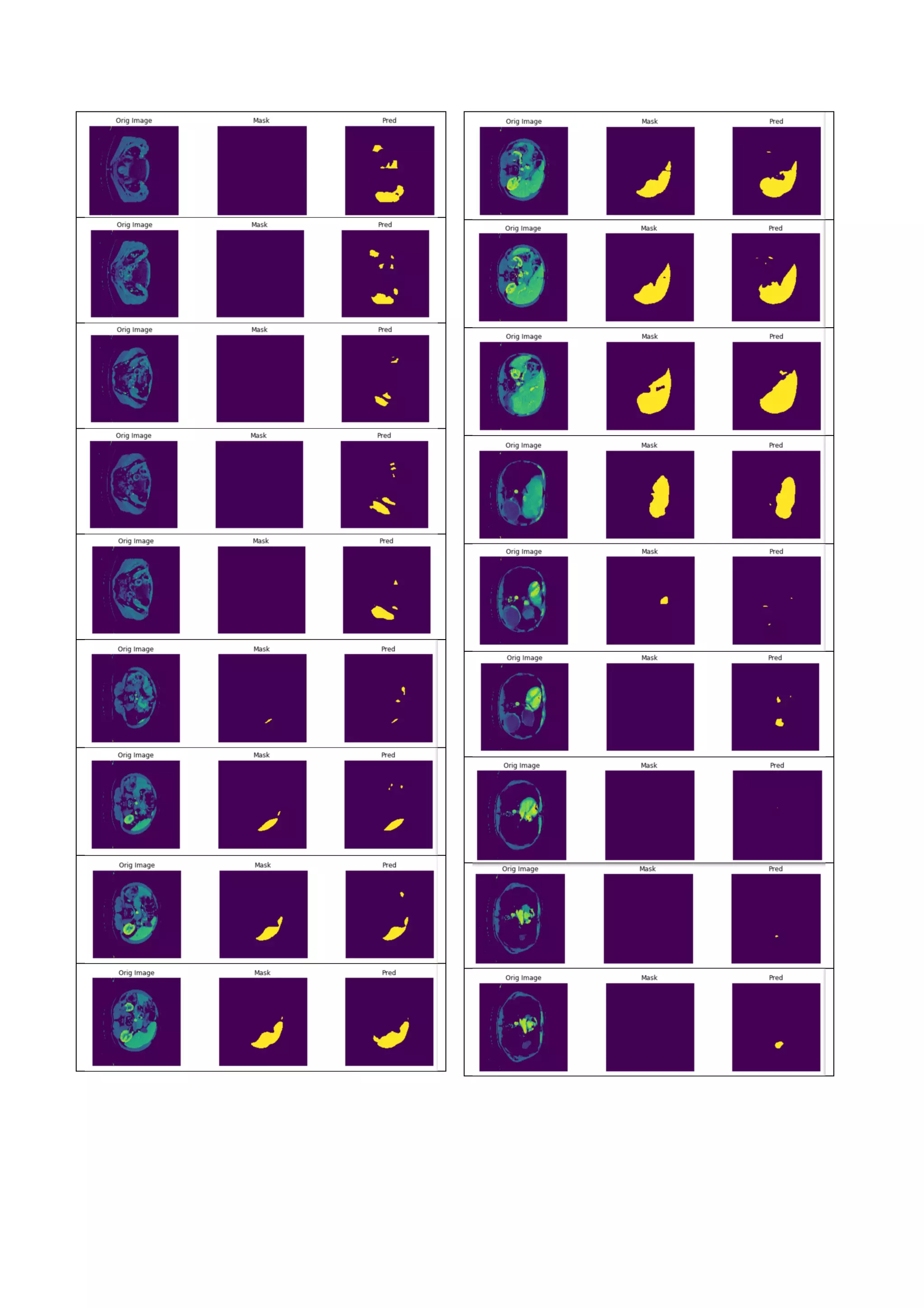
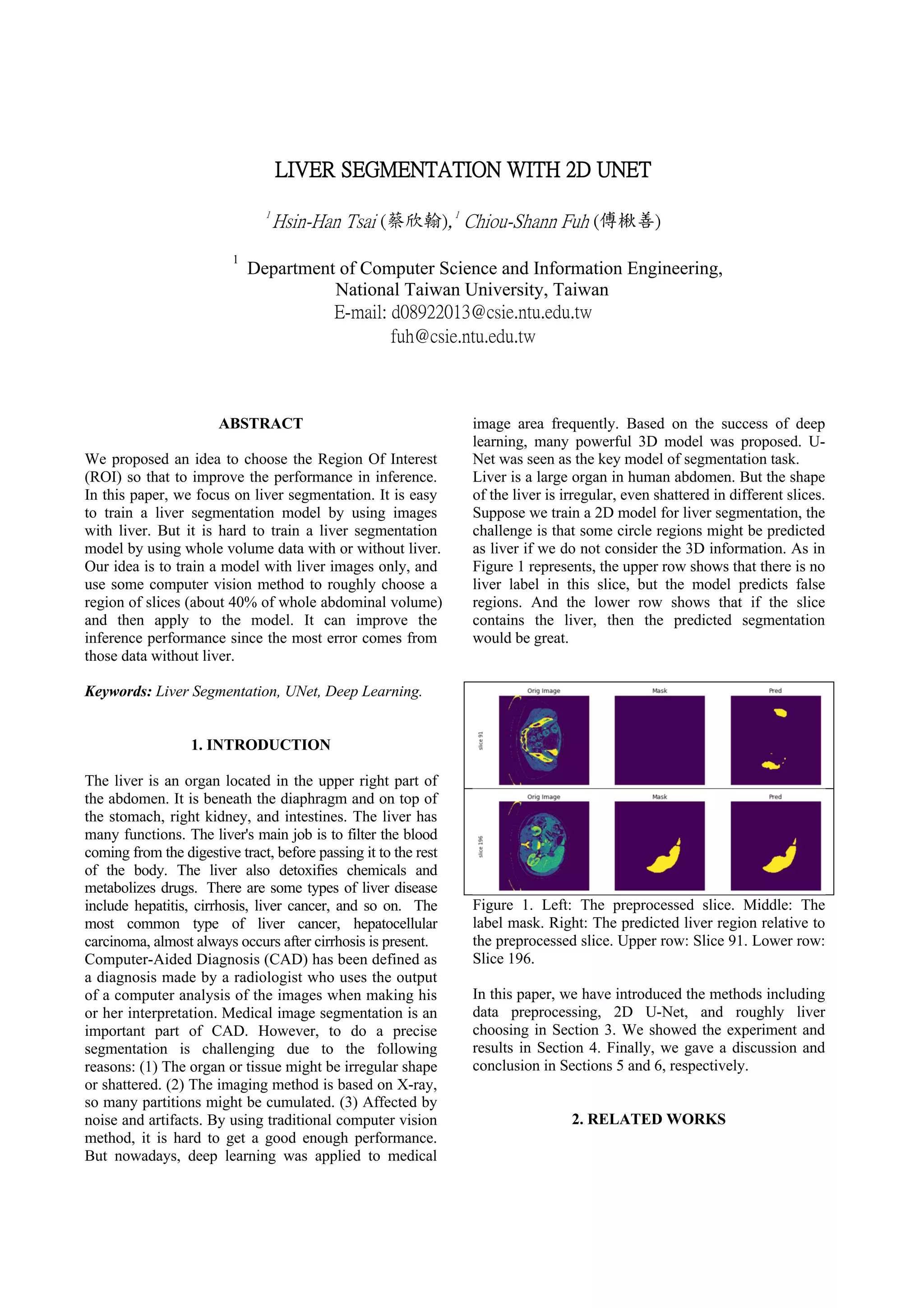
8. Figure 16. Compare of the predicted liver region and the
ground truth mask. Each row represents different slice.
The left column shows the original image. The middle
column shows the ground truth mask. And the right
column shows the predicted liver region.
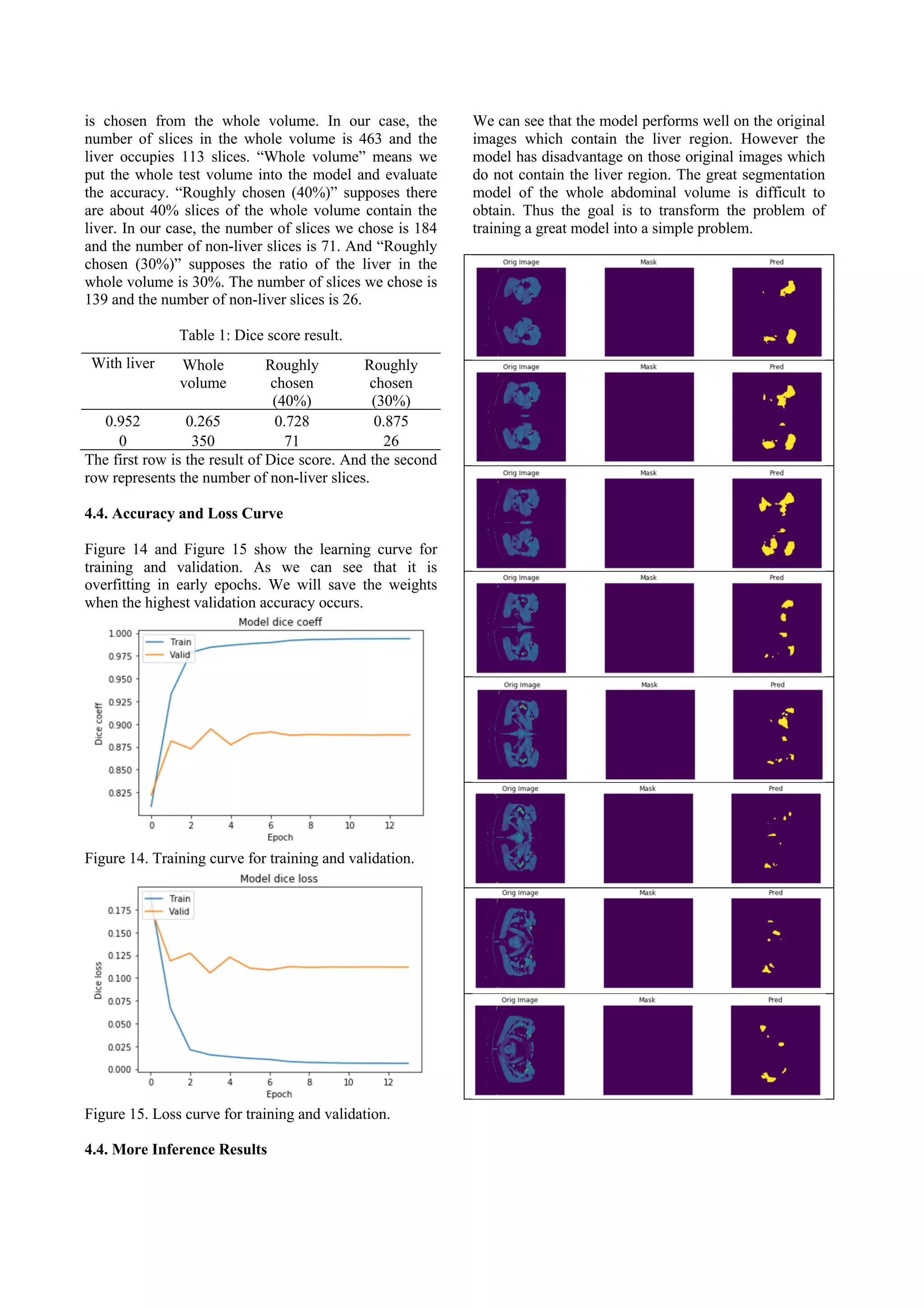
5. DISCUSSION
It seems that the roughly liver choosing method can help
to improve the accuracy. But it is still not good enough,
the roughly chosen (40%) contains 113 slices with liver
and also 71 slices without liver. In the other testing, the
roughly chosen (30%) contains 113 slices with liver and
also 26 slices without liver. The performance improves
significantly. So how to precisely get the range of slices
that contains liver becomes an important issue. For now,
we can find out the slice that contains the largest liver.
But we have not found some better methods based on
statistic or computer vision to choose the slices that
contain liver.
6. CONCLUSION
We proposed an idea to let the model focus on doing
liver segmentation on the images that contain liver.
And to choose the range that probably contain the liver
of the volume before inference. The tradeoff here is that
if we include more slices, we can ensure that the region
contains the liver. But if we include fewer slices, we
might not include the complete liver. The accuracy will
fall down since the unselected slices would be
considered as no liver. To include some 3D information
and use computer vision methods may help to choose
slices more accurate.
REFERENCES
[1] P. Bilic, P. F. Christ, E. Vorontsov, G. Chlebus, H. Chen,
Q. Dou, C. W. Fu, X. Han, P. A. Heng, J. Hesser, S.
Kadoury, T. Konopczynski, M. Le, C. Li, X. Li, J. Lipkovà,
J. Lowengrub, H. Meine, J. H. Moltz, C. Pal, M. Piraud, X.
Qi, J. Qi, M. Rempfler, K. Roth, A. Schenk, A.
Sekuboyina, E. Vorontsov, P. Zhou, C. Hülsemeyer, M.
Beetz, F. Ettlinger, F. Gruen, G. Kaissis, F. Lohöfer, R.
Braren, J. Holch, F. Hofmann, W. Sommer, V. Heinemann,
C. Jacobs, G. E. H. Mamani, B. v. Ginneken, G. Chartrand,
A. Tang, M. Drozdzal, A. Ben-Cohen, E. Klang, M. M.
Amitai, . Konen, H. Greenspan, J. Moreau, A. Hostettler, .
Soler, R. Vivanti, A. Szeskin, N. Lev-Cohain, J. Sosna, L.
Joskowicz, B. H. Menze, “The Liver Tumor Segmentation
Benchmark (LiTS),” CoRR, vol.abs/1901.04056, 2019.
[2] Christ, Patrick Ferdinand and Elshaer, Mohamed Ezzeldin
A. and Ettlinger, Florian and Tatavarty, Sunil and Bickel,
Marc and Bilic, Patrick and Rempfler, Markus and
Armbruster, Marco and Hofmann, Felix and D’Anastasi,
Melvin and et al., Automatic Liver and Lesion
Segmentation in CT Using Cascaded Fully Convolutional
Neural Networks and 3D Conditional Random Fields,
Springer International Publishing, 2016.
[3] X. Li, C. Huang, F. Jia, Z. Li, C. Fang, Y. Fan, Automatic
liver segmentation using statistical prior models and free-
form deformation, in: International MICCAI Workshop on
Medical Computer Vision, Springer, 2014, pp. 181–188.
[4] L. Rusko, G. Bekes, G. Nemeth, M. Fidrich, Fully
automatic liver segmentation for contrast-enhanced ct
images, MICCAI Wshp. 3D Segmentation in the Clinic: A
Grand Challenge 2 (7).
[5] A hybrid approach for liver segmentation, in:
Proceedings of MICCAI workshop on 3D
segmentation in the clinic: a grand challenge, 2007,
pp. 151–160.
[6] O. Ronneberger, P. Fischer, T. Brox, U-net: Convolutional
networks for biomedical image segmentation, in: MICCAI,
Vol. 9351, 2015, pp. 234–241.
[7] J. H. Moltz, L. Bornemann, V. Dicken, H. Peitgen,
Segmentation of liver metastases in ct scans by adaptive
thresholding and morphological processing, in: MICCAI
workshop, Vol. 41, 2008, p. 195.
[8] D. Wong, J. Liu, Y. Fengshou, Q. Tian, W. Xiong, J. Zhou,
Y. Qi, T. Han, S. Venkatesh, S.-c. Wang, A semi-
automated method for liver tumor segmentation based on
2d region growing with knowledge- based constraints, in:
MICCAI workshop, Vol. 41, 2008, p. 159.
[9] Y. Taieb, O. Eliassaf, M. Freiman, L. Joskowicz, J. Sosna,
An iterative bayesian approach for liver analysis: tumors
validation study, in: MICCAI workshop, Vol. 41, 2008, p.
43.
[10] I. Ben-Dan, E. Shenhav, Liver tumor segmentation in ct
images using probabilistic methods, in: MICCAI
Workshop, Vol. 41, 2008, p. 43.
[11] J. Stawiaski, E. Decenciere, F. Bidault, Interactive liver
tumor segmentation using graph-cuts and watershed, in:
Workshop on 3D Segmentation in the Clinic: A Grand
Challenge II. Liver Tumor Segmentation Challenge.
MICCAI, New York, USA, 2008.