Download free for 30 days
Sign in
Upload
Language (EN)
Support
Business
Mobile
Social Media
Marketing
Technology
Art & Photos
Career
Design
Education
Presentations & Public Speaking
Government & Nonprofit
Healthcare
Internet
Law
Leadership & Management
Automotive
Engineering
Software
Recruiting & HR
Retail
Sales
Services
Science
Small Business & Entrepreneurship
Food
Environment
Economy & Finance
Data & Analytics
Investor Relations
Sports
Spiritual
News & Politics
Travel
Self Improvement
Real Estate
Entertainment & Humor
Health & Medicine
Devices & Hardware
Lifestyle
Change Language
Language
English
Español
Português
Français
Deutsche
Cancel
Save
EN
Uploaded by
trahul9
PPT, PDF
10 views
Linear Regression in Machine Learning Notes for MCA.ppt
Linear Regression in Machine Learning Notes for MCA
Education
◦
Read more
0
Save
Share
Embed
Embed presentation
Download
Download to read offline
1
/ 85
2
/ 85
3
/ 85
4
/ 85
5
/ 85
6
/ 85
7
/ 85
8
/ 85
9
/ 85
10
/ 85
11
/ 85
12
/ 85
13
/ 85
14
/ 85
15
/ 85
16
/ 85
17
/ 85
18
/ 85
19
/ 85
20
/ 85
21
/ 85
22
/ 85
23
/ 85
24
/ 85
25
/ 85
26
/ 85
27
/ 85
28
/ 85
29
/ 85
30
/ 85
31
/ 85
32
/ 85
33
/ 85
34
/ 85
35
/ 85
36
/ 85
37
/ 85
38
/ 85
39
/ 85
40
/ 85
41
/ 85
42
/ 85
43
/ 85
44
/ 85
45
/ 85
46
/ 85
47
/ 85
48
/ 85
49
/ 85
50
/ 85
51
/ 85
52
/ 85
53
/ 85
54
/ 85
55
/ 85
56
/ 85
57
/ 85
58
/ 85
59
/ 85
60
/ 85
61
/ 85
62
/ 85
63
/ 85
64
/ 85
65
/ 85
66
/ 85
67
/ 85
68
/ 85
69
/ 85
70
/ 85
71
/ 85
72
/ 85
73
/ 85
74
/ 85
75
/ 85
76
/ 85
77
/ 85
78
/ 85
79
/ 85
80
/ 85
81
/ 85
82
/ 85
83
/ 85
84
/ 85
85
/ 85
More Related Content
PPT
Unit 4 SVM and AVR.ppt
by
Rahul Borate
PPT
svm-jain.ppt
by
shyam670838
PDF
2013-1 Machine Learning Lecture 05 - Andrew Moore - Support Vector Machines
by
Dongseo University
PPT
Support Vector Machines
by
nextlib
PPT
Support Vector Machine Lecture 2 For Machine Learning
by
mdshahariarhossain5
PPT
Introduction to Support Vector Machine 221 CMU.ppt
by
MuhammadImtiazHossai
PDF
Notes relating to Machine Learning and SVM
by
SyedSaimGardezi
PPT
SVM.ppt
by
SrikanthK799073
Unit 4 SVM and AVR.ppt
by
Rahul Borate
svm-jain.ppt
by
shyam670838
2013-1 Machine Learning Lecture 05 - Andrew Moore - Support Vector Machines
by
Dongseo University
Support Vector Machines
by
nextlib
Support Vector Machine Lecture 2 For Machine Learning
by
mdshahariarhossain5
Introduction to Support Vector Machine 221 CMU.ppt
by
MuhammadImtiazHossai
Notes relating to Machine Learning and SVM
by
SyedSaimGardezi
SVM.ppt
by
SrikanthK799073
Similar to Linear Regression in Machine Learning Notes for MCA.ppt
PPT
SvmHJ
by
rony122
PDF
Lecture4 xing
by
Tianlu Wang
PPT
SVM (2).ppt
by
NoorUlHaq47
PPTX
Machine learning interviews day2
by
rajmohanc
PPT
Support Vector Machine.ppt
by
NBACriteria2SICET
PPT
svm.ppt
by
RanjithaM32
PPT
support vector machine algorithm in machine learning
by
SamGuy7
PPT
lawper.ppt
by
HiuLXun4
PPT
support Vector Machine i Mathematics.ppt
by
TamilSelvi165
PPTX
Tutorial on Support Vector Machine
by
Loc Nguyen
PDF
Lecture 1: linear SVM in the primal
by
Stéphane Canu
PDF
OM-DS-Fall2022-Session10-Support vector machine.pdf
by
ssuserb016ab
PDF
Introduction to Support Vector Machines
by
Anish M M
PDF
Machine Learning Lectures -- Support Vector Machine (SVM)
by
Zahra Sadeghi
PPT
svm_introductory_ppt by university of texas
by
krutikavermafcs
PPT
Support vector MAchine using machine learning
by
GauravRaj772344
PPT
ai and ml presentation slides of svm.ppt
by
nishan252911
PDF
Gentle intro to SVM
by
Zoya Bylinskii
PDF
Support Vector Machines
by
guestfee8698
PPTX
SVMs.pptx support vector machines machine learning
by
AmgadAbdallah2
SvmHJ
by
rony122
Lecture4 xing
by
Tianlu Wang
SVM (2).ppt
by
NoorUlHaq47
Machine learning interviews day2
by
rajmohanc
Support Vector Machine.ppt
by
NBACriteria2SICET
svm.ppt
by
RanjithaM32
support vector machine algorithm in machine learning
by
SamGuy7
lawper.ppt
by
HiuLXun4
support Vector Machine i Mathematics.ppt
by
TamilSelvi165
Tutorial on Support Vector Machine
by
Loc Nguyen
Lecture 1: linear SVM in the primal
by
Stéphane Canu
OM-DS-Fall2022-Session10-Support vector machine.pdf
by
ssuserb016ab
Introduction to Support Vector Machines
by
Anish M M
Machine Learning Lectures -- Support Vector Machine (SVM)
by
Zahra Sadeghi
svm_introductory_ppt by university of texas
by
krutikavermafcs
Support vector MAchine using machine learning
by
GauravRaj772344
ai and ml presentation slides of svm.ppt
by
nishan252911
Gentle intro to SVM
by
Zoya Bylinskii
Support Vector Machines
by
guestfee8698
SVMs.pptx support vector machines machine learning
by
AmgadAbdallah2
More from trahul9
PPT
Computer System Architecture Notes for CS students Binary Codes.ppt
by
trahul9
PPT
Computer System Architecture Notes for Computer Science Students K-Maps.ppt
by
trahul9
PPT
Understanding 8085 Architecture( For computer science students).ppt
by
trahul9
PPT
Memory Hierarchy Notes of Computer Science students.ppt
by
trahul9
PPTX
Notes of Software Engineering for class MCA
by
trahul9
PPT
Digital Notes of Database Management System
by
trahul9
PPTX
Computer System Architecture Notes SEC-B.pptx
by
trahul9
PPTX
Computer System Architecture Notes SEC-A.pptx
by
trahul9
PPTX
Unit-4 Notes on Deep learning-compressed.pptx
by
trahul9
PPTX
Unit-4 Notes on Deep learning-compressed.pptx
by
trahul9
PPTX
Unit-3 Notes on deep Learning Machine Translation.pptx
by
trahul9
PPTX
Unit-3 Notes on deep Learning-compressed.pptx
by
trahul9
PPTX
Unit-3 deep Learning.pptx Notes of Deep Learning)
by
trahul9
PPTX
Unit-2 Structured.pptx( Notes of Deep Learning)
by
trahul9
PPTX
Linear Regression in Machine Learning Notes for MCA.pptx
by
trahul9
PPT
KNN and SVM algorithm in Machine Learning for MCA
by
trahul9
PPTX
KNN algorithm in Machine Learning for MCA
by
trahul9
PPTX
Machine Learning Notes on Decision Trees.pptx
by
trahul9
PPT
Lecture notes on Software Engineering MCA
by
trahul9
PPT
Notes on Understanding RDBMS2 for StudentsS.ppt
by
trahul9
Computer System Architecture Notes for CS students Binary Codes.ppt
by
trahul9
Computer System Architecture Notes for Computer Science Students K-Maps.ppt
by
trahul9
Understanding 8085 Architecture( For computer science students).ppt
by
trahul9
Memory Hierarchy Notes of Computer Science students.ppt
by
trahul9
Notes of Software Engineering for class MCA
by
trahul9
Digital Notes of Database Management System
by
trahul9
Computer System Architecture Notes SEC-B.pptx
by
trahul9
Computer System Architecture Notes SEC-A.pptx
by
trahul9
Unit-4 Notes on Deep learning-compressed.pptx
by
trahul9
Unit-4 Notes on Deep learning-compressed.pptx
by
trahul9
Unit-3 Notes on deep Learning Machine Translation.pptx
by
trahul9
Unit-3 Notes on deep Learning-compressed.pptx
by
trahul9
Unit-3 deep Learning.pptx Notes of Deep Learning)
by
trahul9
Unit-2 Structured.pptx( Notes of Deep Learning)
by
trahul9
Linear Regression in Machine Learning Notes for MCA.pptx
by
trahul9
KNN and SVM algorithm in Machine Learning for MCA
by
trahul9
KNN algorithm in Machine Learning for MCA
by
trahul9
Machine Learning Notes on Decision Trees.pptx
by
trahul9
Lecture notes on Software Engineering MCA
by
trahul9
Notes on Understanding RDBMS2 for StudentsS.ppt
by
trahul9
Recently uploaded
PDF
Chapter 05 Drug Acting on CNS General Anasthetics.pdf
by
SandeshSul
PPTX
MEMORY &FORGETTING. Shilpa Hotakar.Psychology pptx
by
SHILPA HOTAKAR
PPTX
A detailed notes on Conjugate Vaccine and its mechanism.
by
Dr. R. Ram
PDF
Artificial Intelligence in Research and Academic Writing, Workshop on Researc...
by
Prof. Vinod Kumar Kanvaria
PDF
Why Projects Fail – The Need to “Do the Right Project” and “Do the Project Ri...
by
Association for Project Management
PDF
Using T-Test to Analyze Research Data.pdf
by
Thelma Villaflores
PPTX
'Colonial Mentality and Social Identity in Karma by Khushwant Singh'
by
Krishnarajsinh Parmar
PPTX
How to Easily Track Appraisal Analysis Report in Odoo 18 Appraisal
by
Celine George
PPTX
West Hatch High School -- GCSE Geography
by
WestHatch
PPTX
ALTERNATIVE DV PROGRAMS Facilitator Training MAIN.pptx
by
Stephen Lasicka
PPTX
Reimagining Academic Library Services through Artificial Intelligence: A Case...
by
Don Bosco College, Itanagar
PDF
Unit Plan and Unit Test-pdf-Dr. Rajashekhar Shirvalkar, Principal, SMRS B.Ed ...
by
Rajashekhar Shirvalkar
PPTX
SOLAR SYSTEM.pptx || The infinity solar system
by
mahadevdigital024
PPTX
A brief introduction to Minor vegetable crops.pptx
by
UmeshTimilsina1
PDF
Schrodinger's Capital Finals (SciBiz Quiz).pdf
by
Conquiztadors- the Quiz Society of Sri Venkateswara College
PPTX
How Physician Assistants in the USA Earn CME Credits Online.pptx
by
CME4Life
PPT
West Hatch High School - GCSE History Option
by
WestHatch
PDF
West Hatch High School - GCSE French Specification
by
WestHatch
PPTX
"Aristotle : Father Of Western Philosophy"
by
mitalbarathod28
PDF
Pratishta Educational Society., Courses & Opportunities
by
GanapathiVankudoth
Chapter 05 Drug Acting on CNS General Anasthetics.pdf
by
SandeshSul
MEMORY &FORGETTING. Shilpa Hotakar.Psychology pptx
by
SHILPA HOTAKAR
A detailed notes on Conjugate Vaccine and its mechanism.
by
Dr. R. Ram
Artificial Intelligence in Research and Academic Writing, Workshop on Researc...
by
Prof. Vinod Kumar Kanvaria
Why Projects Fail – The Need to “Do the Right Project” and “Do the Project Ri...
by
Association for Project Management
Using T-Test to Analyze Research Data.pdf
by
Thelma Villaflores
'Colonial Mentality and Social Identity in Karma by Khushwant Singh'
by
Krishnarajsinh Parmar
How to Easily Track Appraisal Analysis Report in Odoo 18 Appraisal
by
Celine George
West Hatch High School -- GCSE Geography
by
WestHatch
ALTERNATIVE DV PROGRAMS Facilitator Training MAIN.pptx
by
Stephen Lasicka
Reimagining Academic Library Services through Artificial Intelligence: A Case...
by
Don Bosco College, Itanagar
Unit Plan and Unit Test-pdf-Dr. Rajashekhar Shirvalkar, Principal, SMRS B.Ed ...
by
Rajashekhar Shirvalkar
SOLAR SYSTEM.pptx || The infinity solar system
by
mahadevdigital024
A brief introduction to Minor vegetable crops.pptx
by
UmeshTimilsina1
Schrodinger's Capital Finals (SciBiz Quiz).pdf
by
Conquiztadors- the Quiz Society of Sri Venkateswara College
How Physician Assistants in the USA Earn CME Credits Online.pptx
by
CME4Life
West Hatch High School - GCSE History Option
by
WestHatch
West Hatch High School - GCSE French Specification
by
WestHatch
"Aristotle : Father Of Western Philosophy"
by
mitalbarathod28
Pratishta Educational Society., Courses & Opportunities
by
GanapathiVankudoth
Linear Regression in Machine Learning Notes for MCA.ppt
1.
Nov 23rd, 2001 Copyright
© 2001, 2003, Andrew W. Moore Support Vector Machines Andrew W. Moore Professor School of Computer Science Carnegie Mellon University www.cs.cmu.edu/~awm awm@cs.cmu.edu 412-268-7599 Note to other teachers and users of these slides. Andrew would be delighted if you found this source material useful in giving your own lectures. Feel free to use these slides verbatim, or to modify them to fit your own needs. PowerPoint originals are available. If you make use of a significant portion of these slides in your own lecture, please include this message, or the following link to the source repository of Andrew’s tutorials: http://www.cs.cmu.edu/~awm/tutorials . Comments and corrections gratefully received. Slides Modified for Comp537, Spring, 2006, HKUST
2.
Copyright © 2001,
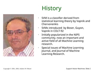
2003, Andrew W. Moore Support Vector Machines: Slide 2 History • SVM is a classifier derived from statistical learning theory by Vapnik and Chervonenkis • SVMs introduced by Boser, Guyon, Vapnik in COLT-92 • Initially popularized in the NIPS community, now an important and active field of all Machine Learning research. • Special issues of Machine Learning Journal, and Journal of Machine Learning Research.
3.
Copyright © 2001,
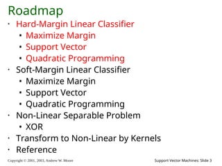
2003, Andrew W. Moore Support Vector Machines: Slide 3 Roadmap • Hard-Margin Linear Classifier • Maximize Margin • Support Vector • Quadratic Programming • Soft-Margin Linear Classifier • Maximize Margin • Support Vector • Quadratic Programming • Non-Linear Separable Problem • XOR • Transform to Non-Linear by Kernels • Reference
4.
Copyright © 2001,
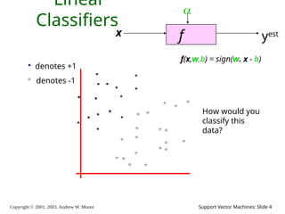
2003, Andrew W. Moore Support Vector Machines: Slide 4 Linear Classifiers f x yest denotes +1 denotes -1 f(x,w,b) = sign(w. x - b) How would you classify this data?
5.
Copyright © 2001,
2003, Andrew W. Moore Support Vector Machines: Slide 5 Linear Classifiers f x yest denotes +1 denotes -1 f(x,w,b) = sign(w. x - b) How would you classify this data?
6.
Copyright © 2001,
2003, Andrew W. Moore Support Vector Machines: Slide 6 Linear Classifiers f x yest denotes +1 denotes -1 f(x,w,b) = sign(w. x - b) How would you classify this data?
7.
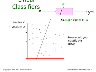
Copyright © 2001,
2003, Andrew W. Moore Support Vector Machines: Slide 7 Linear Classifiers f x yest denotes +1 denotes -1 f(x,w,b) = sign(w. x - b) How would you classify this data?
8.
Copyright © 2001,
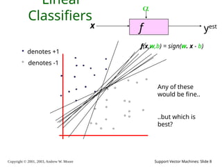
2003, Andrew W. Moore Support Vector Machines: Slide 8 Linear Classifiers f x yest denotes +1 denotes -1 f(x,w,b) = sign(w. x - b) Any of these would be fine.. ..but which is best?
9.
Copyright © 2001,
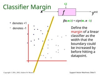
2003, Andrew W. Moore Support Vector Machines: Slide 9 Classifier Margin f x yest denotes +1 denotes -1 f(x,w,b) = sign(w. x - b) Define the margin of a linear classifier as the width that the boundary could be increased by before hitting a datapoint.
10.
Copyright © 2001,
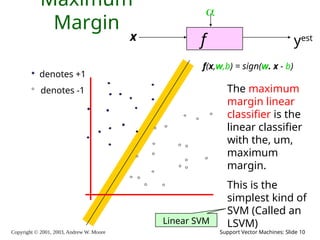
2003, Andrew W. Moore Support Vector Machines: Slide 10 Maximum Margin f x yest denotes +1 denotes -1 f(x,w,b) = sign(w. x - b) The maximum margin linear classifier is the linear classifier with the, um, maximum margin. This is the simplest kind of SVM (Called an LSVM) Linear SVM
11.
Copyright © 2001,
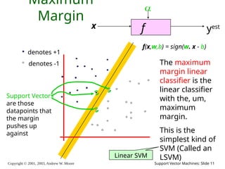
2003, Andrew W. Moore Support Vector Machines: Slide 11 Maximum Margin f x yest denotes +1 denotes -1 f(x,w,b) = sign(w. x - b) The maximum margin linear classifier is the linear classifier with the, um, maximum margin. This is the simplest kind of SVM (Called an LSVM) Support Vectors are those datapoints that the margin pushes up against Linear SVM
12.
Copyright © 2001,
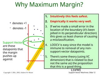
2003, Andrew W. Moore Support Vector Machines: Slide 12 Why Maximum Margin? denotes +1 denotes -1 f(x,w,b) = sign(w. x - b) The maximum margin linear classifier is the linear classifier with the, um, maximum margin. This is the simplest kind of SVM (Called an LSVM) Support Vectors are those datapoints that the margin pushes up against 1. Intuitively this feels safest. 2. Empirically it works very well. 3. If we’ve made a small error in the location of the boundary (it’s been jolted in its perpendicular direction) this gives us least chance of causing a misclassification. 4. LOOCV is easy since the model is immune to removal of any non- support-vector datapoints. 5. There’s some theory (using VC dimension) that is related to (but not the same as) the proposition that this is a good thing.
13.
Copyright © 2001,
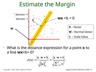
2003, Andrew W. Moore Support Vector Machines: Slide 13 Estimate the Margin • What is the distance expression for a point x to a line wx+b= 0? denotes +1 denotes -1 x wx +b = 0 2 2 1 2 ( ) d i i b b d w x w x w x w X – Vector W – Normal Vector b – Scale Value W
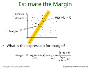
14.
Copyright © 2001,
2003, Andrew W. Moore Support Vector Machines: Slide 14 Estimate the Margin • What is the expression for margin? denotes +1 denotes -1 wx +b = 0 2 1 margin arg min ( ) arg min d D D i i b d w x x x w x Margin
15.
Copyright © 2001,
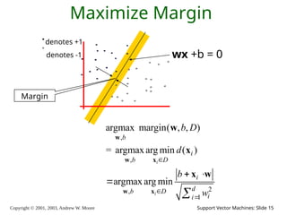
2003, Andrew W. Moore Support Vector Machines: Slide 15 Maximize Margin denotes +1 denotes -1 wx +b = 0 , , 2 , 1 argmax margin( , , ) = argmax arg min ( ) argmax arg min i i b i b D i d b D i i b D d b w w w x w x w x x w Margin
16.
Copyright © 2001,
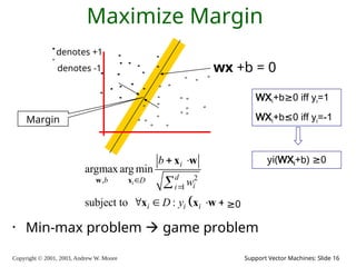
2003, Andrew W. Moore Support Vector Machines: Slide 16 Maximize Margin denotes +1 denotes -1 wx +b = 0 Margin • Min-max problem game problem WXi+b≥0 iff yi=1 WXi+b≤0 iff yi=-1 yi(WXi+b) ≥0 2 , 1 argmax arg min subject to : 0 i i d b D i i i i i b w D y b w x x w x x w ≥0
17.
Copyright © 2001,
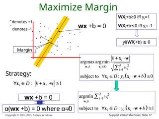
2003, Andrew W. Moore Support Vector Machines: Slide 17 Maximize Margin denotes +1 denotes -1 wx +b = 0 Margin Strategy: : 1 i i D b x x w 2 , 1 argmax arg min subject to : 0 i i d b D i i i i i b w D y b w x x w x x w 2 1 , argmin subject to : 1 d i i b i i i w D y b w x x w WXi+b≥0 iff yi=1 WXi+b≤0 iff yi=-1 yi(WXi+b) ≥ 0 wx +b = 0 α(wx +b) = 0 where α≠0
18.
Copyright © 2001,
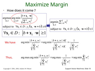
2003, Andrew W. Moore Support Vector Machines: Slide 18 Maximize Margin • How does it come ? : 1 i i D b x x w 2 , 1 argmax arg min subject to : 0 i i d b D i i i i i b w D y b w x x w x x w 2 1 , argmin subject to : 1 d i i b i i i w D y b w x x w d i i d i i i d i i i w K w K w x b w w x b 1 2 1 2 1 2 ' 1 | . | min arg | . | min arg d i i d i i d i i i w w w w x b 1 2 1 2 1 2 ' min arg ' 1 max arg | . | min arg max arg We have Thus,
19.
Copyright © 2001,
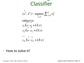
2003, Andrew W. Moore Support Vector Machines: Slide 19 Classifier • How to solve it? * * 2 1 , 1 1 2 2 { , }= argmax subject to 1 1 .... 1 d k k w b N N w b w y w x b y w x b y w x b
20.
Copyright © 2001,
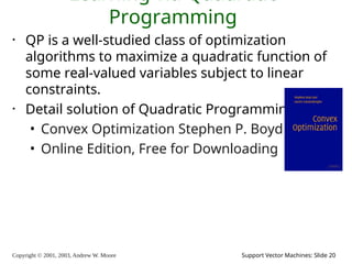
2003, Andrew W. Moore Support Vector Machines: Slide 20 Learning via Quadratic Programming • QP is a well-studied class of optimization algorithms to maximize a quadratic function of some real-valued variables subject to linear constraints. • Detail solution of Quadratic Programming • Convex Optimization Stephen P. Boyd • Online Edition, Free for Downloading
21.
Copyright © 2001,
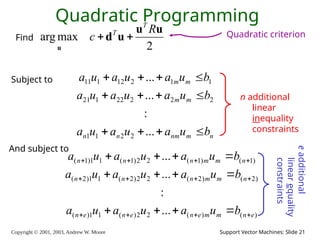
2003, Andrew W. Moore Support Vector Machines: Slide 21 Quadratic Programming 2 max arg u u u d u R c T T Find n m nm n n m m m m b u a u a u a b u a u a u a b u a u a u a ... : ... ... 2 2 1 1 2 2 2 22 1 21 1 1 2 12 1 11 ) ( ) ( 2 2 ) ( 1 1 ) ( ) 2 ( ) 2 ( 2 2 ) 2 ( 1 1 ) 2 ( ) 1 ( ) 1 ( 2 2 ) 1 ( 1 1 ) 1 ( ... : ... ... e n m m e n e n e n n m m n n n n m m n n n b u a u a u a b u a u a u a b u a u a u a And subject to n additional linear inequality constraints e additional linear equality constraints Quadratic criterion Subject to
22.
Copyright © 2001,
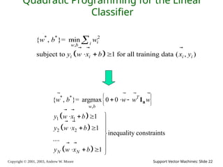
2003, Andrew W. Moore Support Vector Machines: Slide 22 Quadratic Programming for the Linear Classifier * * 2 , { , }= min subject to 1 for all training data ( , ) i i w b i i i i w b w y w x b x y * * , 1 1 2 2 { , }= argmax 0 0 1 1 inequality constraints .... 1 T w b N N w b w w w y w x b y w x b y w x b n I
23.
Copyright © 2001,
2003, Andrew W. Moore Support Vector Machines: Slide 23 Online Demo • Popular Tools - LibSVM
24.
Copyright © 2001,
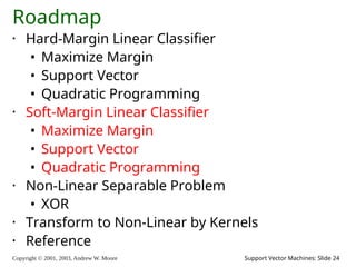
2003, Andrew W. Moore Support Vector Machines: Slide 24 Roadmap • Hard-Margin Linear Classifier • Maximize Margin • Support Vector • Quadratic Programming • Soft-Margin Linear Classifier • Maximize Margin • Support Vector • Quadratic Programming • Non-Linear Separable Problem • XOR • Transform to Non-Linear by Kernels • Reference
25.
Copyright © 2001,
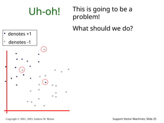
2003, Andrew W. Moore Support Vector Machines: Slide 25 Uh-oh! denotes +1 denotes -1 This is going to be a problem! What should we do?
26.
Copyright © 2001,
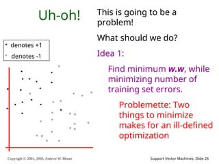
2003, Andrew W. Moore Support Vector Machines: Slide 26 Uh-oh! denotes +1 denotes -1 This is going to be a problem! What should we do? Idea 1: Find minimum w.w, while minimizing number of training set errors. Problemette: Two things to minimize makes for an ill-defined optimization
27.
Copyright © 2001,
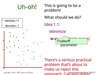
2003, Andrew W. Moore Support Vector Machines: Slide 27 Uh-oh! denotes +1 denotes -1 This is going to be a problem! What should we do? Idea 1.1: Minimize w.w + C (#train errors) There’s a serious practical problem that’s about to make us reject this Tradeoff parameter
28.
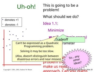
Copyright © 2001,
2003, Andrew W. Moore Support Vector Machines: Slide 28 Uh-oh! denotes +1 denotes -1 This is going to be a problem! What should we do? Idea 1.1: Minimize w.w + C (#train errors) There’s a serious practical problem that’s about to make us reject this Tradeoff parameter Can’t be expressed as a Quadratic Programming problem. Solving it may be too slow. (Also, doesn’t distinguish between disastrous errors and near misses) So… any other ideas?
29.
Copyright © 2001,
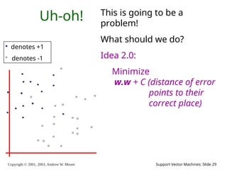
2003, Andrew W. Moore Support Vector Machines: Slide 29 Uh-oh! denotes +1 denotes -1 This is going to be a problem! What should we do? Idea 2.0: Minimize w.w + C (distance of error points to their correct place)
30.
Copyright © 2001,
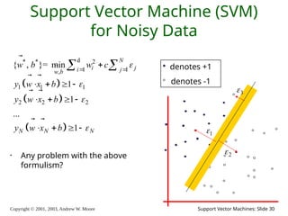
2003, Andrew W. Moore Support Vector Machines: Slide 30 Support Vector Machine (SVM) for Noisy Data • Any problem with the above formulism? d * * 2 1 1 , 1 1 1 2 2 2 { , }= min 1 1 ... 1 N i j i j w b N N N w b w c y w x b y w x b y w x b denotes +1 denotes -1 1 2 3
31.
Copyright © 2001,
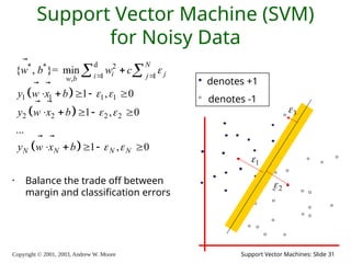
2003, Andrew W. Moore Support Vector Machines: Slide 31 Support Vector Machine (SVM) for Noisy Data • Balance the trade off between margin and classification errors d * * 2 1 1 , 1 1 1 1 2 2 2 2 { , }= min 1 , 0 1 , 0 ... 1 , 0 N i j i j w b N N N N w b w c y w x b y w x b y w x b denotes +1 denotes -1 1 2 3
32.
Copyright © 2001,
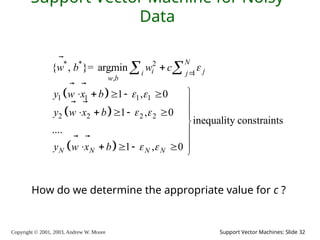
2003, Andrew W. Moore Support Vector Machines: Slide 32 Support Vector Machine for Noisy Data * * 2 1 , 1 1 1 1 2 2 2 2 { , }= argmin 1 , 0 1 , 0 inequality constraints .... 1 , 0 N i j i j w b N N N N w b w c y w x b y w x b y w x b How do we determine the appropriate value for c ?
33.
Copyright © 2001,
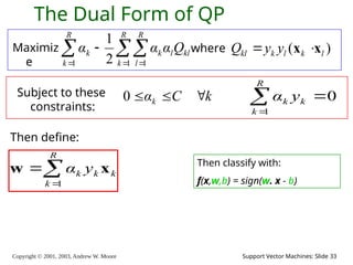
2003, Andrew W. Moore Support Vector Machines: Slide 33 The Dual Form of QP Maximiz e R k R l kl l k R k k Q α α α 1 1 1 2 1 where ( ) kl k l k l Q y y x x Subject to these constraints: k C αk 0 Then define: R k k k k y α 1 x w Then classify with: f(x,w,b) = sign(w. x - b) 0 1 R k k k y α
34.
Copyright © 2001,
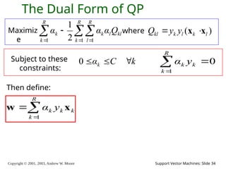
2003, Andrew W. Moore Support Vector Machines: Slide 34 The Dual Form of QP Maximiz e R k R l kl l k R k k Q α α α 1 1 1 2 1 where ( ) kl k l k l Q y y x x Subject to these constraints: k C αk 0 Then define: R k k k k y α 1 x w 0 1 R k k k y α
35.
Copyright © 2001,
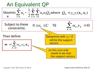
2003, Andrew W. Moore Support Vector Machines: Slide 35 An Equivalent QP Maximiz e where ) . ( l k l k kl y y Q x x Subject to these constraints: k C αk 0 Then define: R k k k k y α 1 x w 0 1 R k k k y α Datapoints with k > 0 will be the support vectors ..so this sum only needs to be over the support vectors. R k R l kl l k R k k Q α α α 1 1 1 2 1
36.
Copyright © 2001,
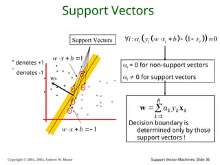
2003, Andrew W. Moore Support Vector Machines: Slide 36 Support Vectors denotes +1 denotes -1 1 w x b 1 w x b w Support Vectors Decision boundary is determined only by those support vectors ! R k k k k y α 1 x w : 1 0 i i i i i y w x b i = 0 for non-support vectors i 0 for support vectors
37.
Copyright © 2001,
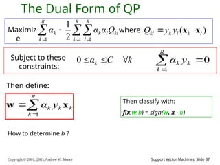
2003, Andrew W. Moore Support Vector Machines: Slide 37 The Dual Form of QP Maximiz e R k R l kl l k R k k Q α α α 1 1 1 2 1 where ( ) kl k l k l Q y y x x Subject to these constraints: k C αk 0 Then define: R k k k k y α 1 x w Then classify with: f(x,w,b) = sign(w. x - b) 0 1 R k k k y α How to determine b ?
38.
Copyright © 2001,
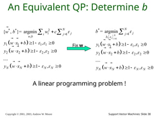
2003, Andrew W. Moore Support Vector Machines: Slide 38 An Equivalent QP: Determine b A linear programming problem ! * * 2 1 , 1 1 1 1 2 2 2 2 { , }= argmin 1 , 0 1 , 0 .... 1 , 0 N i j i j w b N N N N w b w c y w x b y w x b y w x b 1 * 1 , 1 1 1 1 2 2 2 2 = argmin 1 , 0 1 , 0 .... 1 , 0 N i i N j j b N N N N b y w x b y w x b y w x b Fix w
39.
Copyright © 2001,
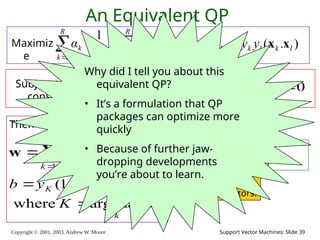
2003, Andrew W. Moore Support Vector Machines: Slide 39 R k R l kl l k R k k Q α α α 1 1 1 2 1 An Equivalent QP Maximiz e where ) . ( l k l k kl y y Q x x Subject to these constraints: k C αk 0 Then define: R k k k k y α 1 x w k k K K K K α K ε y b max arg where . ) 1 ( w x Then classify with: f(x,w,b) = sign(w. x - b) 0 1 R k k k y α Datapoints with k > 0 will be the support vectors ..so this sum only needs to be over the support vectors. Why did I tell you about this equivalent QP? • It’s a formulation that QP packages can optimize more quickly • Because of further jaw- dropping developments you’re about to learn.
40.
Copyright © 2001,
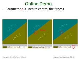
2003, Andrew W. Moore Support Vector Machines: Slide 40 Online Demo • Parameter c is used to control the fitness Noise
41.
Copyright © 2001,
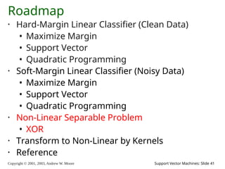
2003, Andrew W. Moore Support Vector Machines: Slide 41 Roadmap • Hard-Margin Linear Classifier (Clean Data) • Maximize Margin • Support Vector • Quadratic Programming • Soft-Margin Linear Classifier (Noisy Data) • Maximize Margin • Support Vector • Quadratic Programming • Non-Linear Separable Problem • XOR • Transform to Non-Linear by Kernels • Reference
42.
Copyright © 2001,
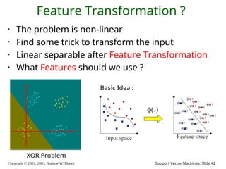
2003, Andrew W. Moore Support Vector Machines: Slide 42 Feature Transformation ? • The problem is non-linear • Find some trick to transform the input • Linear separable after Feature Transformation • What Features should we use ? XOR Problem Basic Idea :
43.
Copyright © 2001,
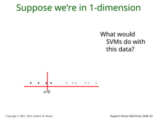
2003, Andrew W. Moore Support Vector Machines: Slide 43 Suppose we’re in 1-dimension What would SVMs do with this data? x=0
44.
Copyright © 2001,
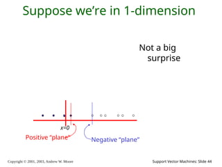
2003, Andrew W. Moore Support Vector Machines: Slide 44 Suppose we’re in 1-dimension Not a big surprise Positive “plane” Negative “plane” x=0
45.
Copyright © 2001,
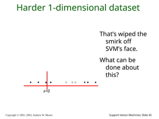
2003, Andrew W. Moore Support Vector Machines: Slide 45 Harder 1-dimensional dataset That’s wiped the smirk off SVM’s face. What can be done about this? x=0
46.
Copyright © 2001,
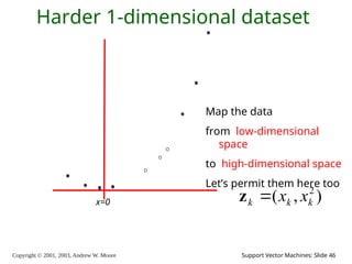
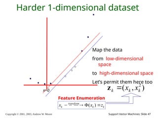
2003, Andrew W. Moore Support Vector Machines: Slide 46 Harder 1-dimensional dataset x=0 ) , ( 2 k k k x x z Map the data from low-dimensional space to high-dimensional space Let’s permit them here too
47.
Copyright © 2001,
2003, Andrew W. Moore Support Vector Machines: Slide 47 Harder 1-dimensional dataset Map the data from low-dimensional space to high-dimensional space Let’s permit them here too x=0 ) , ( 2 k k k x x z Feature Enumeration k k transform k z x x ) (
48.
Copyright © 2001,
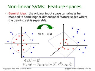
2003, Andrew W. Moore Support Vector Machines: Slide 48 Non-linear SVMs: Feature spaces • General idea: the original input space can always be mapped to some higher-dimensional feature space where the training set is separable: Φ: x → φ(x)
49.
Copyright © 2001,
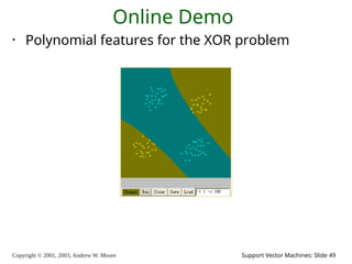
2003, Andrew W. Moore Support Vector Machines: Slide 49 Online Demo • Polynomial features for the XOR problem
50.
Copyright © 2001,
2003, Andrew W. Moore Support Vector Machines: Slide 50 Online Demo • But……Is it the best margin Intuitively?
51.
Copyright © 2001,
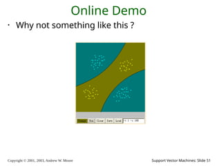
2003, Andrew W. Moore Support Vector Machines: Slide 51 Online Demo • Why not something like this ?
52.
Copyright © 2001,
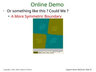
2003, Andrew W. Moore Support Vector Machines: Slide 52 Online Demo • Or something like this ? Could We ? • A More Symmetric Boundary
53.
Copyright © 2001,
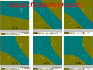
2003, Andrew W. Moore Support Vector Machines: Slide 53 Degree of Polynomial Features X^1 X^2 X^3 X^4 X^5 X^6
54.
Copyright © 2001,
2003, Andrew W. Moore Support Vector Machines: Slide 54 Towards Infinite Dimensions of Features ....... ! 4 1 ! 3 1 ! 2 1 ! 1 1 ! 1 4 3 2 1 0 x x x x x i e i i x • Enuermate polynomial features of all degrees ? • Taylor Expension of exponential function zk = ( radial basis functions of xk ) 2 2 | | exp ) ( ] [ j k k j k φ j c x x z
55.
Copyright © 2001,
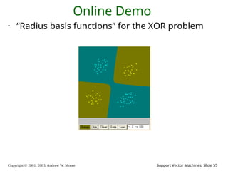
2003, Andrew W. Moore Support Vector Machines: Slide 55 Online Demo • “Radius basis functions” for the XOR problem
56.
Copyright © 2001,
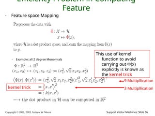
2003, Andrew W. Moore Support Vector Machines: Slide 56 Efficiency Problem in Computing Feature • Feature space Mapping • Example: all 2 degree Monomials 9 Multipllication 3 Multipllication kernel trick This use of kernel function to avoid carrying out Φ(x) explicitly is known as the kernel trick
57.
Copyright © 2001,
2003, Andrew W. Moore Support Vector Machines: Slide 57 Common SVM basis functions zk = ( polynomial terms of xk of degree 1 to q ) zk = ( radial basis functions of xk ) zk = ( sigmoid functions of xk ) 2 2 | | exp ) ( ] [ j k k j k φ j c x x z
58.
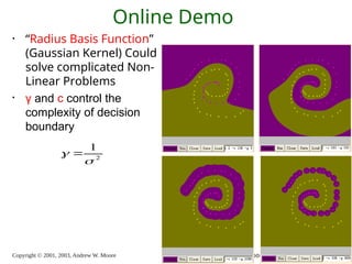
Copyright © 2001,
2003, Andrew W. Moore Support Vector Machines: Slide 58 Online Demo • “Radius Basis Function” (Gaussian Kernel) Could solve complicated Non- Linear Problems • γ and c control the complexity of decision boundary 2 1
59.
Copyright © 2001,
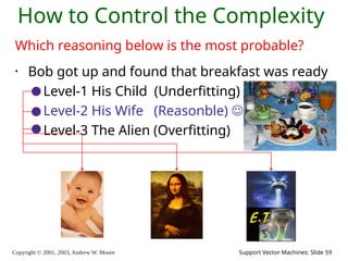
2003, Andrew W. Moore Support Vector Machines: Slide 59 How to Control the Complexity • Bob got up and found that breakfast was ready • Level-1 His Child (Underfitting) • Level-2 His Wife (Reasonble) • Level-3 The Alien (Overfitting) Which reasoning below is the most probable?
60.
Copyright © 2001,
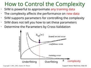
2003, Andrew W. Moore Support Vector Machines: Slide 60 How to Control the Complexity • SVM is powerful to approximate any training data • The complexity affects the performance on new data • SVM supports parameters for controlling the complexity • SVM does not tell you how to set these parameters • Determine the Parameters by Cross-Validation Underfitting Overfitting complexity
61.
Copyright © 2001,
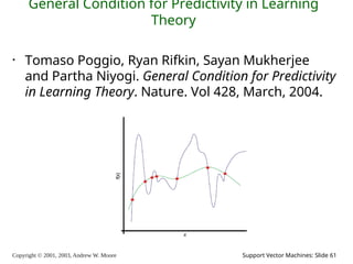
2003, Andrew W. Moore Support Vector Machines: Slide 61 General Condition for Predictivity in Learning Theory • Tomaso Poggio, Ryan Rifkin, Sayan Mukherjee and Partha Niyogi. General Condition for Predictivity in Learning Theory. Nature. Vol 428, March, 2004.
62.
Copyright © 2001,
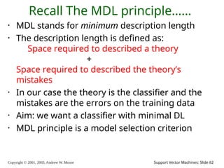
2003, Andrew W. Moore Support Vector Machines: Slide 62 Recall The MDL principle…… • MDL stands for minimum description length • The description length is defined as: Space required to described a theory + Space required to described the theory’s mistakes • In our case the theory is the classifier and the mistakes are the errors on the training data • Aim: we want a classifier with minimal DL • MDL principle is a model selection criterion
63.
Copyright © 2001,
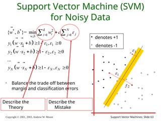
2003, Andrew W. Moore Support Vector Machines: Slide 63 Support Vector Machine (SVM) for Noisy Data • Balance the trade off between margin and classification errors d * * 2 1 1 , 1 1 1 1 2 2 2 2 { , }= min 1 , 0 1 , 0 ... 1 , 0 N i j i j w b N N N N w b w c y w x b y w x b y w x b denotes +1 denotes -1 1 2 3 Describe the Theory Describe the Mistake
64.
Copyright © 2001,
2003, Andrew W. Moore Support Vector Machines: Slide 64 SVM Performance • Anecdotally they work very very well indeed. • Example: They are currently the best-known classifier on a well-studied hand-written- character recognition benchmark • Another Example: Andrew knows several reliable people doing practical real-world work who claim that SVMs have saved them when their other favorite classifiers did poorly. • There is a lot of excitement and religious fervor about SVMs as of 2001. • Despite this, some practitioners are a little skeptical.
65.
Copyright © 2001,
2003, Andrew W. Moore Support Vector Machines: Slide 65 References • An excellent tutorial on VC-dimension and Support Vector Machines: C.J.C. Burges. A tutorial on support vector machines for pattern recognition. Data Mining and Knowledge Discovery, 2(2):955-974, 1998. http://citeseer.nj.nec.com/burges98tutorial.html • The VC/SRM/SVM Bible: (Not for beginners including myself) Statistical Learning Theory by Vladimir Vapnik, Wiley- Interscience; 1998 • Software: SVM-light, http://svmlight.joachims.org/, LibSVM, http://www.csie.ntu.edu.tw/~cjlin/libsvm/ SMO in Weka
66.
Nov 23rd, 2001 Copyright
© 2001, 2003, Andrew W. Moore Support Vector Regression
67.
Copyright © 2001,
2003, Andrew W. Moore Support Vector Machines: Slide 67 Roadmap • Squared-Loss Linear Regression • Little Noise • Large Noise • Linear-Loss Function • Support Vector Regression
68.
Copyright © 2001,
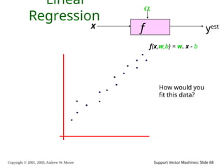
2003, Andrew W. Moore Support Vector Machines: Slide 68 Linear Regression f x yest f(x,w,b) = w. x - b How would you fit this data?
69.
Copyright © 2001,
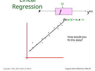
2003, Andrew W. Moore Support Vector Machines: Slide 69 Linear Regression f x yest f(x,w,b) = w. x - b How would you fit this data?
70.
Copyright © 2001,
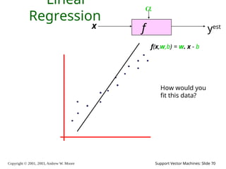
2003, Andrew W. Moore Support Vector Machines: Slide 70 Linear Regression f x yest f(x,w,b) = w. x - b How would you fit this data?
71.
Copyright © 2001,
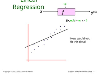
2003, Andrew W. Moore Support Vector Machines: Slide 71 Linear Regression f x yest f(x,w,b) = w. x - b How would you fit this data?
72.
Copyright © 2001,
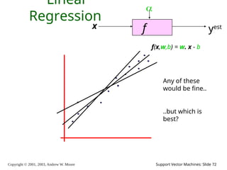
2003, Andrew W. Moore Support Vector Machines: Slide 72 Linear Regression f x yest f(x,w,b) = w. x - b Any of these would be fine.. ..but which is best?
73.
Copyright © 2001,
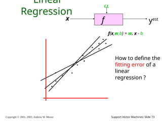
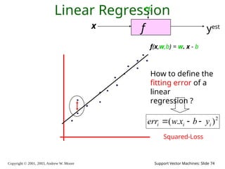
2003, Andrew W. Moore Support Vector Machines: Slide 73 Linear Regression f x yest f(x,w,b) = w. x - b How to define the fitting error of a linear regression ?
74.
Copyright © 2001,
2003, Andrew W. Moore Support Vector Machines: Slide 74 Linear Regression f x yest f(x,w,b) = w. x - b How to define the fitting error of a linear regression ? 2 ) . ( i i i y b x w err Squared-Loss
75.
Copyright © 2001,
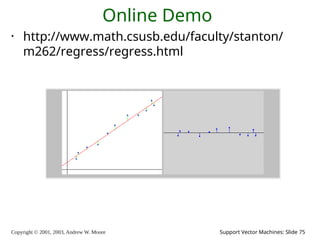
2003, Andrew W. Moore Support Vector Machines: Slide 75 Online Demo • http://www.math.csusb.edu/faculty/stanton/ m262/regress/regress.html
76.
Copyright © 2001,
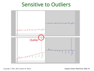
2003, Andrew W. Moore Support Vector Machines: Slide 76 Sensitive to Outliers Outlier
77.
Copyright © 2001,
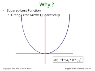
2003, Andrew W. Moore Support Vector Machines: Slide 77 Why ? • Squared-Loss Function • Fitting Error Grows Quadratically 2 ) . ( i i i y b x w err
78.
Copyright © 2001,
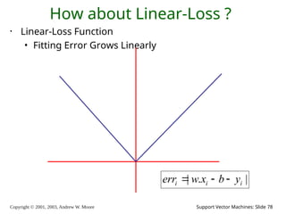
2003, Andrew W. Moore Support Vector Machines: Slide 78 How about Linear-Loss ? • Linear-Loss Function • Fitting Error Grows Linearly | . | i i i y b x w err
79.
Copyright © 2001,
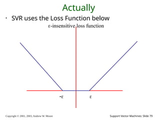
2003, Andrew W. Moore Support Vector Machines: Slide 79 Actually • SVR uses the Loss Function below -insensitive loss function
80.
Copyright © 2001,
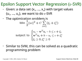
2003, Andrew W. Moore Support Vector Machines: Slide 80 Epsilon Support Vector Regression (-SVR) • Given: a data set {x1, ..., xn} with target values {u1, ..., un}, we want to do -SVR • The optimization problem is • Similar to SVM, this can be solved as a quadratic programming problem
81.
Copyright © 2001,
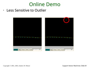
2003, Andrew W. Moore Support Vector Machines: Slide 81 Online Demo • Less Sensitive to Outlier
82.
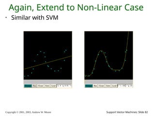
Copyright © 2001,
2003, Andrew W. Moore Support Vector Machines: Slide 82 Again, Extend to Non-Linear Case • Similar with SVM
83.
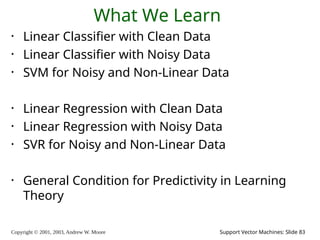
Copyright © 2001,
2003, Andrew W. Moore Support Vector Machines: Slide 83 What We Learn • Linear Classifier with Clean Data • Linear Classifier with Noisy Data • SVM for Noisy and Non-Linear Data • Linear Regression with Clean Data • Linear Regression with Noisy Data • SVR for Noisy and Non-Linear Data • General Condition for Predictivity in Learning Theory
84.
Copyright © 2001,
2003, Andrew W. Moore Support Vector Machines: Slide 84 The End
85.
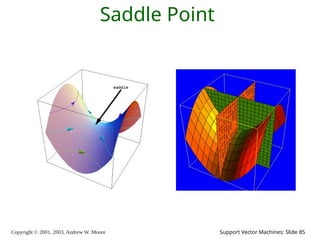
Copyright © 2001,
2003, Andrew W. Moore Support Vector Machines: Slide 85 Saddle Point
Download


![Copyright © 2001, 2003, Andrew W. Moore Support Vector Machines: Slide 54
Towards Infinite Dimensions of
Features
.......
!
4
1
!
3
1
!
2
1
!
1
1
!
1 4
3
2
1
0
x
x
x
x
x
i
e
i
i
x
• Enuermate polynomial features of all degrees ?
• Taylor Expension of exponential function
zk = ( radial basis functions of xk )
2
2
|
|
exp
)
(
]
[
j
k
k
j
k φ
j
c
x
x
z](https://image.slidesharecdn.com/comp537svm-new-250813110414-6b86212c/85/Linear-Regression-in-Machine-Learning-Notes-for-MCA-ppt-54-320.jpg)
![Copyright © 2001, 2003, Andrew W. Moore Support Vector Machines: Slide 57
Common SVM basis functions
zk = ( polynomial terms of xk of degree 1 to q )
zk = ( radial basis functions of xk )
zk = ( sigmoid functions of xk )
2
2
|
|
exp
)
(
]
[
j
k
k
j
k φ
j
c
x
x
z](https://image.slidesharecdn.com/comp537svm-new-250813110414-6b86212c/85/Linear-Regression-in-Machine-Learning-Notes-for-MCA-ppt-57-320.jpg)