Flair furniture LPP problem

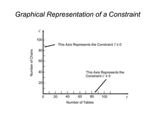
Graphical Representation of a Constraint
–
80 –
–
60 –
–
40 –
–
20 –
–
C
100 –
0 20 100
|– | | | | | | | | | | |
40 60 80
Number of Tables
T
Number
of
Chairs
This Axis Represents the Constraint T ≥ 0
This Axis Represents the
Constraint C ≥ 0

When Flair produces no tables, the carpentry
constraint is
4(0) + 3C = 240
3C = 240
C = 80
Similarly for no chairs
4T + 3(0) = 240
4T = 240
T = 60
line is shown on the following graph

100 –
–
80 –
–
60 –
–
40 –
–
20 –
–
C
0 20 100
|– | | | | | | | | | | |
40 60 80
Number of Tables
T
Number
of
Chairs
(T = 0, C = 80)
(T = 60, C = 0)
Graph of carpentry constraint equation

100 –
–
80 –
–
60 –
–
40 –
–
20 –
–
C
| | | | | | |
0 60 80 100 T
Number
of
Chairs
Number of Tables
Any point on or below the constraint plot
will not violate the restrictionAny point
above the plot will violate the restriction
(30, 40)
(30, 20)
|– | | | |
20 40
(70, 40)

The point (30, 40) lies on the plot and exactly
satisfies the constraint
4(30) + 3(40) = 240
The point (30, 20) lies below the plot and
satisfies the constraint
4(30) + 3(20) = 180
The point (30, 40) lies above the plot and
does not satisfy the constraint
4(70) + 3(40) = 400

100 –
–
80 –
–
60 –
–
40 –
–
20 –
–
C
0 20 100
|– | | | | | | | | | | |
40 60 80
Number of Tables
T
Number
of
Chairs
(T = 0, C = 100)
(T = 50, C = 0)
Graph of painting and varnishing
constraint equation

To produce tables and chairs, both departments
must be used
We need to find a solution that satisfies both
constraints simultaneously
A new graph shows both constraint plots
The feasible region (or area of feasible solutions) is
where all constraints are satisfied
Any point inside this region is a feasible solution
Any point outside the region is an infeasible
solution

100 –
–
80 –
–
60 –
–
40 –
–
20 –
–
C
0 100
| | | | | | | |
40 60 80
Number of Tables
T
Number
of
Chairs Feasible solution region for Flair Furniture
Painting/Varnishing Constraint
Carpentry Constraint
Feasible
Region
|– | | |
20

For the point (30, 20)
Carpentry
constraint
4T + 3C ≤ 240 hours available
(4)(30) + (3)(20) = 180 hours used
(2)(30) + (1)(20) = 80 hours used
Painting
constraint
Carpentry
constraint
(4)(70) + (3)(40) = 400 hours used
(2)(70) + (1)(40) = 180 hours used
Painting
constraint

Carpentry
constraint
(4)(50) + (3)(5) = 215 hours used
(2)(50) + (1)(5) = 105 hours used
Painting
constraint

Isoprofit Line Solution Method
Once the feasible region has been graphed, we need to
find the optimal solution from the many possible solutions
The speediest way to do this is to use the isoprofit line
method
Starting with a small but possible profit value, we graph
the objective function
We move the objective function line in the direction of
increasing profit while maintaining the slope
The last point it touches in the feasible region is the
optimal solution

For Flair Furniture, choose a profit of $2,100
The objective function is then
$2,100 = 70T + 50C
Solving for the axis intercepts, we can draw the graph
This is obviously not the best possible solution
Further graphs can be created using larger profits
The further we move from the origin while maintaining
the slope and staying within the boundaries of the
feasible region, the larger the profit will be
The highest profit ($4,100) will be generated when the
isoprofit line passes through the point (30, 40)

100 –
–
80 –
–
–
20 –
–
C
0 20 100
|– | | | | | | | | | | |
40 60 80
Number of Tables
T
Number
of
Chairs
Isoprofit line at $2,100
$2,100 = $70T + $50C
(30, 0)
60 –
–(0, 42)
40 –

100 –
–
80 –
–
60 –
–
40 –
–
20 –
–
C
0 20 100
|– | | | | | | | | | | |
40 60 80
Number of Tables
T
Number
of
Chairs
Four isoprofit lines
$2,100 = $70T + $50C
$2,800 = $70T + $50C
$3,500 = $70T + $50C
$4,100 = $70T + $50C

100 –
–
80 –
–
60 –
–
40 –
–
20 –
–
C
0 20 100
|– | | | | | | | | | | |
40 60 80
Number of Tables
T
Number
of
Chairs Optimal solution to the
Flair Furniture problem
Optimal Solution Point
(T = 30, C = 40)
Maximum Profit Line
$4,100 = $70T + $50C

A second approach to solving LP problems
employs the corner point method
It involves looking at the profit at every corner
point of the feasible region
The mathematical theory behind LP is that the
optimal solution must lie at one of the corner
points, or extreme point, in the feasible region
For Flair Furniture, the feasible region is a
four-sided polygon with four corner points
labeled 1, 2, 3, and 4 on the graph
Corner Point Solution Method

100 –
–
80 –
–
60 –
–
40 –
–
20 –
–
C
|– | | | | | | | | | | |
0 20 40 60 80 100 T
Number
of
Chairs
Number of Tables
Four corner points of the
feasible region
1
2
3
4

Point 1 : (T = 0, C = 0) Profit = $70(0) + $50(0) = $0
Point 2 : (T = 0, C = 80) Profit = $70(0) + $50(80) = $4,000
Point 4 : (T = 50, C = 0) Profit = $70(50) + $50(0) = $3,500
Point 3 : (T = 30, C = 40) Profit = $70(30) + $50(40) = $4,100
Because Point
optimal solution
3 returns the highest profit, this is the
To find the coordinates for Point3 accurately we have to
solve for the intersection of the two constraint lines
The details of this are on the following slide

Using the simultaneous equations method, we multiply
the painting equation by –2 and add it to the carpentry
equation
4T + 3C = 240
– 4T – 2C =–200
C = 40
(carpentry line)
(painting line)
Substituting 40 for C in either of the original equations
allows us to determine the value of T
(carpentry line)
4T + (3)(40) = 240
4T + 120 = 240
T = 30

Summary of Graphical Solution Methods
ISOPROFIT METHOD
1. Graph all constraints and find the feasible region.
2. Select a specific profit (or cost) line and graph it to find the slope.
3. Move the objective function line in the direction of increasing profit (or decreasing
cost) while maintaining the slope. The last point it touches in the feasible region is
the optimal solution.
4. Find the values of the decision variables at this last point and compute the profit
(or cost).
CORNER POINT METHOD
1. Graph all constraints and find the feasible region.
2. Find the corner points of the feasible reason.
3. Compute the profit (or cost) at each of the feasible corner points.
4. select the corner point with the best value of the objective function found in Step 3.
This is the optimal solution.

Solving Minimization Problems
Many LP problems involve minimizing an
objective such as cost instead of maximizing a
profit function
Minimization problems can be solved
graphically by first setting up the feasible
solution region and then using either the
corner point method or an isocost line
approach (which is analogous to the isoprofit
approach in maximization problems) to find
the values of the decision variables (e.g., X1
and X2) that yield the minimum cost

5X1 + 10X2 ≥ 90 ounces
4X1 + 3X2 ≥ 48 ounces
0.5X1 ≥ 1.5 ounces
X1 ≥ 0
X2 ≥ 0
(ingredient constraint A)
(ingredient constraint B)
(ingredient constraint C)
(nonnegativity constraint)
(nonnegativity constraint)
The Holiday Meal Turkey Ranch is considering buying
two different brands of turkey feed and blending them
to provide a good, low-cost diet for its turkeys
Let
X1 = number of pounds of brand 1 feed purchased
X2 = number of pounds of brand 2 feed purchased
Minimize cost (in cents) = 2X1 + 3X2
subject to:
Holiday Meal Turkey Ranch

COMPOSITION OF EACH POUND
OF FEED (OZ.)
INGREDIENT BRAND 1 FEED BRAND 2 FEED
MINIMUM MONTHLY
REQUIREMENT PER
TURKEY (OZ.)
A 5 10 90
B 4 3 48
C 0.5 0 1.5
Cost per pound 2 cents 3 cents
Holiday Meal Turkey Ranch data

Using the corner
point method
First we construct the
feasible solution
region
The optimal solution
will lie at on of the
corners as it would in
a maximization
problem
20
15
10
5
0
X2
|
5 25
10 15 20
Pounds of Brand 1
X1
Pounds
of
Brand
2
–
|
Ingredient C Constraint
Feasible Region
Ingredient B Constraint
b Ingredient A Constraint
| | c | |
–
–
–
a
–
–
Figure 7.10

We solve for the values of the three corner points
Point a is the intersection of ingredient constraints C
and B
4X1 + 3X2 = 48
X1 = 3
Substituting 3 in the first equation, we find X2 = 12
Solving for point b with basic algebra we find X1 = 8.4
and X2 = 4.8
Solving for point c we find X1 = 18 and X2 = 0

Substituting these value back into the objective
function we find
Cost = 2X1 + 3X2
Cost at point a = 2(3) + 3(12) = 42
Cost at point b = 2(8.4) + 3(4.8) = 31.2
Cost at point c = 2(18) + 3(0) = 36
The lowest cost solution is to purchase 8.4 pounds of
brand 1 feed and 4.8 pounds of brand 2 feed for a
total cost of 31.2 cents per turkey

–
Using the isocost
approach
Choosing an initial 20 –
cost of 54 cents, it is
clear improvement
is possible
15 –
10 –
5 –
0 –
X2
| | | |
25 X1
Pounds
of
Brand
2
5 10 15 20
Pounds of Brand 1
Figure 7.11
Feasible Region
(X1 = 8.4, X2 = 4.8)
| |

Four Special Cases in LP
Four special cases and difficulties arise at
times when using the graphical approach to
solving LP problems
Infeasibility
Unboundedness
Redundancy
Alternate Optimal Solutions

No feasible solution
Exists when there is no solution to the problem that
satisfies all the constraint equations
No feasible solution region exists
This is a common occurrence in the real world
Generally one or more constraints are relaxed until
a solution is found

A problem with no feasible
solution
8 –
–
6 –
–
4 –
–
2 –
–
0 –
X2
| | | | | | | | | |
X1
2 4 6 8
Region Satisfying First Two Constraints
Region Satisfying
Third Constraint
X1+2X2 <=6
2X1+X2 <=8
X1 >=7

Unboundedness
Sometimes a linear program will not have a finite
solution
In a maximization problem, one or more solution
variables, and the profit, can be made infinitely large
without violating any constraints
In a graphical solution, the feasible region will be
open ended
This usually means the problem has been
formulated improperly

A solution region unbounded to the right
15
10
5
0
X2
5 10 15 X1
–
–
X1 ≥ 5
X2 ≤ 10
–
–
|
Feasible Region
X1 + 2X2 ≥ 15
| | | |

Redundancy
A redundant constraint is one that does not affect the
feasible solution region
One or more constraints may be more binding
This is a very common occurrence in the real
world
It causes no particular problems, but eliminating
redundant constraints simplifies the model

A problem with a
redundant
constraint
30 –
25 –
20 –
15 –
10 –
5 –
0 –
X2
| | | | | |
5 10 15 20 25 30 X1
Feasible
Region
Redundant
Constraint
X1 ≤ 25
2X1 + X2 ≤ 30
X1 + X2 ≤20

Alternate Optimal Solutions
Occasionally two or more optimal solutions may
exist
Graphically this occurs when the objective
function’s isoprofit or isocost line runs perfectly
parallel to one of the constraints
This actually allows management great flexibility in
deciding which combination to select as the profit is
the same at each alternate solution

Example of
alternate optimal
solutions 8 –
5 –
4 –
3 –
2 –
0 –
X2
| | | |
1 – Feasible
1 2 3
Region
Isoprofit Line for $8
Optimal Solution Consists of All
Combinations of X1 and X2 Along the
AB Segment
Isoprofit Line for $12
Overlays Line Segment AB
| | | |
4 5 6 7 8 X1
B
7 –
A
6 –
Maximize 3X1 + 2X2
Subj. To: 6X1 + 4X2 < 24
X1 < 3
X1, X2 > 0

Sensitivity Analysis
Optimal solutions to LP problems thus far have been
found under what are called deterministic assumptions
This means that we assume complete certainty in the
data and relationships of a problem
But in the real world, conditions are dynamic and
changing
We can analyze how sensitive a deterministic solution is
to changes in the assumptions of the model
This is called sensitivity analysis, postoptimality
analysis, parametric programming, or optimality
analysis

Sensitivity analysis often involves a series of what-if?
questions concerning constraints, variable
coefficients, and the objective function
What if the profit for product 1 increases by 10%?
What if less advertising money is available?
One way to do this is the trial-and-error method where
values are changed and the entire model is resolved.
The preferred way is to use an analytic postoptimality
analysis
After a problem has been solved, we determine a range
of changes in problem parameters that will not affect the
optimal solution or change the variables in the solution
without re-solving the entire problem

Sensitivity analysis can be used to deal not only
with errors in estimating input parameters to the
LP model but also with management’s
experiments with possible future changes in the
firm that may affect profits.

Flair furniture LPP problem

Recommended

Recommended

More Related Content

What's hot

What's hot (20)

Similar to Flair furniture LPP problem

Similar to Flair furniture LPP problem (20)

More from Karishma Chaudhary

More from Karishma Chaudhary (20)

Recently uploaded

Recently uploaded (20)

Flair furniture LPP problem