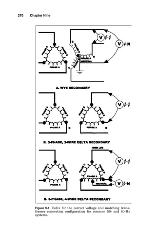
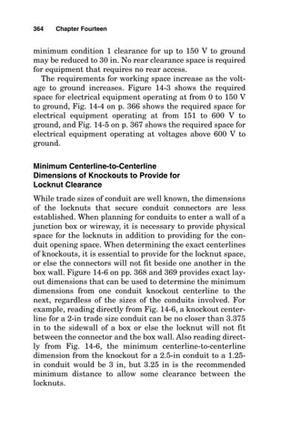
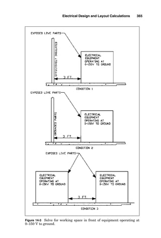
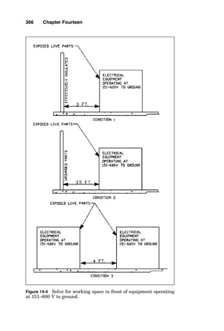
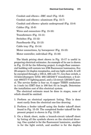
This document is the preface and table of contents for a handbook on electrical calculations by John M. Paschal Jr. P.E. The preface explains that the handbook aims to provide commonly needed electrical reference information, examples of typical calculations, and explanations of concepts in a single portable volume. The table of contents lists the chapters and problems covered in the handbook, ranging from basic electrical concepts to lighting, power systems, conductors, grounding, motors and more.
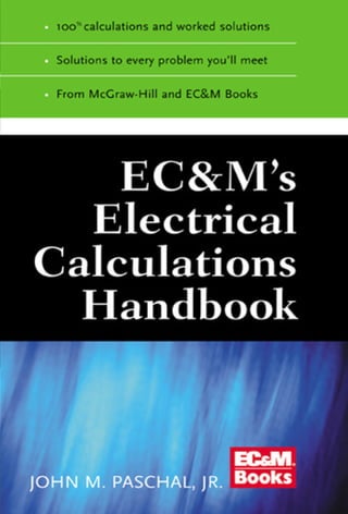


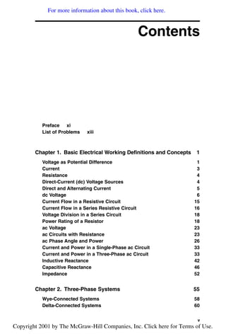
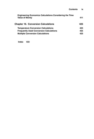


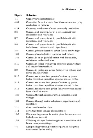

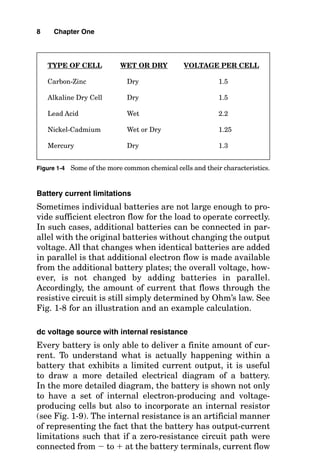
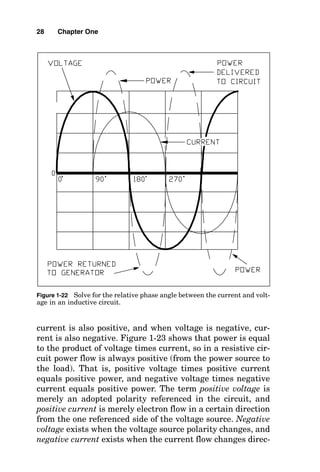
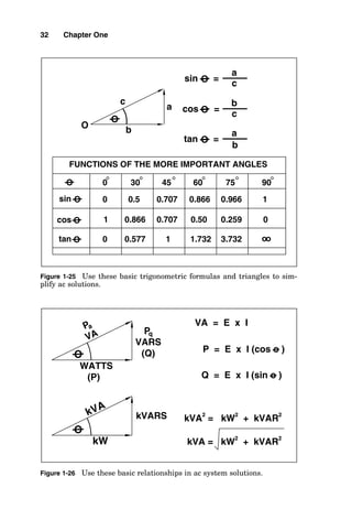
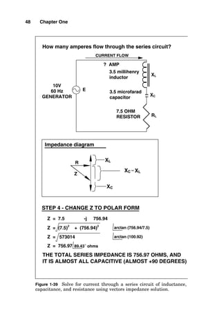
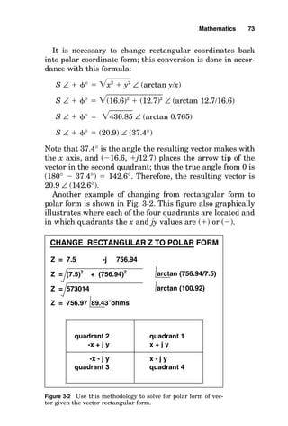
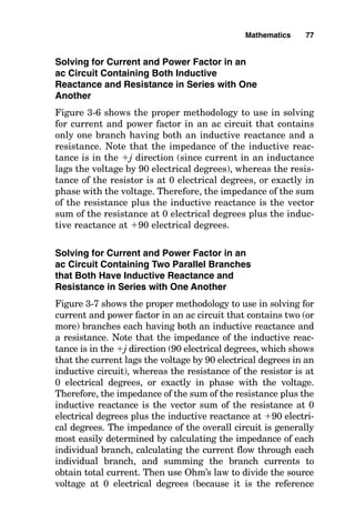
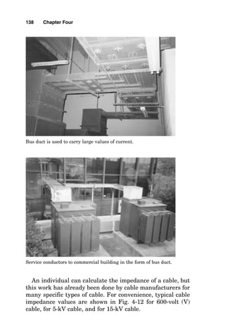
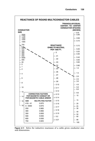
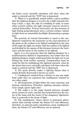
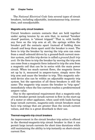
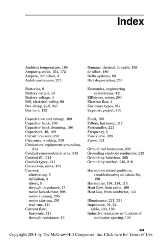
![Basic Electrical Working Definitions and Concepts 51
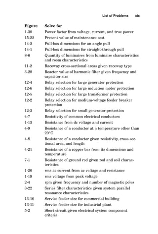
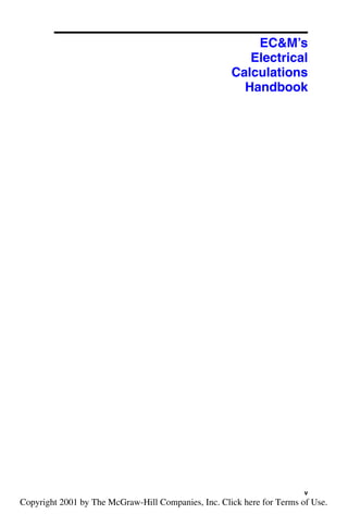
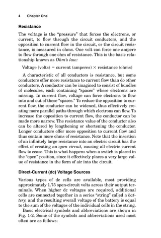
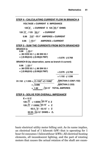
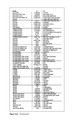
VOLTAGE = CURRENT X IMPEDANCE
0.96 AMPERES = CURRENT
120 = CURRENT X 125 OHMS
120 / 125 = CURRENT
0°
0.0° - 53.1°
53.1°
0° 53.1°
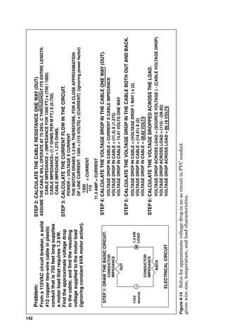
STEP 6 - CALCULATING CURRENT FLOW IN BRANCH A
0.96 AMPERES = CURRENT
- 53.1°
0.6 AMPERES = CURRENT
0.0° - (-90)°
120 / 200 = CURRENT
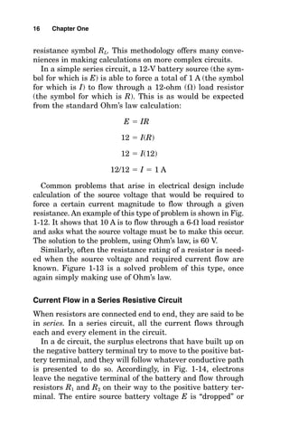
120 = CURRENT X 200 OHMS
STEP 7 - CALCULATING CURRENT FLOW IN BRANCH B
VOLTAGE = CURRENT X IMPEDANCE
0°
0° -90°
-90°
STEP 8 - CHANGE THE CURRENTS TO VECTOR VALUES,
AND THEN SUM THE CURRENTS FROM BOTH BRANCHES
0.96
= .96 COS -53.1 +j .96 SIN -53.1
= [ (0.96)(0.6) +j (0.96)(-0.7997)
- 53.1°
0.6
= .6 COS 90 +j 0.6SIN 90
= [(.6)(0) +j (0.6)(1)]
90°
= 0.576 -j 0.77
0.6 AMPERES = CURRENT
90°
= 0 +j 0.6
= 0.576 -j 0.17
BRANCH A
BRANCH B
0.576 -j 0.17 = (0.576)2
+ (0.17)2
- ARCTAN (0.17/0.576)
0.3307 - ARCTAN (0.2951)
0.6 -16.4° TOTAL AMPERES
STEP 9 - SOLVE FOR OVERALL IMPEDANCE
E = I X Z
120 = 0.6 X Z
0° -16.4°
120 / 0.6 = Z
0° -16.4°
200 = Z
0°- (-16.4°)
200 OHMS = ZT
16.4°](https://image.slidesharecdn.com/libro-electricalcalculationhandbook-220531173735-cc042810/85/LIBRO-Electrical-Calculation-HandBook-pdf-76-320.jpg)


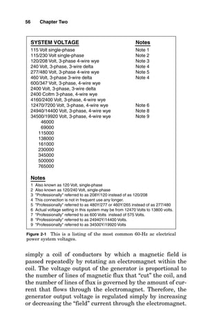
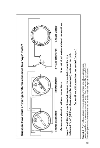
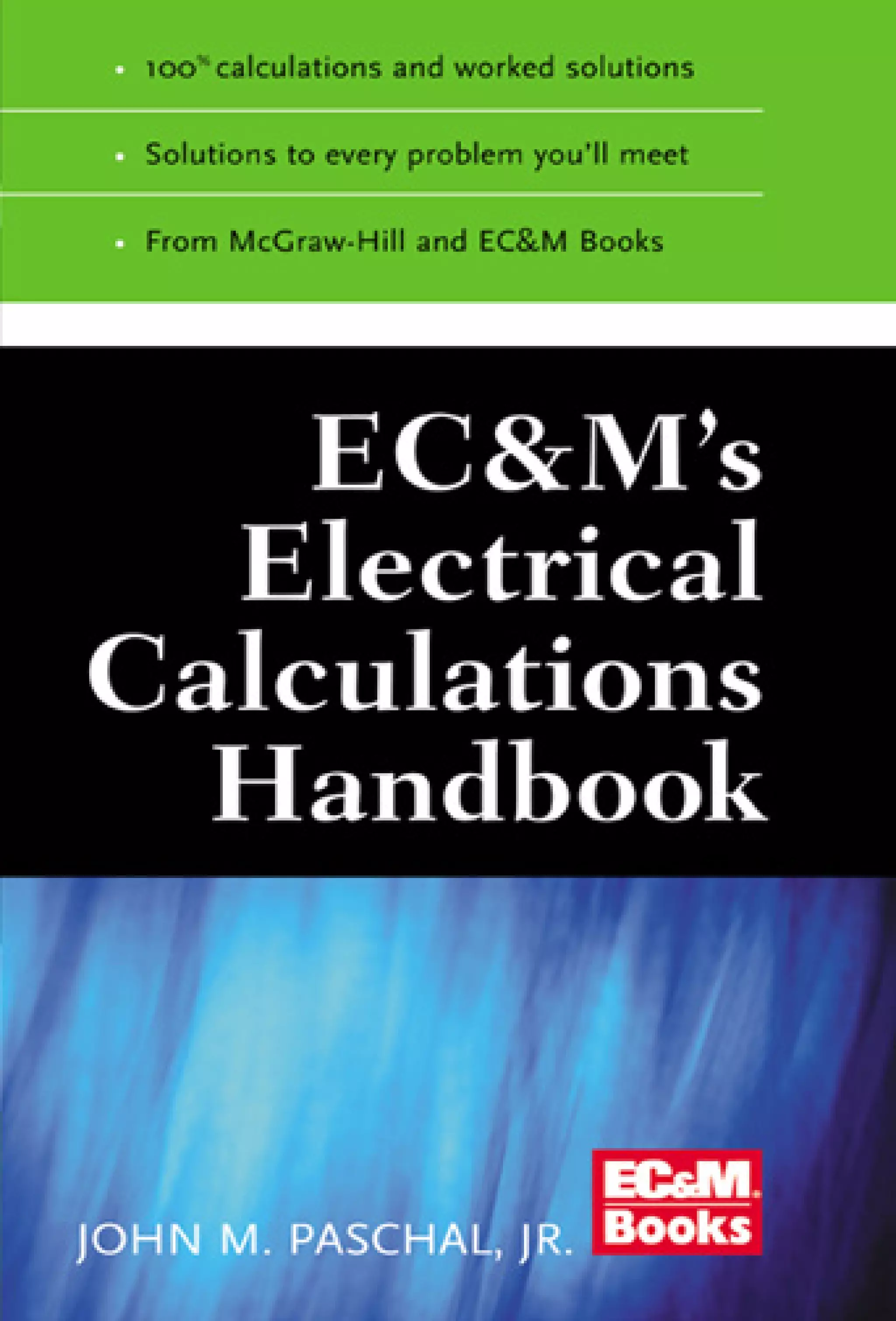
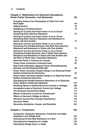
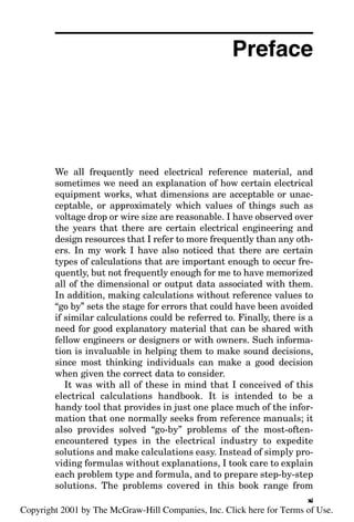
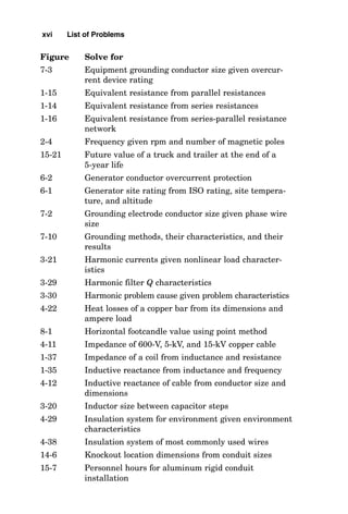
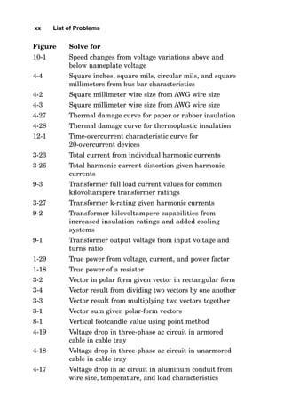
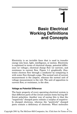
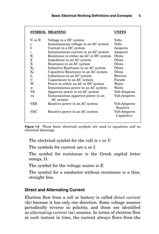
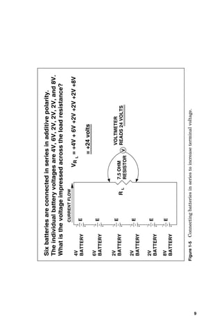
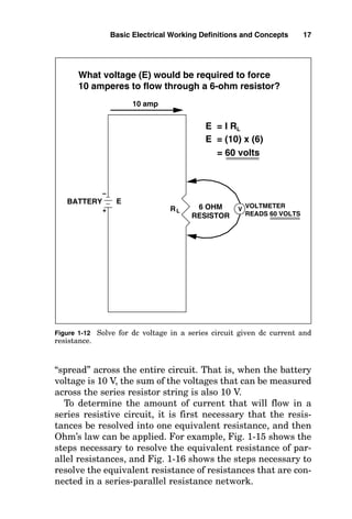
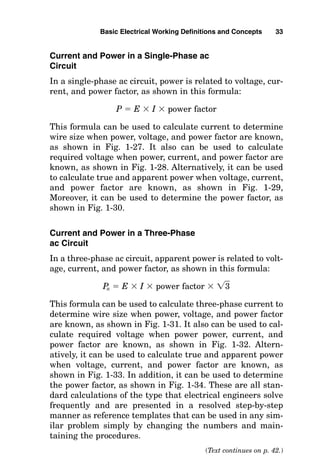
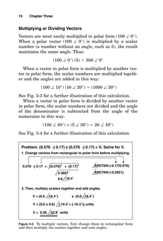
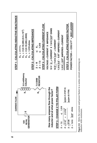
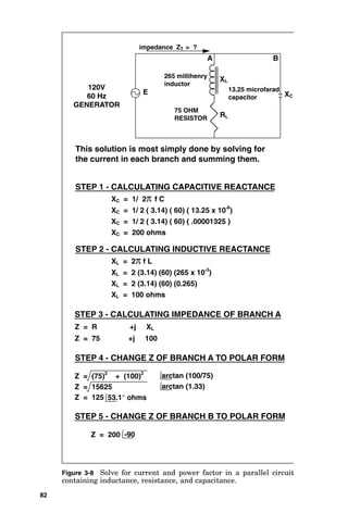
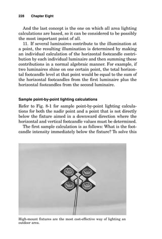
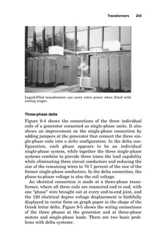
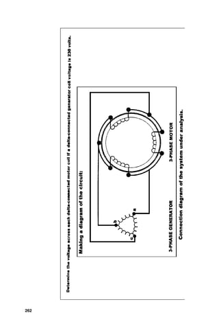
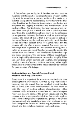
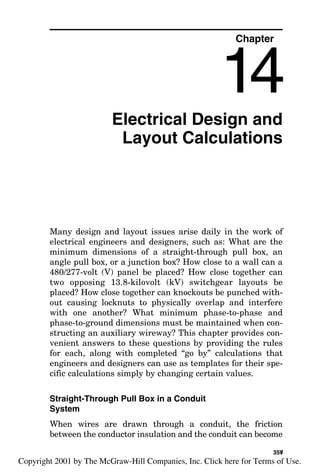
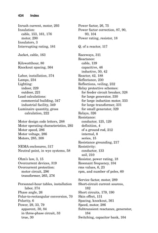
![3-PHASE
GENERATOR
3-PHASE
MOTOR
a
b
c
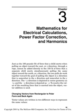
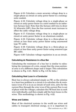
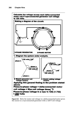
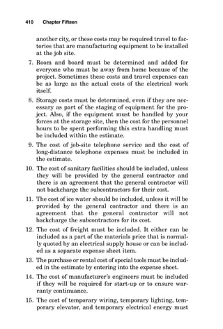
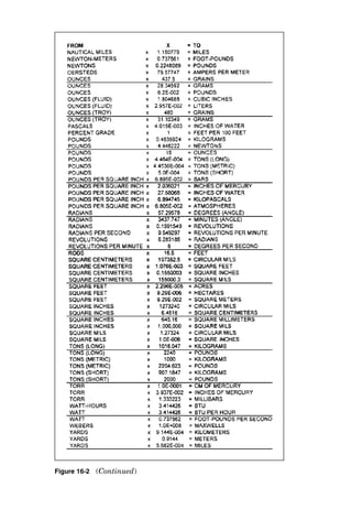
Calculate
the
voltage
across
each
delta-connected
motor
coil
if
wye-connected
generator
coil
voltage
is
120
volts.
n
180
-j
104
=
(180)
2
+
(104)
2
Minus
Phase
b
voltage
-
(120
120
°
=
-
120
-60
°
)
=
-(-120
COS
60
-j
120
SIN
60)
=
-[(-120)(5)
-j
(120)(.866)]
=
-[-60
+j
103.92]
Phase
a
voltage:
120
=
120
COS
0
+
j
120
SIN
0
=
[
(120)(1)
+j
(120)(0)]
0
°
=
+60
-j
104
ARCTAN
(-
0.577)
ARCTAN
(-104/180)
=
180
-j
104
=
120
+
j
0.0
+
30
°
-
180
°
=
208
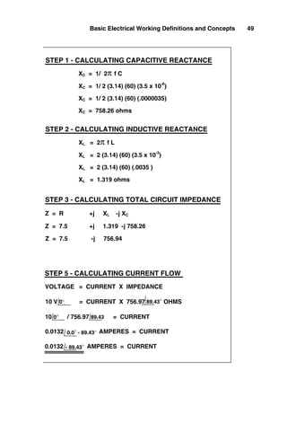
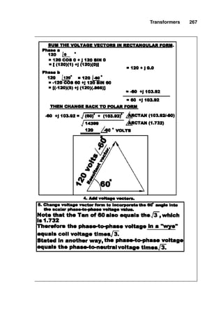
THEN
CHANGE
BACK
TO
POLAR
FORM
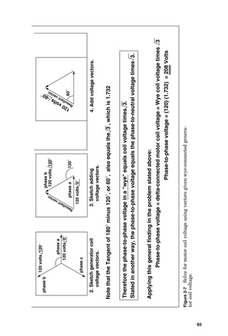
Making
a
diagram
of
the
circuit:
1.
Diagram
the
system
under
analysis.
CALCULATE
THE
DIFFERENCE
BETWEEN
THE
VOLTAGE
VECTORS
IN
RECTANGULAR
FORM.
=
43199
=
208
-150
°
TOTAL
VOLTS
64](https://image.slidesharecdn.com/libro-electricalcalculationhandbook-220531173735-cc042810/85/LIBRO-Electrical-Calculation-HandBook-pdf-89-320.jpg)

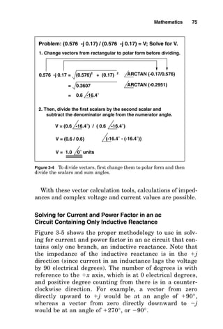
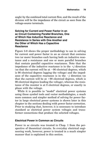
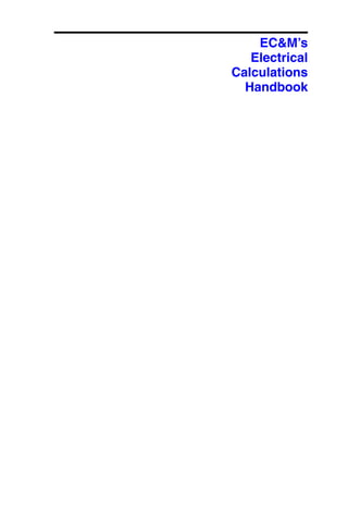
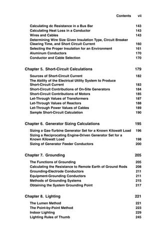
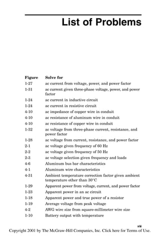
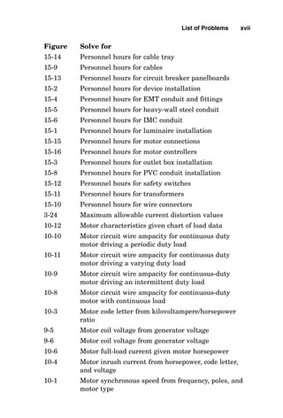
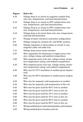
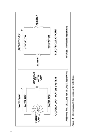
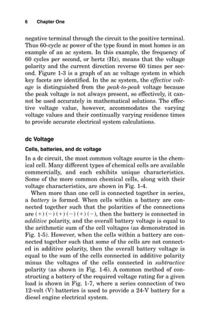
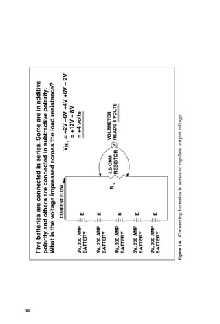
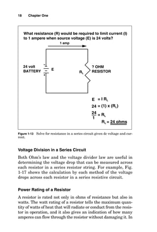
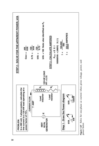
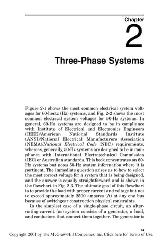
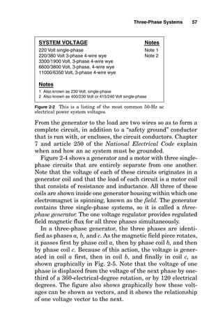
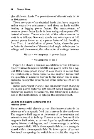
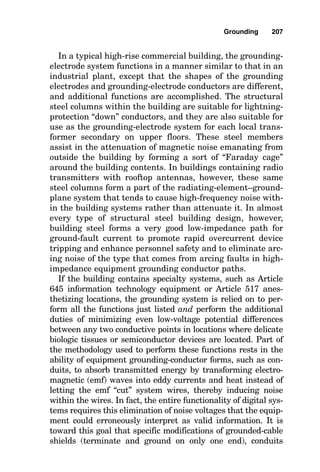
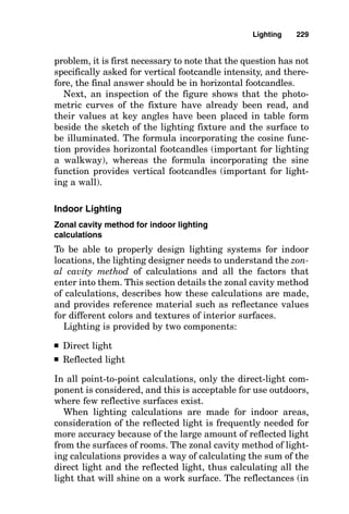
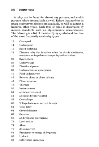
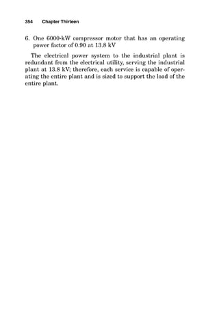
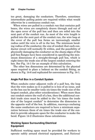
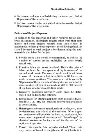
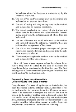
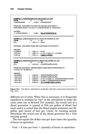
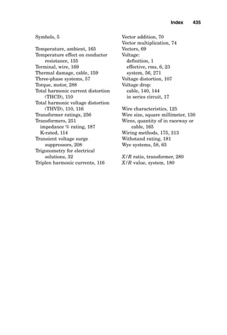
![VOLTAGE = CURRENT X IMPEDANCE
0.96 AMPERES = CURRENT
120 = CURRENT X 125 OHMS
120 / 125 = CURRENT
0°
0.0°- 53.1°
53.1°
0° 53.1°
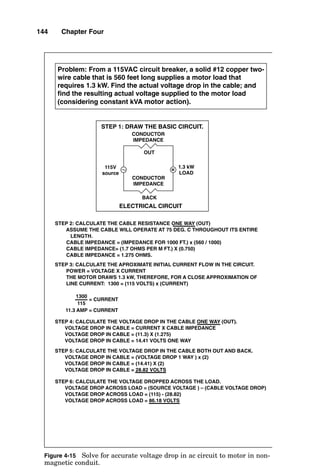
STEP 6 - CALCULATING CURRENT FLOW IN BRANCH A
0.96 AMPERES = CURRENT
- 53.1°
0.6 AMPERES = CURRENT
0.6 AMPERES = CURRENT
0.0° - (-90)°
120 / 200 = CURRENT
120 = CURRENT X 200 OHMS
STEP 7 - CALCULATING CURRENT FLOW IN BRANCH B
VOLTAGE = CURRENT X IMPEDANCE
0°
0° -90°
-90°
STEP 8 - SUM THE CURRENTS FROM BOTH BRANCHES
0.6 90°
= .6 COS 90 +j 0.6SIN 90
= [(.6)(0) +j (0.6)(1)]
= 0.576 -j 0.77
90°
= 0 +j 0.6
= 0.576 -j 0.17
BRANCH A
0.96 - 53.1°
= .96 COS 53.1 -j .96 SIN 53.1
= [ (0.96)(0.6) -j (0.96)(0.7996)
BRANCH B
0.576 -j 0.17 = (0.576)
2
+ (0.17)2
ARCTAN (0.17/0.576)
ARCTAN (0.2951)
0.3306
0.6 16.4° TOTAL AMPERES
STEP 10 - SOLVE FOR OVERALL IMPEDANCE
E = I X Z
120 = 0.6 X Z
0° 16.4°
120 / 0.6 = Z
0° 16.4°
200 = Z
0°-16.4°
200 OHMS = ZT
16.4°
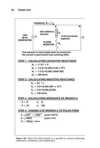
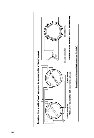
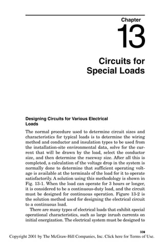
STEP 9 - SOLVE FOR POWER FACTOR.
POWER FACTOR = COS 16.4°
POWER FACTOR = .9593
83](https://image.slidesharecdn.com/libro-electricalcalculationhandbook-220531173735-cc042810/85/LIBRO-Electrical-Calculation-HandBook-pdf-108-320.jpg)
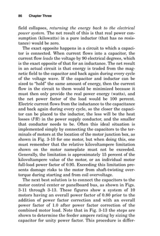
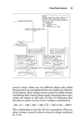
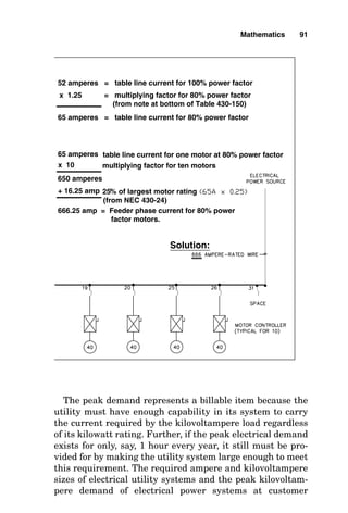
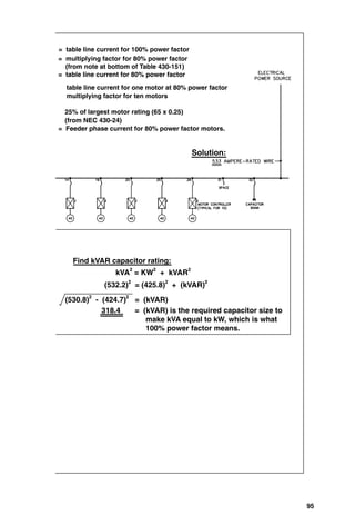
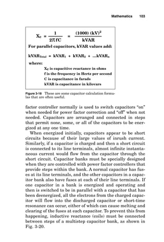
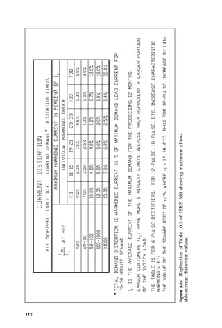
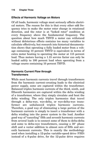
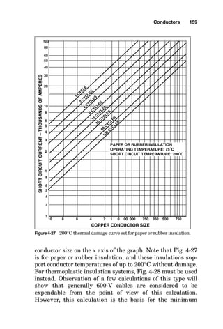
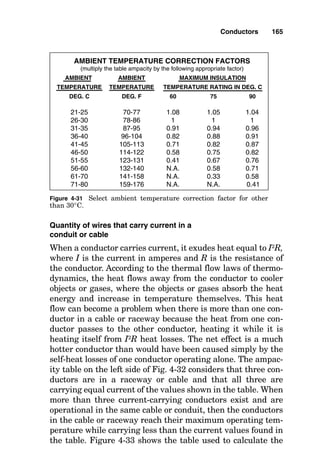
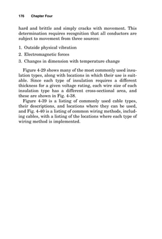
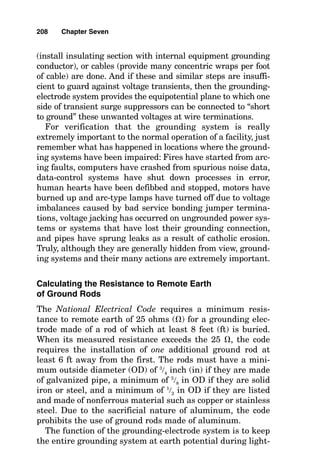
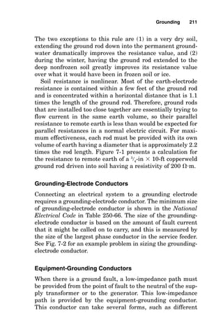
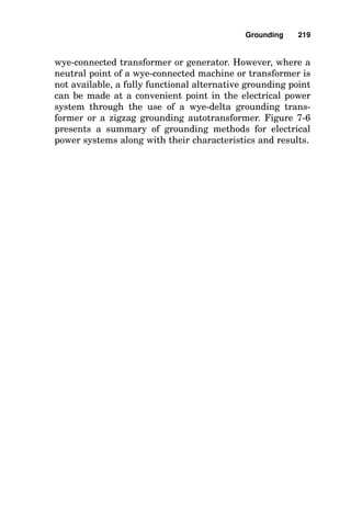
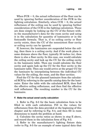
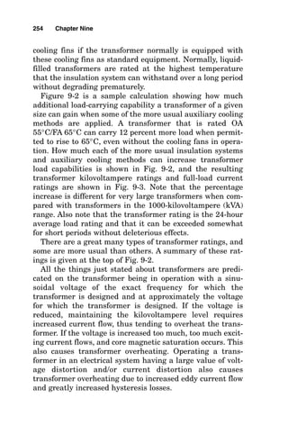
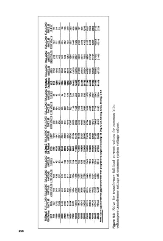
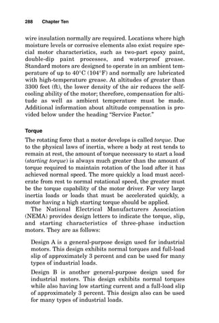
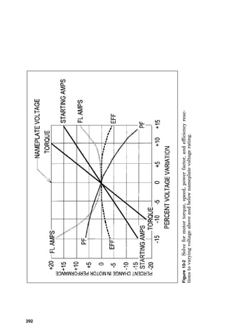
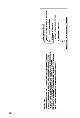
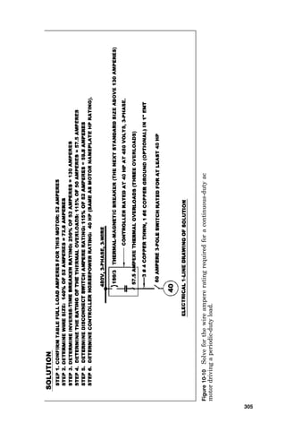
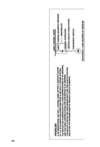
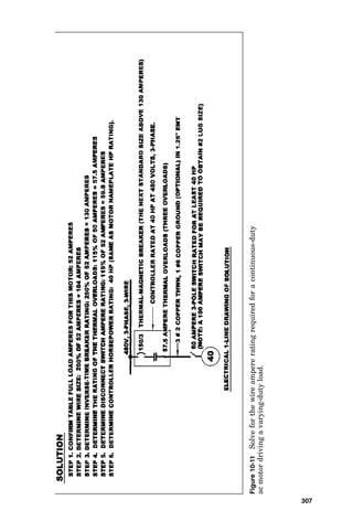
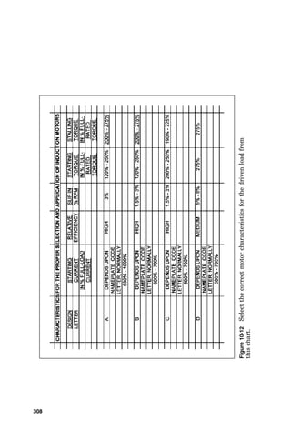
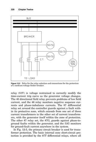
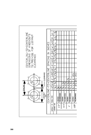
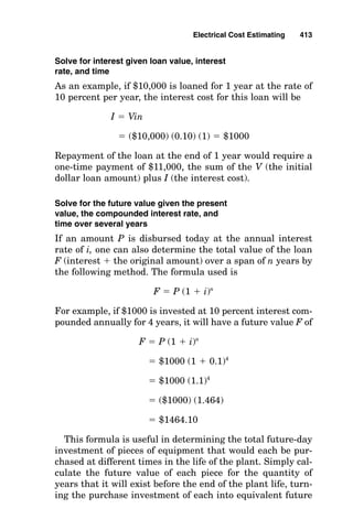
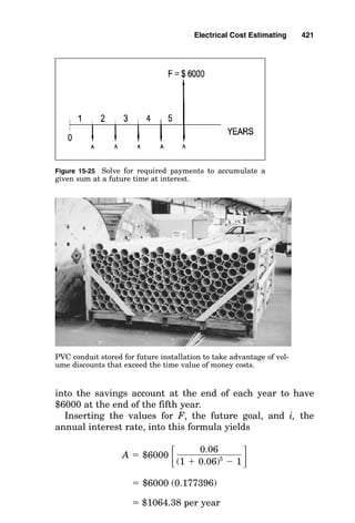
![ent from that followed in Fig. 3-12, where the factor of
1.25 [i.e., the multiplying factor from the bottom of
National Electrical Code (NEC) Table 430-151 for an indi-
vidual motor operating at 80 percent power factor] was not
used because power factor was corrected at each motor
(i.e., the branch-circuit current to each motor is as if the
motor is a 100 percent power factor load; therefore, the
note requiring this 1.25 factor at the bottom of NEC Table
430-151 was not applicable). In summary, power factor
can be corrected at each motor or at the motor control cen-
ter. There are benefits to correcting power factor at load
centers, including being able to correct beyond 95 percent
without causing motor problems and including a lowered
cost per reactive kilovoltampere when larger capacitor
units are installed.
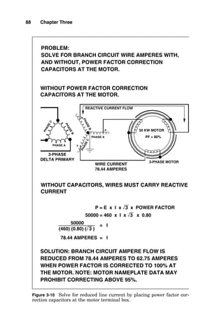
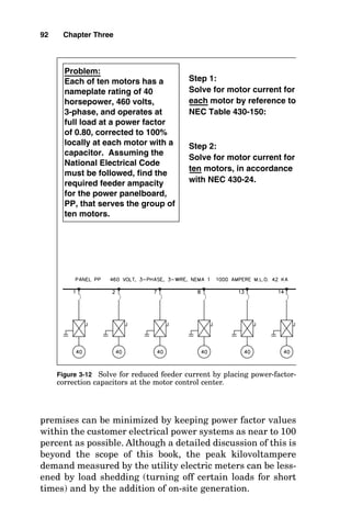
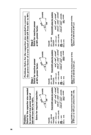
Power Factor Correction to Normal Limits
If an existing electrical system has become increasingly
loaded over time and its conductors are operating at their
maximum operating limit, often it is possible to permit
additional load simply by installing capacitors so that the
out-of-phase (lagging) current does not have to come from
the utility power source but instead can come from capac-
itors that are connected near the load. Figure 3-13 shows
how this application is made.
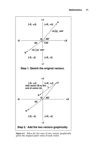
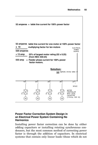
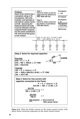
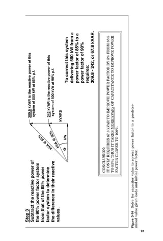
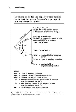
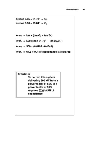
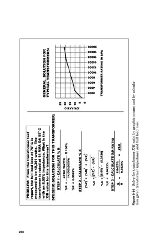
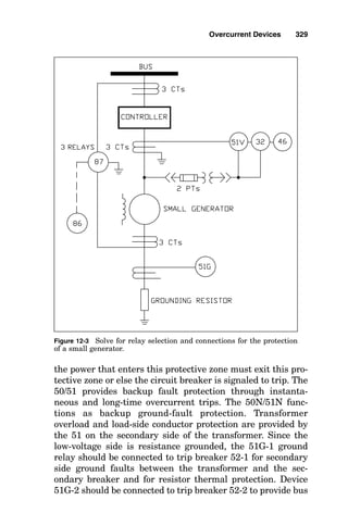
A review of the power triangle shown in Fig. 3-14 shows
that it takes much more capacitance to improve from a pow-
er factor of 0.95 to 1.0 than it takes to improve from a power
factor of 0.85 to 0.90. Since capacitors cost money, the amount
of capacitance that should be added to improve the power fac-
tor of the system generally is dictated by consideration of the
variables in the utility bill or by current-limitation consider-
ations in the supply conductor. Frequently, it is desirable to
change the power factor from some lagging value to an
improved value, but not quite to 1.0. Figure 3-15 shows a
quick method of calculating the amount of capacitance
required to change from an existing measured power factor to
an improved one.
Mathematics 87](https://image.slidesharecdn.com/libro-electricalcalculationhandbook-220531173735-cc042810/85/LIBRO-Electrical-Calculation-HandBook-pdf-112-320.jpg)
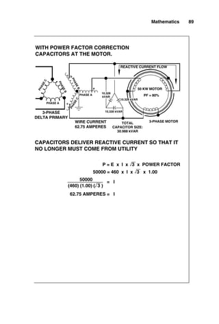
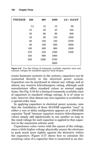
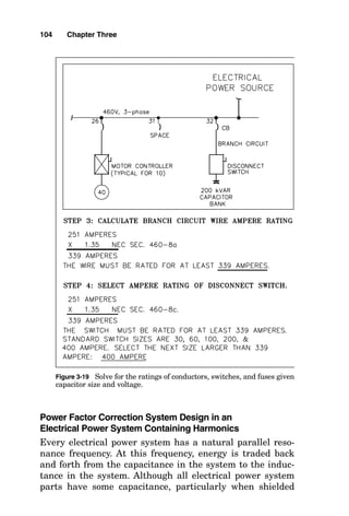
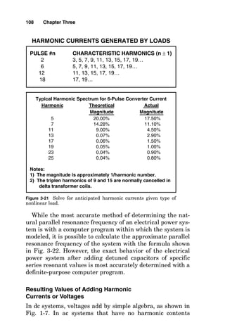
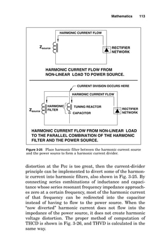
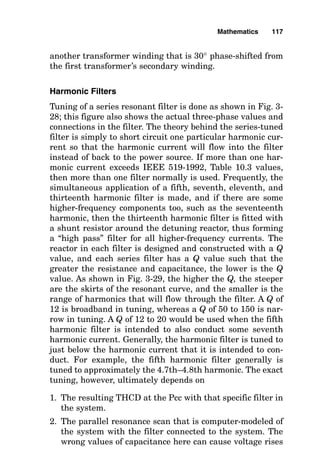
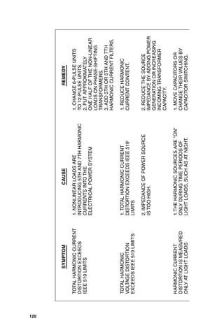
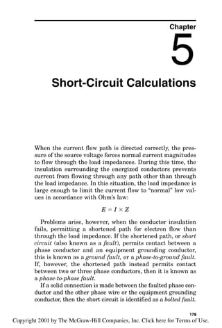
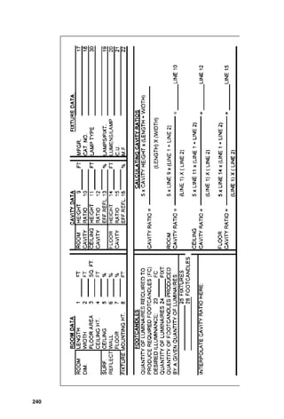
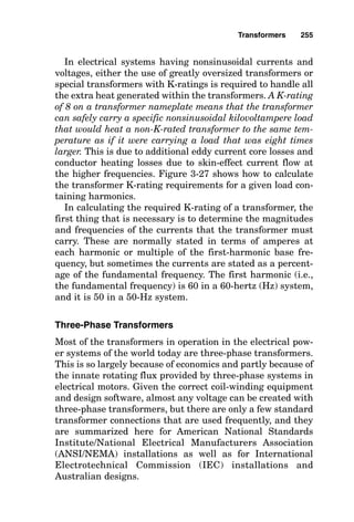
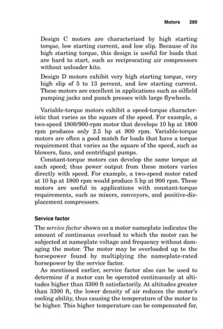
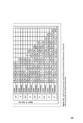
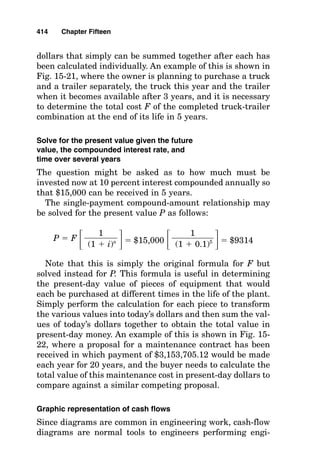
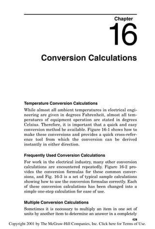
![correction capacitors, the natural parallel resonance fre-
quency of the electrical power system is reduced. At 100
percent power factor, the natural parallel resonance fre-
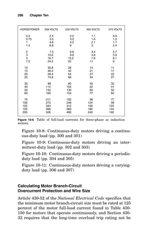
quency of an electrical power system can be expected to be
approximately at the fifth harmonic [i.e., if the frequency of
the system is 60 hertz (Hz), then the fifth harmonic is 5
times 60, or 300 Hz].
The natural resonance frequency of a system is of little
importance as long as only 60-Hz voltages and currents are
present in the electrical power system, since the system
capacitance and inductance will not begin to trade power
back and forth, or oscillate, unless the oscillation is initi-
ated by a harmonic source elsewhere in the electrical pow-
er system. Engineers can either field measure the
harmonic contents of an electrical power system or can
observe or computer model the system to determine
whether harmonic currents will exist there and what the
frequencies of those harmonic currents will be. Some
guidelines to forecasting the harmonic currents in an elec-
trical power system are shown in Fig. 3-21. This figure
shows the harmonic currents that are generated by certain
nonlinear loads, from which the harmonic currents flow
back to the electrical power source. In flowing back into the
source impedance of the electrical power source, the har-
monic currents create (Iharmonic Zsource) harmonic voltages
that “ride” on top of the fundamental 60-Hz sinusoidal
waveform, creating “voltage distortion.”
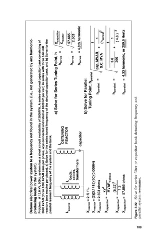
Calculating the Parallel Harmonic Resonance
of an Electrical Power System Containing
Capacitors
When the addition of capacitors is calculated to create a par-
allel harmonic resonance at a frequency that exists or is
forecast to exist in an electrical system, then reactors can be
added in series with the capacitors to “detune” the capacitor
bank from the specific parallel resonance frequency to
another frequency that does not exist in the system.
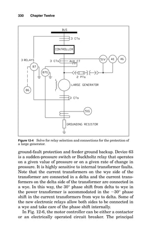
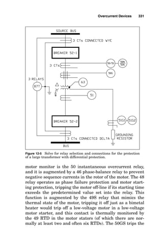
Mathematics 107](https://image.slidesharecdn.com/libro-electricalcalculationhandbook-220531173735-cc042810/85/LIBRO-Electrical-Calculation-HandBook-pdf-132-320.jpg)


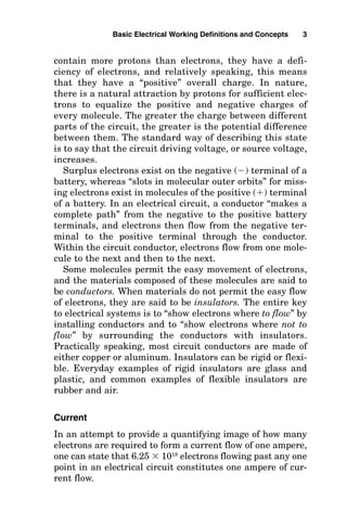
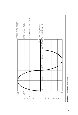
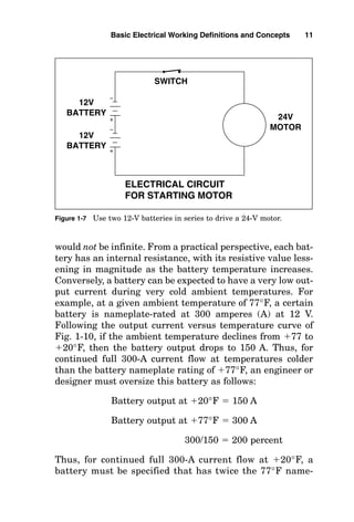
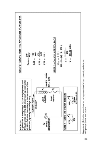
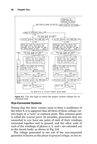
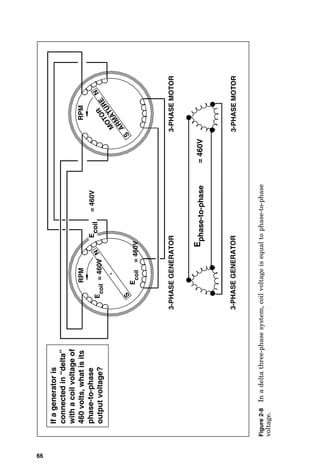
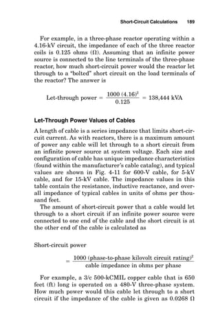
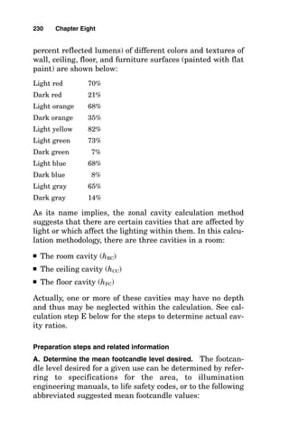
![ELECTRICAL
CIRCUIT
LOAD
CONDUCTOR
IMPEDANCE
CONDUCTOR
IMPEDANCE
Phase
A
208V
3-phase
source
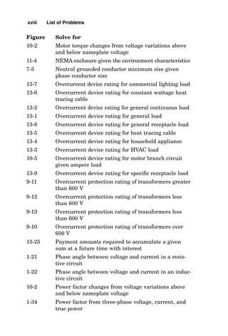
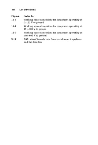
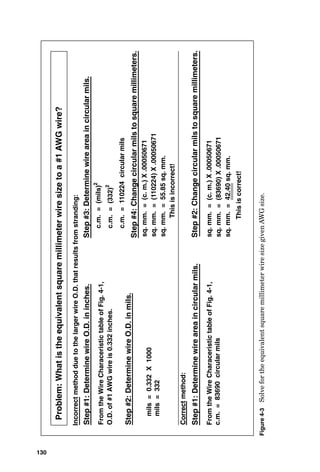
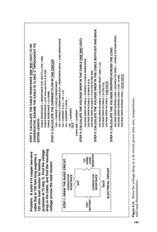
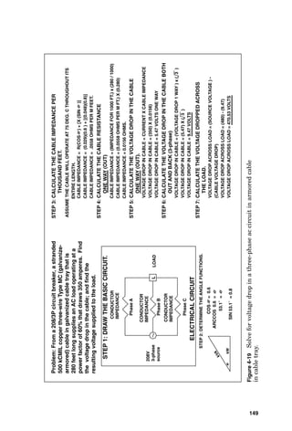
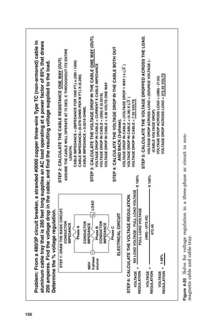
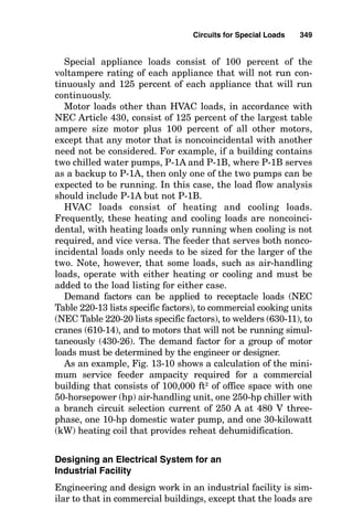
Problem:
From
a
208/3P
circuit
breaker,
a
stranded
500
kCMIL
copper
three-wire
Type
MC
(galvanize-
armored)
cable
in
galvanized
cable
tray
that
is
280
feet
long
supplies
an
AC
load
operating
at
a
power
factor
of
60%
that
draws
350
amperes.
Find
the
voltage
drop
in
the
cable;
and
find
the
resulting
voltage
supplied
to
the
load.
STEP
1:
DRAW
THE
BASIC
CIRCUIT.
L
CONDUCTOR
IMPEDANCE
Phase
B
Phase
C
STEP
2:
DETERMINE
THE
ANGLE
FUNCTIONS.
COS
=
0.6
ARCCOS
0.6
=
53.1
°
=
SIN
53.1
°
=
0.8
kW
k
V
A
STEP
4:
CALCULATE
THE
CABLE
RESISTANCE
ONE
WAY
(OUT)
CABLE
IMPEDANCE
=
(IMPEDANCE
FOR
1000
FT.)
x
(280
/
1000)
CABLE
IMPEDANCE
=
(0.0558
OHMS
PER
M
FT.)
X
(0.280)
CABLE
IMPEDANCE
=
0.0156
OHMS.
VOLTAGE
DROP
IN
CABLE
=
CURRENT
X
CABLE
IMPEDANCE
VOLTAGE
DROP
IN
CABLE
=
(350)
X
(0.0156)
VOLTAGE
DROP
IN
CABLE
=
5.47
VOLTS
ONE
WAY
STEP
5:
CALCULATE
THE
VOLTAGE
DROP
IN
THE
CABLE
ONE
WAY
(OUT).
STEP
6:
CALCULATE
THE
VOLTAGE
DROP
IN
THE
CABLE
BOTH
OUT
AND
BACK
(3-phase)
VOLTAGE
DROP
IN
CABLE
=
(VOLTAGE
DROP
1
WAY
)
x
(
3
)
VOLTAGE
DROP
IN
CABLE
=
(5.47)
X
(
3
)
VOLTAGE
DROP
IN
CABLE
=
9.47
VOLTS
STEP
7:
CALCULATE
THE
VOLTAGE
DROPPED
ACROSS
THE
LOAD.
VOLTAGE
DROP
ACROSS
LOAD
=
(SOURCE
VOLTAGE
)
-
(CABLE
VOLTAGE
DROP)
VOLTAGE
DROP
ACROSS
LOAD
=
(480)
-
(9.47)
VOLTAGE
DROP
ACROSS
LOAD
=
470.53
VOLTS
STEP
3:
CALCULATE
THE
CABLE
IMPEDANCE
PER
THOUSAND
FEET.
ASSUME
THE
CABLE
WILL
OPERATE
AT
75
DEG.
C
THROUGHOUT
ITS
ENTIRE
LENGTH.
CABLE
IMPEDANCE
=
R(COS
)
+
[X
(SIN
)]
CABLE
IMPEDANCE
=
(0.029)(0.6
)
+
[(0.048)(0.8)]
CABLE
IMPEDANCE
=
.0558
OHMS
PER
M
FEET.
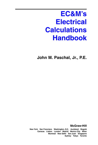
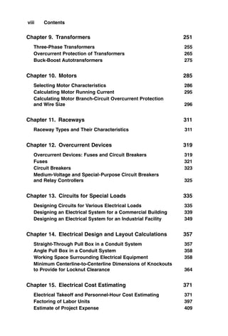
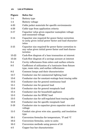
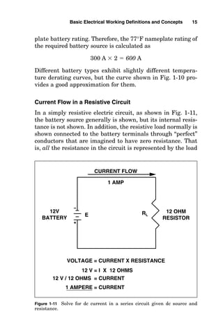
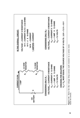
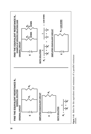
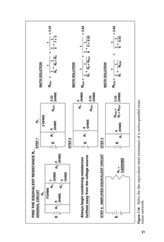
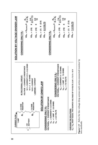
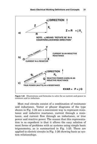
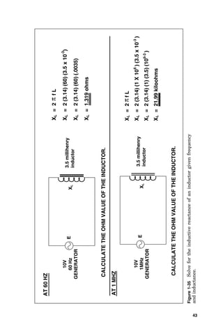
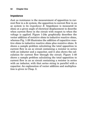
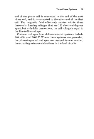
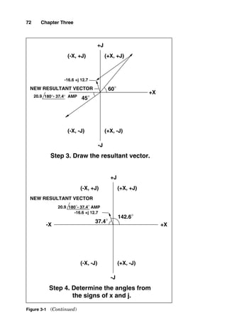
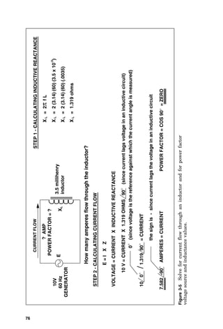
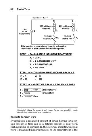
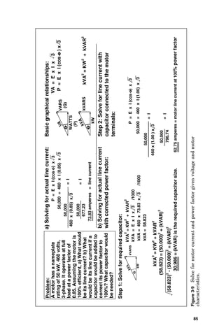
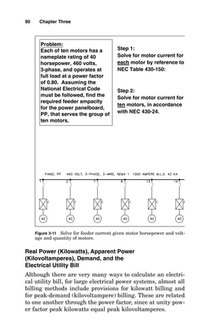
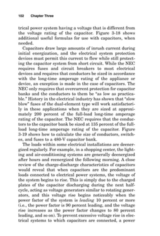
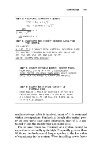
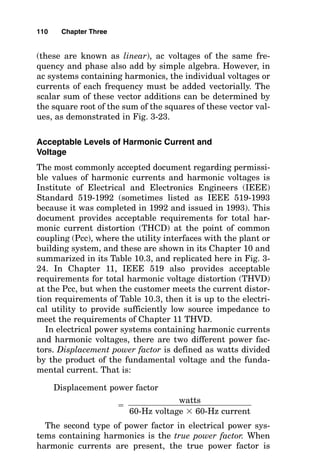
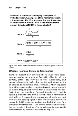
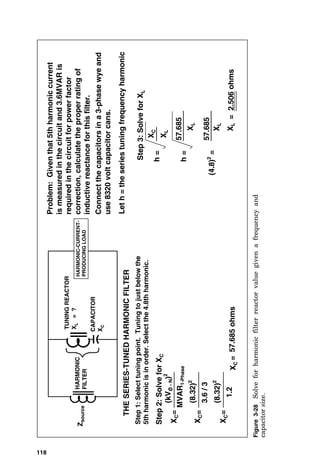
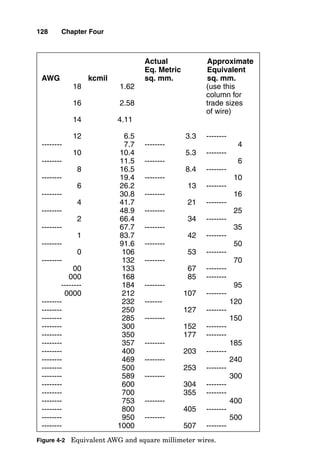
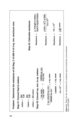
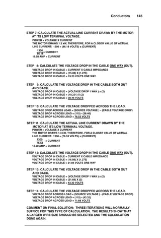
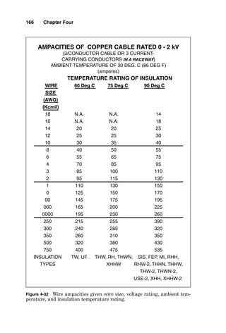
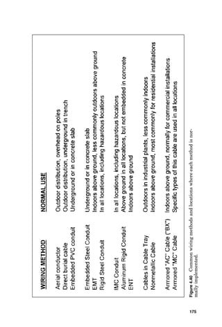
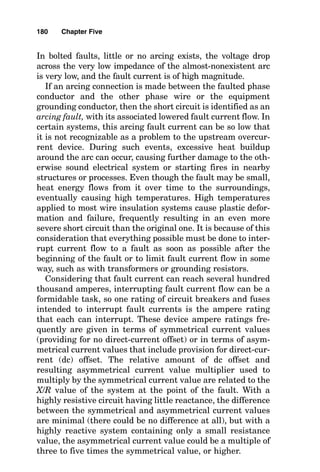
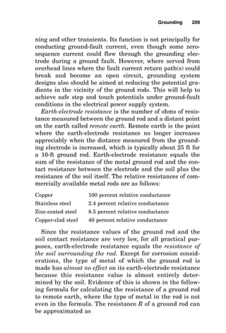
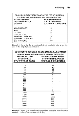
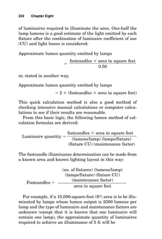
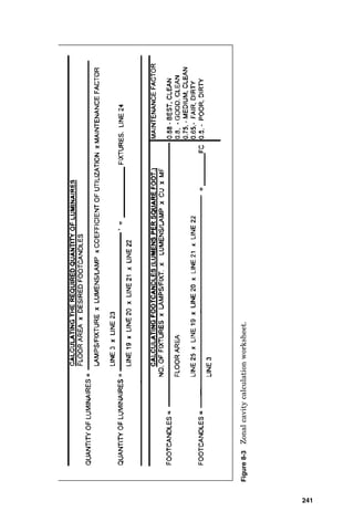
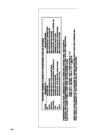
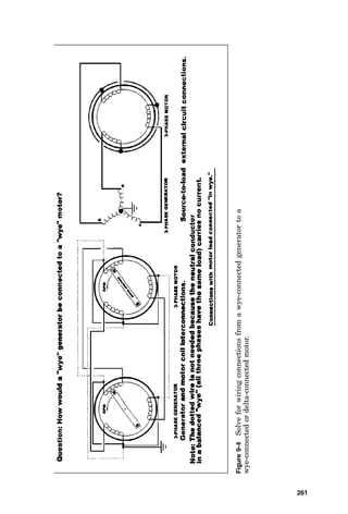
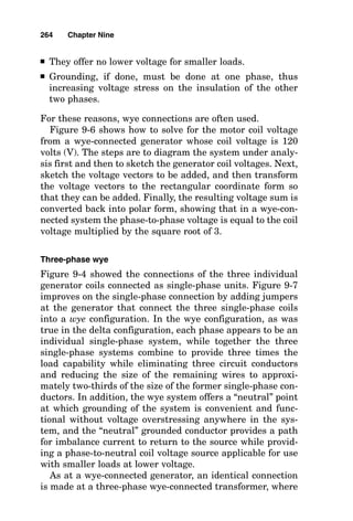
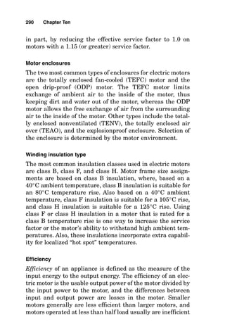
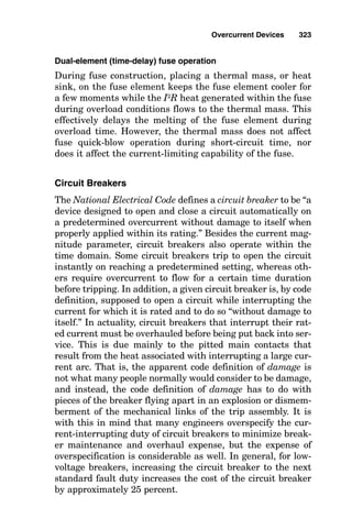
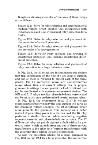
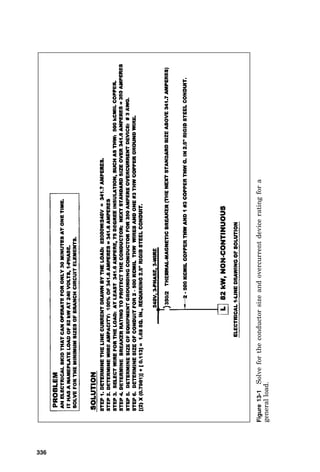
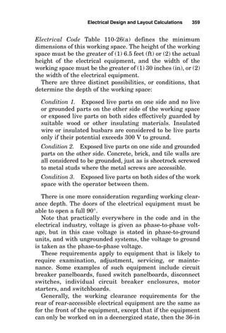
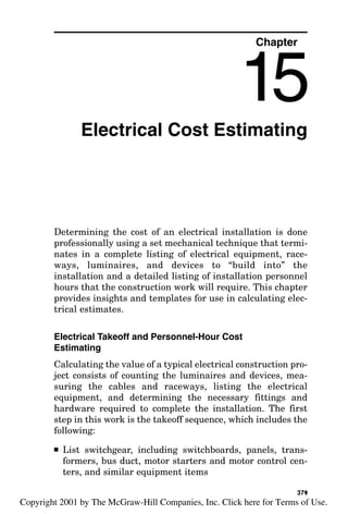
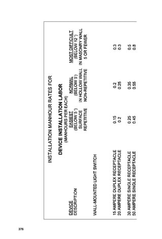
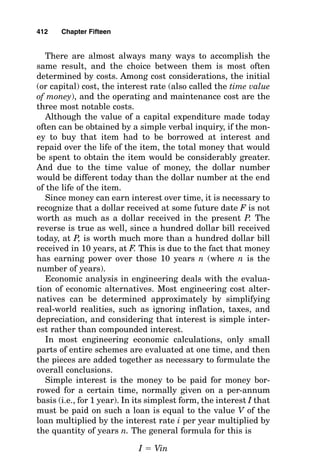
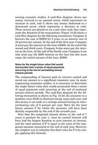
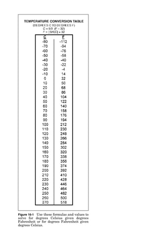
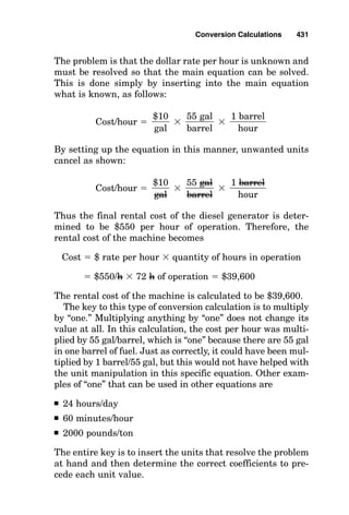
Figure
4-19
Solve
for
voltage
drop
in
a
three-phase
ac
circuit
in
armored
cable
in
cable
tray.
149](https://image.slidesharecdn.com/libro-electricalcalculationhandbook-220531173735-cc042810/85/LIBRO-Electrical-Calculation-HandBook-pdf-176-320.jpg)
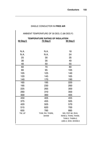
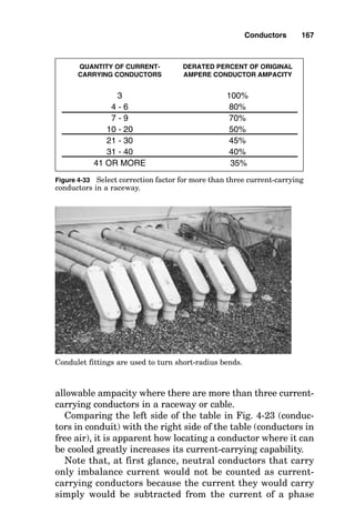
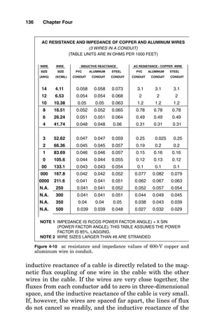
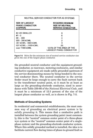
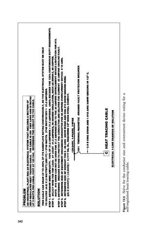
![conductor in the cable or raceway, and this would be true if
the conductors all carried only fundamental current (60 Hz).
If the load served by the conductors generates third harmon-
ic current, such as does arc-type lighting, the third harmonic
is present in the neutral conductor from each of the three
phases. The net effect of this is that the neutral conductor
heats at almost the same rate as do the phase conductors,
and so the neutral conductor must be counted as a current-
carrying conductor.
Location where the heat cannot escape from
the cable very rapidly
In the thermal flow equation, British thermal units (Btus) of
heat must flow from the operating conductor through thermal
resistance. If the thermal resistance is very high, then the
heat cannot flow away, and the operating conductor increases
in temperature. Consider the case of a cable that is either
buried in the earth or is pulled into a conduit that is buried in
the earth. Some forms of earth carry heat very well, and oth-
ers are essentially thermal insulators. Heat flows from buried
cables through the earth and to the air above the earth. The
actual computer modeling to determine the ultimate allow-
able line current for a cable or cables buried underground is
beyond the scope of this book, but suffice it to state that the
Neher-McGrath method [American Institute of Electrical
Engineers (AIEE) Paper 57-660] of ampacity calculation
should be referred to when a cable is buried deeper than 36
inches (in) or when more than one cable is installed near
another.
Location where the heat can escape from
the cable very rapidly
When a continuous supply of cool air is available to flow
over a conductor, then thermal flow can occur continuously
to maintain a cool conductor temperature, even when the
conductor is carrying current. Thermal flow is improved so
much when a single insulated conductor is located in “free
air” that it takes a great deal more current to elevate the
conductor to its maximum operating temperature.
168 Chapter Four](https://image.slidesharecdn.com/libro-electricalcalculationhandbook-220531173735-cc042810/85/LIBRO-Electrical-Calculation-HandBook-pdf-195-320.jpg)


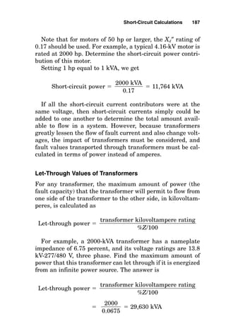
![Generally, this value can be gotten from the electrical utili-
ty company by a simple request and is most often given in
amperes or kilovoltamperes.
Suppose that the utility company electrical system inter-
face data are given as
MVASC 2500 at 138 kilovolts (kV) with an X/R
7 at the interface point
For this system, the utility can deliver 2,500,000 kilo-
voltamperes (kVA) ÷ [138 kV(兹3
苶)], or a total of 10,459 sym-
metrical amperes (A) of short-circuit current.
The short-circuit value from the electrical utility company
will be “added to” by virtue of contributions from the on-site
generator and motor loads within the plant or building elec-
trical power system. That is, the short-circuit value at the
interface point with the electrical utility will be greater than
just the value of the utility contribution alone.
Short-Circuit Contributions of On-Site
Generators
The nameplate of each on-site generator is marked with its
subtransient reactance Xd″ like this. This subtransient val-
ue occurs immediately after a short circuit and only contin-
ues for a few cycles. For short-circuit current calculations,
the subtransient reactance value is used because it produces
the most short-circuit current.
Determining how many kilovoltamperes an on-site genera-
tor can contribute to the short-circuit current of an electrical
power system is a simple one-step process, solved as follows:
Short-circuit kVA
For example, a typical synchronous generator connected to
a 5000 shaft horsepower (shp) gas turbine engine is rated at
7265 kVA, and its subtransient reactance Xd″ is 0.17. The
generator kVA rating
Xd″ rating
184 Chapter Five](https://image.slidesharecdn.com/libro-electricalcalculationhandbook-220531173735-cc042810/85/LIBRO-Electrical-Calculation-HandBook-pdf-211-320.jpg)
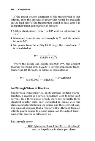

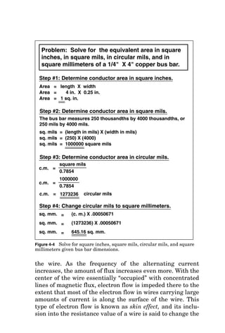
![tem voltage at the terminals of the motor being started and
around 90 percent of the normal system voltage at the genera-
tor switchgear bus. A good rule of thumb to achieve this is to
assume that the generator has a subtransient reactance of
approximately 15 percent (normally this is a valid assumption)
and then to select a generator set whose kilowatt rating
exceeds the total kilowattage of the summed loads [setting 1
kilowatt (kW) equal to 1 horsepower (hp) for this calculation]
and whose kilovoltampere rating is equal to or greater than 50
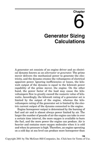
Generator Sizing Calculations 199
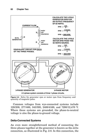
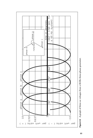
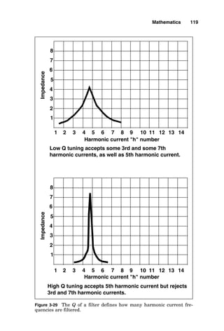
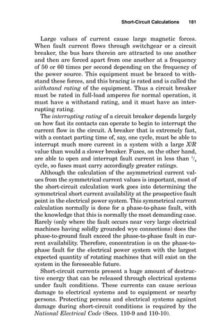
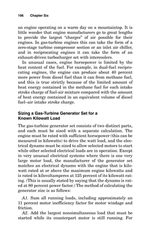
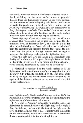
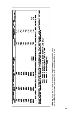
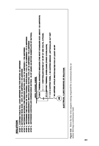
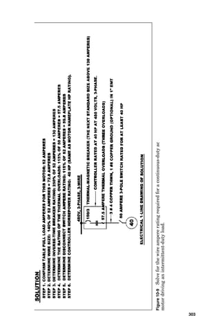
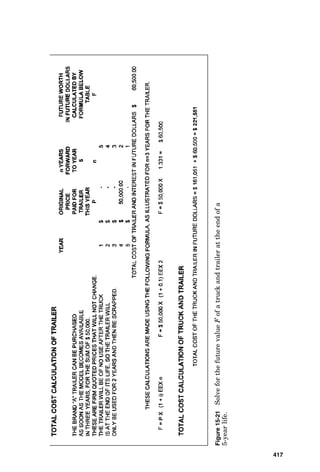
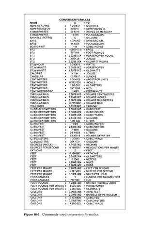
Figure 6-1 Solve for generator site rating given load, temperature, and
altitude.](https://image.slidesharecdn.com/libro-electricalcalculationhandbook-220531173735-cc042810/85/LIBRO-Electrical-Calculation-HandBook-pdf-226-320.jpg)
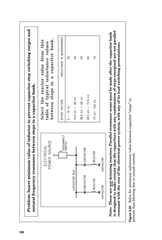
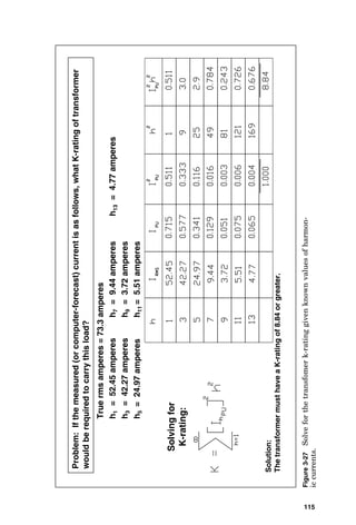
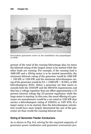
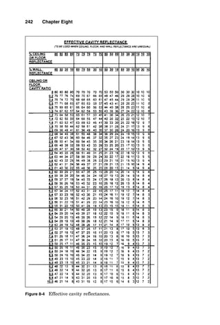
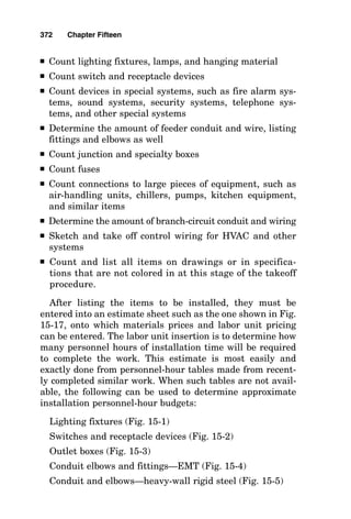
![percent of the total of the running kilowattage plus six times
the kilowatt rating of the largest motor to be started while the
other loads are running. For example, if the running load is
1000 kW and a 150-hp motor is to be started meanwhile, the
minimum kilowatt rating of the generator would be 1000 kW
150 kW, or 1150 kW, and the minimum kilovoltampere rat-
ing of the generator would be 0.5 [1000 kW 6(150)], or 950
kilovoltamperes (kVA). Select a generator set that meets or
exceeds both the 1150-kW and the 950-kVA requirements and
that has a voltage regulator that can offset approximately a 15
percent internal voltage dip (15 percent regulation) while the
large motor is starting. In this case, the usual offering of a gen-
erator set manufacturer would be a set rated at 1150 kW that
carries a kilovoltampere rating of 1150/0.8, or 1437 kVA. If a
larger motor is to be started, then the kilovoltampere calcula-
tion would have more largely determined the size of the gen-
erator set than would the running kilowatt load.
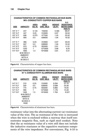
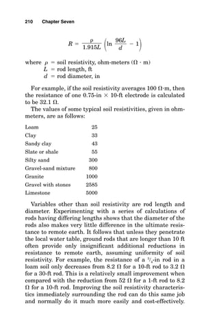
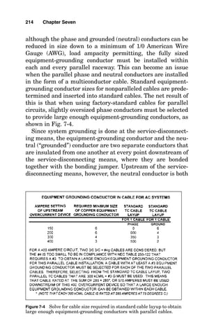
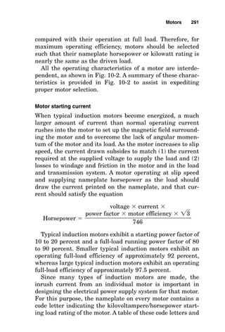
Sizing of Generator Feeder Conductors
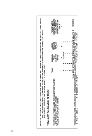
As is shown in Fig. 6-2, solving for the required ampacity of
generator power conductors and generator overcurrent pro-
200 Chapter Six
Gas-turbine generators arrive at the installation site prepackaged
on skids.](https://image.slidesharecdn.com/libro-electricalcalculationhandbook-220531173735-cc042810/85/LIBRO-Electrical-Calculation-HandBook-pdf-227-320.jpg)


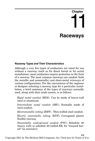
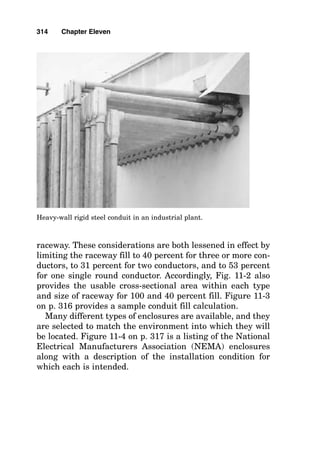
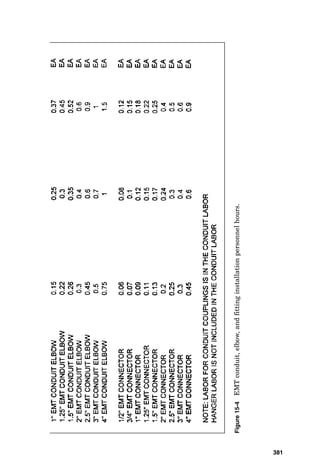
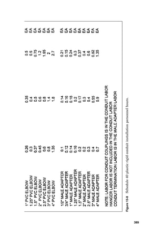
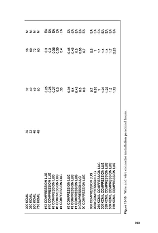
![Raceways
Raceway Types and Their Characteristics
Although a very few types of conductors are rated for use
without a raceway (such as for direct burial or for aerial
installation), most conductors require protection in the form
of a raceway. The most common raceways are conduit (both
the metallic and nonmetallic) and sheet-metal wireways of
various configurations. For the convenience of the engineer
or designer selecting a raceway type for a particular instal-
lation, a brief summary of the types of raceways normally
used, along with their trade names, is as follows:
Rigid metal conduit (RGS). Can be made of heavy-wall
steel or aluminum.
Intermediate metal conduit (IMC). Normally made of
steel conduit.
Electrometallic tubing (EMT). Thin-walled steel conduit.
Electric nonmetallic tubing (ENT). Corrugated plastic
flexible raceway.
Nonmetallic underground conduit (PVC). Schedule 40
(heavy wall) or schedule 20 [called EB, for “encased bur-
ial” (in concrete)].
Chapter
11
311
v
Copyright 2001 by The McGraw-Hill Companies, Inc. Click here for Terms of Use.](https://image.slidesharecdn.com/libro-electricalcalculationhandbook-220531173735-cc042810/85/LIBRO-Electrical-Calculation-HandBook-pdf-340-320.jpg)


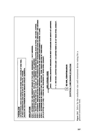
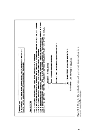
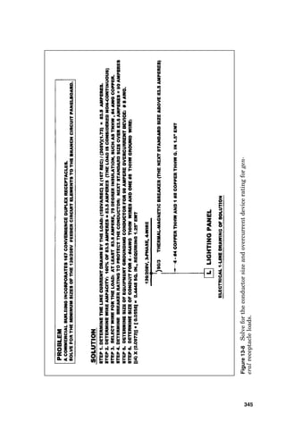
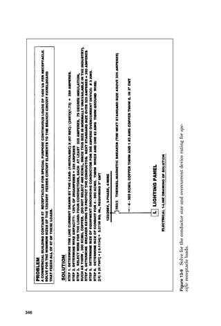
![to the National Electrical Code (NEC), which now sets the
standards for the characteristics of the required electrical
system. Accordingly, this book both points out the require-
ments using calculation methodology and provides NEC ref-
erence information where the engineer and designer can
obtain further information.
For every feeder and switchgear bus, panelboard bus, or
motor control center bus, a separate calculation must be
made; however, these calculations are all very similar, with
only the connected loads changing. The first of the calcula-
tions that must be made is for the service feeder and service
equipment.
The following six general groups of loads must be consid-
ered within commercial buildings:
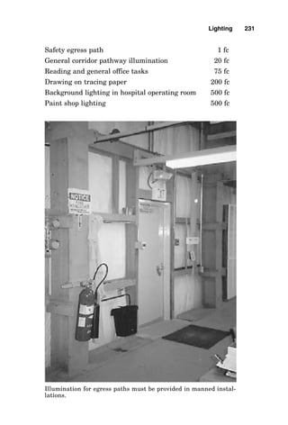
1. Lighting
2. Receptacle loads
3. Special appliance loads
4. Motor loads other than heating, ventilation, and air-con-
ditioning (HVAC) loads
5. The greater of
a. HVAC compressor loads and hermetically sealed
motor loads, or
b. Heating loads
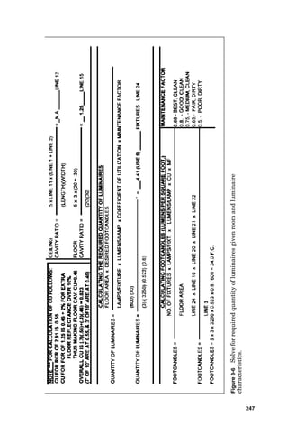
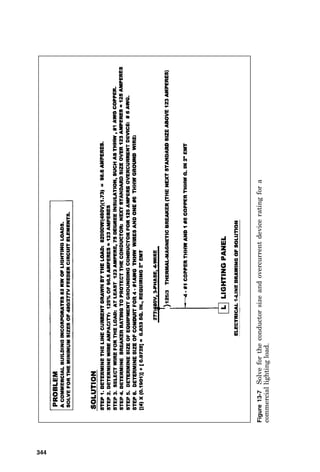
Lighting loads consist of
1. The greater of 125 percent (for continuous operation) of
the quantity of voltamperes per square foot shown in
NEC Table 220-3(a) or 125 percent of the actual lighting
fixture load, including low-voltage lighting (Article 411),
outdoor lighting, and 1200-voltampere (VA) sign circuit
[600-4(b)(3)].
2. 125 percent of show window lighting [220-12(a)].
3. Track lighting at 125 percent of 150 VA per lineal foot
[220-12(b)].
Receptacle loads consist of
1. 100 percent of the quantity of 1 VA/ft2 shown in Table 220-
3(a) or 100 percent of 180 VA per receptacle [220-3(b)(9)].
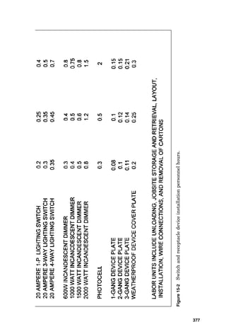
Circuits for Special Loads 347](https://image.slidesharecdn.com/libro-electricalcalculationhandbook-220531173735-cc042810/85/LIBRO-Electrical-Calculation-HandBook-pdf-376-320.jpg)


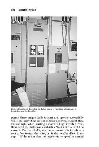
![UNIT-I Final (1)[1].pptfgcvhvjgbjhbjgbjhhvhvhvh](https://cdn.slidesharecdn.com/ss_thumbnails/unit-ifinal11-251129122433-e786871d-thumbnail.jpg?width=640&height=640&fit=bounds)


![[Deck] What's New in Spark-Iceberg Integration via DSV2.pptx](https://cdn.slidesharecdn.com/ss_thumbnails/deckwhatsnewinspark-icebergintegrationviadsv2-260210005337-25955b12-thumbnail.jpg?width=640&height=640&fit=bounds)


