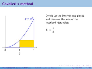
Download as PDF, PPTX

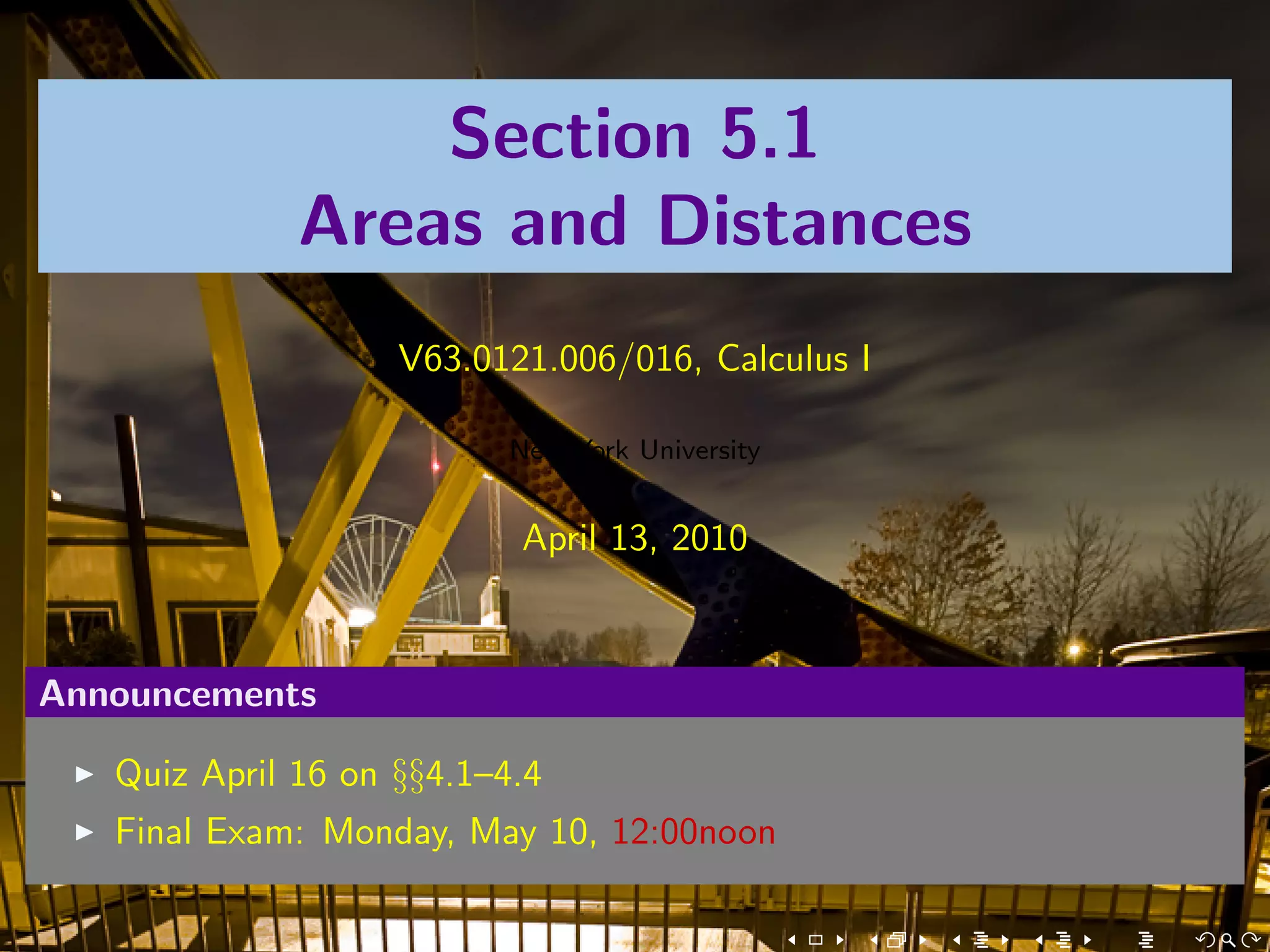

![What is Ln ?
1
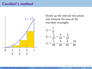
Divide the interval [0, 1] into n pieces. Then each has width .
n
V63.0121.006/016, Calculus I (NYU) Section 5.1 Areas and Distances April 13, 2010 15 / 30](https://image.slidesharecdn.com/lesson22-areasanddistancesslides-100413152044-phpapp02/85/Lesson-22-Areas-and-Distances-38-320.jpg)
![What is Ln ?
1
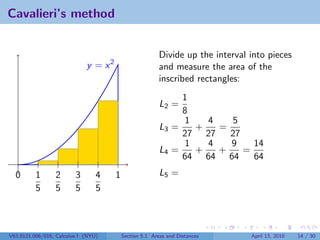
Divide the interval [0, 1] into n pieces. Then each has width . The
n
rectangle over the ith interval and under the parabola has area
2
1 i −1 (i − 1)2
· = .
n n n3
V63.0121.006/016, Calculus I (NYU) Section 5.1 Areas and Distances April 13, 2010 15 / 30](https://image.slidesharecdn.com/lesson22-areasanddistancesslides-100413152044-phpapp02/85/Lesson-22-Areas-and-Distances-39-320.jpg)
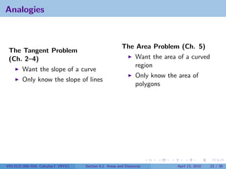
![What is Ln ?
1
Divide the interval [0, 1] into n pieces. Then each has width . The
n
rectangle over the ith interval and under the parabola has area
2
1 i −1 (i − 1)2
· = .
n n n3
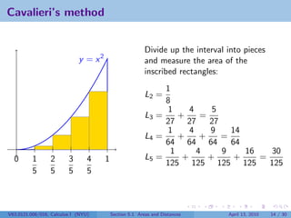
So
1 22 (n − 1)2 1 + 22 + 32 + · · · + (n − 1)2
Ln = + 3 + ··· + =
n3 n n3 n3
V63.0121.006/016, Calculus I (NYU) Section 5.1 Areas and Distances April 13, 2010 15 / 30](https://image.slidesharecdn.com/lesson22-areasanddistancesslides-100413152044-phpapp02/85/Lesson-22-Areas-and-Distances-40-320.jpg)
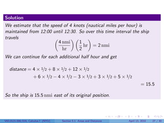
![What is Ln ?
1
Divide the interval [0, 1] into n pieces. Then each has width . The
n
rectangle over the ith interval and under the parabola has area
2
1 i −1 (i − 1)2
· = .
n n n3
So
1 22 (n − 1)2 1 + 22 + 32 + · · · + (n − 1)2
Ln = + 3 + ··· + =
n3 n n3 n3
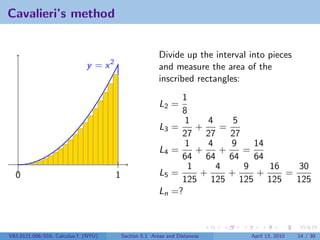
The Arabs knew that
n(n − 1)(2n − 1)
1 + 22 + 32 + · · · + (n − 1)2 =
6
So
n(n − 1)(2n − 1)
Ln =
6n3
V63.0121.006/016, Calculus I (NYU) Section 5.1 Areas and Distances April 13, 2010 15 / 30](https://image.slidesharecdn.com/lesson22-areasanddistancesslides-100413152044-phpapp02/85/Lesson-22-Areas-and-Distances-41-320.jpg)
![What is Ln ?
1
Divide the interval [0, 1] into n pieces. Then each has width . The
n
rectangle over the ith interval and under the parabola has area
2
1 i −1 (i − 1)2
· = .
n n n3
So
1 22 (n − 1)2 1 + 22 + 32 + · · · + (n − 1)2
Ln = + 3 + ··· + =
n3 n n3 n3
The Arabs knew that
n(n − 1)(2n − 1)
1 + 22 + 32 + · · · + (n − 1)2 =
6
So
n(n − 1)(2n − 1) 1
Ln = →
6n3 3
as n → ∞.
V63.0121.006/016, Calculus I (NYU) Section 5.1 Areas and Distances April 13, 2010 15 / 30](https://image.slidesharecdn.com/lesson22-areasanddistancesslides-100413152044-phpapp02/85/Lesson-22-Areas-and-Distances-42-320.jpg)
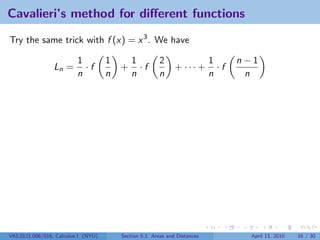
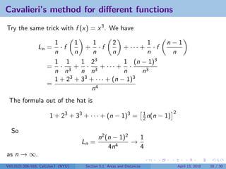

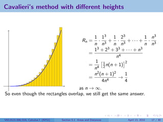
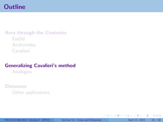
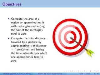
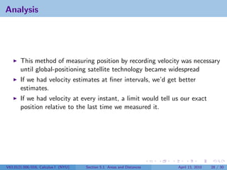
![Cavalieri’s method in general
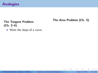
Let f be a positive function defined on the interval [a, b]. We want to find the area
between x = a, x = b, y = 0, and y = f (x).
b−a
For each positive integer n, divide up the interval into n pieces. Then ∆x = .
n
For each i between 1 and n, let xi be the nth step between a and b. So
x0 = a
b−a
x1 = x0 + ∆x = a +
n
b−a
x2 = x1 + ∆x = a + 2 ·
n
······
b−a
xi = a + i ·
n
······
a b b−a
x0 x1 x2 . . . xi xn−1xn xn = a + n · =b
n
V63.0121.006/016, Calculus I (NYU) Section 5.1 Areas and Distances April 13, 2010 19 / 30](https://image.slidesharecdn.com/lesson22-areasanddistancesslides-100413152044-phpapp02/85/Lesson-22-Areas-and-Distances-51-320.jpg)
![Cavalieri’s method in general
Let f be a positive function defined on the interval [a, b]. We want to find the area
between x = a, x = b, y = 0, and y = f (x).
b−a
For each positive integer n, divide up the interval into n pieces. Then ∆x = .
n
For each i between 1 and n, let xi be the nth step between a and b. So
x0 = a
b−a
x1 = x0 + ∆x = a +
n
b−a
x2 = x1 + ∆x = a + 2 ·
n
······
b−a
xi = a + i ·
n
······
a b b−a
x0 x1 x2 . . . xi xn−1xn xn = a + n · =b
n
V63.0121.006/016, Calculus I (NYU) Section 5.1 Areas and Distances April 13, 2010 19 / 30](https://image.slidesharecdn.com/lesson22-areasanddistancesslides-100413152044-phpapp02/85/Lesson-22-Areas-and-Distances-52-320.jpg)
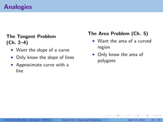
![Cavalieri’s method in general
Let f be a positive function defined on the interval [a, b]. We want to find the area
between x = a, x = b, y = 0, and y = f (x).
b−a
For each positive integer n, divide up the interval into n pieces. Then ∆x = .
n
For each i between 1 and n, let xi be the nth step between a and b. So
x0 = a
b−a
x1 = x0 + ∆x = a +
n
b−a
x2 = x1 + ∆x = a + 2 ·
n
······
b−a
xi = a + i ·
n
······
a b b−a
x0 x1 x2 . . . xi xn−1xn xn = a + n · =b
n
V63.0121.006/016, Calculus I (NYU) Section 5.1 Areas and Distances April 13, 2010 19 / 30](https://image.slidesharecdn.com/lesson22-areasanddistancesslides-100413152044-phpapp02/85/Lesson-22-Areas-and-Distances-53-320.jpg)
![Cavalieri’s method in general
Let f be a positive function defined on the interval [a, b]. We want to find the area
between x = a, x = b, y = 0, and y = f (x).
b−a
For each positive integer n, divide up the interval into n pieces. Then ∆x = .
n
For each i between 1 and n, let xi be the nth step between a and b. So
x0 = a
b−a
x1 = x0 + ∆x = a +
n
b−a
x2 = x1 + ∆x = a + 2 ·
n
······
b−a
xi = a + i ·
n
······
a b b−a
x0 x1 x2 . . . xi xn−1xn xn = a + n · =b
n
V63.0121.006/016, Calculus I (NYU) Section 5.1 Areas and Distances April 13, 2010 19 / 30](https://image.slidesharecdn.com/lesson22-areasanddistancesslides-100413152044-phpapp02/85/Lesson-22-Areas-and-Distances-54-320.jpg)
![Cavalieri’s method in general
Let f be a positive function defined on the interval [a, b]. We want to find the area
between x = a, x = b, y = 0, and y = f (x).
b−a
For each positive integer n, divide up the interval into n pieces. Then ∆x = .
n
For each i between 1 and n, let xi be the nth step between a and b. So
x0 = a
b−a
x1 = x0 + ∆x = a +
n
b−a
x2 = x1 + ∆x = a + 2 ·
n
······
b−a
xi = a + i ·
n
······
a b b−a
x0 x1 x2 . . . xi xn−1xn xn = a + n · =b
n
V63.0121.006/016, Calculus I (NYU) Section 5.1 Areas and Distances April 13, 2010 19 / 30](https://image.slidesharecdn.com/lesson22-areasanddistancesslides-100413152044-phpapp02/85/Lesson-22-Areas-and-Distances-55-320.jpg)
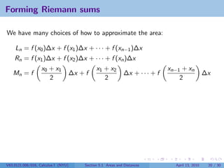
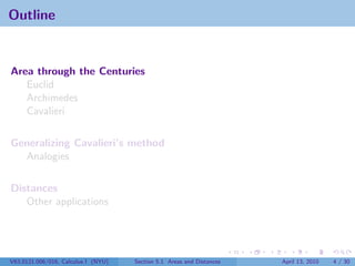
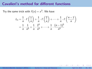
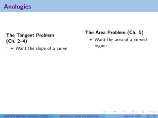
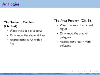
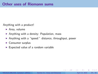
![Forming Riemann sums
We have many choices of how to approximate the area:
Ln = f (x0 )∆x + f (x1 )∆x + · · · + f (xn−1 )∆x
Rn = f (x1 )∆x + f (x2 )∆x + · · · + f (xn )∆x
x0 + x1 x1 + x2 xn−1 + xn
Mn = f ∆x + f ∆x + · · · + f ∆x
2 2 2
In general, choose ci to be a point in the ith interval [xi−1 , xi ]. Form the
Riemann sum
Sn = f (c1 )∆x + f (c2 )∆x + · · · + f (cn )∆x
n
= f (ci )∆x
i=1
V63.0121.006/016, Calculus I (NYU) Section 5.1 Areas and Distances April 13, 2010 20 / 30](https://image.slidesharecdn.com/lesson22-areasanddistancesslides-100413152044-phpapp02/85/Lesson-22-Areas-and-Distances-57-320.jpg)
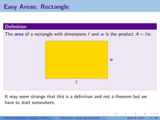
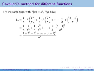
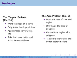
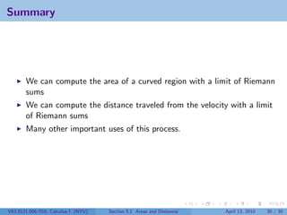
![Theorem of the Day
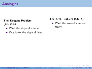
Theorem
If f is a continuous function or
has finitely many jump
discontinuities on [a, b], then
n
lim Sn = lim f (ci )∆x
n→∞ n→∞
i=1
exists and is the same value no
a b
x1
matter what choice of ci we
made.
V63.0121.006/016, Calculus I (NYU) Section 5.1 Areas and Distances April 13, 2010 21 / 30](https://image.slidesharecdn.com/lesson22-areasanddistancesslides-100413152044-phpapp02/85/Lesson-22-Areas-and-Distances-58-320.jpg)
![Theorem of the Day
Theorem
If f is a continuous function or
has finitely many jump
discontinuities on [a, b], then
n
lim Sn = lim f (ci )∆x
n→∞ n→∞
i=1
exists and is the same value no
a x1 b
x2
matter what choice of ci we
made.
V63.0121.006/016, Calculus I (NYU) Section 5.1 Areas and Distances April 13, 2010 21 / 30](https://image.slidesharecdn.com/lesson22-areasanddistancesslides-100413152044-phpapp02/85/Lesson-22-Areas-and-Distances-59-320.jpg)
![Theorem of the Day
Theorem
If f is a continuous function or
has finitely many jump
discontinuities on [a, b], then
n
lim Sn = lim f (ci )∆x
n→∞ n→∞
i=1
exists and is the same value no
a x1 x2 b
x3
matter what choice of ci we
made.
V63.0121.006/016, Calculus I (NYU) Section 5.1 Areas and Distances April 13, 2010 21 / 30](https://image.slidesharecdn.com/lesson22-areasanddistancesslides-100413152044-phpapp02/85/Lesson-22-Areas-and-Distances-60-320.jpg)
![Theorem of the Day
Theorem
If f is a continuous function or
has finitely many jump
discontinuities on [a, b], then
n
lim Sn = lim f (ci )∆x
n→∞ n→∞
i=1
exists and is the same value no
a x1 x2 x3 b
x4
matter what choice of ci we
made.
V63.0121.006/016, Calculus I (NYU) Section 5.1 Areas and Distances April 13, 2010 21 / 30](https://image.slidesharecdn.com/lesson22-areasanddistancesslides-100413152044-phpapp02/85/Lesson-22-Areas-and-Distances-61-320.jpg)
![Theorem of the Day
Theorem
If f is a continuous function or
has finitely many jump
discontinuities on [a, b], then
n
lim Sn = lim f (ci )∆x
n→∞ n→∞
i=1
exists and is the same value no
a x x x x x
matter what choice of ci we 1 2 3 4 b5
made.
V63.0121.006/016, Calculus I (NYU) Section 5.1 Areas and Distances April 13, 2010 21 / 30](https://image.slidesharecdn.com/lesson22-areasanddistancesslides-100413152044-phpapp02/85/Lesson-22-Areas-and-Distances-62-320.jpg)
![Theorem of the Day
Theorem
If f is a continuous function or
has finitely many jump
discontinuities on [a, b], then
n
lim Sn = lim f (ci )∆x
n→∞ n→∞
i=1
exists and is the same value no
a x x x x x x
matter what choice of ci we 1 2 3 4 5 b6
made.
V63.0121.006/016, Calculus I (NYU) Section 5.1 Areas and Distances April 13, 2010 21 / 30](https://image.slidesharecdn.com/lesson22-areasanddistancesslides-100413152044-phpapp02/85/Lesson-22-Areas-and-Distances-63-320.jpg)
![Theorem of the Day
Theorem
If f is a continuous function or
has finitely many jump
discontinuities on [a, b], then
n
lim Sn = lim f (ci )∆x
n→∞ n→∞
i=1
exists and is the same value no
a x x x x x x x
matter what choice of ci we 1 2 3 4 5 6 b7
made.
V63.0121.006/016, Calculus I (NYU) Section 5.1 Areas and Distances April 13, 2010 21 / 30](https://image.slidesharecdn.com/lesson22-areasanddistancesslides-100413152044-phpapp02/85/Lesson-22-Areas-and-Distances-64-320.jpg)
![Theorem of the Day
Theorem
If f is a continuous function or
has finitely many jump
discontinuities on [a, b], then
n
lim Sn = lim f (ci )∆x
n→∞ n→∞
i=1
exists and is the same value no
ax x x x x x x x
matter what choice of ci we 1 2 3 4 5 6 7 b8
made.
V63.0121.006/016, Calculus I (NYU) Section 5.1 Areas and Distances April 13, 2010 21 / 30](https://image.slidesharecdn.com/lesson22-areasanddistancesslides-100413152044-phpapp02/85/Lesson-22-Areas-and-Distances-65-320.jpg)
![Theorem of the Day
Theorem
If f is a continuous function or
has finitely many jump
discontinuities on [a, b], then
n
lim Sn = lim f (ci )∆x
n→∞ n→∞
i=1
exists and is the same value no
ax x x x x x x x x
matter what choice of ci we 1 2 3 4 5 6 7 8b9
made.
V63.0121.006/016, Calculus I (NYU) Section 5.1 Areas and Distances April 13, 2010 21 / 30](https://image.slidesharecdn.com/lesson22-areasanddistancesslides-100413152044-phpapp02/85/Lesson-22-Areas-and-Distances-66-320.jpg)
![Theorem of the Day
Theorem
If f is a continuous function or
has finitely many jump
discontinuities on [a, b], then
n
lim Sn = lim f (ci )∆x
n→∞ n→∞
i=1
exists and is the same value no
a x x x x x x x x x xb
matter what choice of ci we 1 2 3 4 5 6 7 8 9 10
made.
V63.0121.006/016, Calculus I (NYU) Section 5.1 Areas and Distances April 13, 2010 21 / 30](https://image.slidesharecdn.com/lesson22-areasanddistancesslides-100413152044-phpapp02/85/Lesson-22-Areas-and-Distances-67-320.jpg)
![Theorem of the Day
Theorem
If f is a continuous function or
has finitely many jump
discontinuities on [a, b], then
n
lim Sn = lim f (ci )∆x
n→∞ n→∞
i=1
exists and is the same value no
ax x x x x x x x x x xb
matter what choice of ci we 1 2 3 4 5 6 7 8 9 1011
made.
V63.0121.006/016, Calculus I (NYU) Section 5.1 Areas and Distances April 13, 2010 21 / 30](https://image.slidesharecdn.com/lesson22-areasanddistancesslides-100413152044-phpapp02/85/Lesson-22-Areas-and-Distances-68-320.jpg)
![Theorem of the Day
Theorem
If f is a continuous function or
has finitely many jump
discontinuities on [a, b], then
n
lim Sn = lim f (ci )∆x
n→∞ n→∞
i=1
exists and is the same value no
ax x x x x x x x xx x xb
matter what choice of ci we 1 2 3 4 5 6 7 8 9 101112
made.
V63.0121.006/016, Calculus I (NYU) Section 5.1 Areas and Distances April 13, 2010 21 / 30](https://image.slidesharecdn.com/lesson22-areasanddistancesslides-100413152044-phpapp02/85/Lesson-22-Areas-and-Distances-69-320.jpg)
![Theorem of the Day
Theorem
If f is a continuous function or
has finitely many jump
discontinuities on [a, b], then
n
lim Sn = lim f (ci )∆x
n→∞ n→∞
i=1
exists and is the same value no
ax x x x x x x x xx x x xb
matter what choice of ci we 1 2 3 4 5 6 7 8 910 12
11 13
made.
V63.0121.006/016, Calculus I (NYU) Section 5.1 Areas and Distances April 13, 2010 21 / 30](https://image.slidesharecdn.com/lesson22-areasanddistancesslides-100413152044-phpapp02/85/Lesson-22-Areas-and-Distances-70-320.jpg)
![Theorem of the Day
Theorem
If f is a continuous function or
has finitely many jump
discontinuities on [a, b], then
n
lim Sn = lim f (ci )∆x
n→∞ n→∞
i=1
exists and is the same value no
ax x x x x x x x xx x x x xb
matter what choice of ci we 1 2 3 4 5 6 7 8 910 12 14
11 13
made.
V63.0121.006/016, Calculus I (NYU) Section 5.1 Areas and Distances April 13, 2010 21 / 30](https://image.slidesharecdn.com/lesson22-areasanddistancesslides-100413152044-phpapp02/85/Lesson-22-Areas-and-Distances-71-320.jpg)
![Theorem of the Day
Theorem
If f is a continuous function or
has finitely many jump
discontinuities on [a, b], then
n
lim Sn = lim f (ci )∆x
n→∞ n→∞
i=1
exists and is the same value no
ax x x x x x x x xx x x x x xb
matter what choice of ci we 1 2 3 4 5 6 7 8 910 12 14
11 13 15
made.
V63.0121.006/016, Calculus I (NYU) Section 5.1 Areas and Distances April 13, 2010 21 / 30](https://image.slidesharecdn.com/lesson22-areasanddistancesslides-100413152044-phpapp02/85/Lesson-22-Areas-and-Distances-72-320.jpg)
![Theorem of the Day
Theorem
If f is a continuous function or
has finitely many jump
discontinuities on [a, b], then
n
lim Sn = lim f (ci )∆x
n→∞ n→∞
i=1
exists and is the same value no
axxxxxxxxxxxxxxxxb
matter what choice of ci we 1 2 3 4 5 6 7 8 910 12 14 16
11 13 15
made.
V63.0121.006/016, Calculus I (NYU) Section 5.1 Areas and Distances April 13, 2010 21 / 30](https://image.slidesharecdn.com/lesson22-areasanddistancesslides-100413152044-phpapp02/85/Lesson-22-Areas-and-Distances-73-320.jpg)
![Theorem of the Day
Theorem
If f is a continuous function or
has finitely many jump
discontinuities on [a, b], then
n
lim Sn = lim f (ci )∆x
n→∞ n→∞
i=1
exists and is the same value no
a xxxxxxxxxxxxxxxxb
x1 2 3 4 5 6 7 8 910 12 14 16
matter what choice of ci we 11 13 15 17
made.
V63.0121.006/016, Calculus I (NYU) Section 5.1 Areas and Distances April 13, 2010 21 / 30](https://image.slidesharecdn.com/lesson22-areasanddistancesslides-100413152044-phpapp02/85/Lesson-22-Areas-and-Distances-74-320.jpg)
![Theorem of the Day
Theorem
If f is a continuous function or
has finitely many jump
discontinuities on [a, b], then
n
lim Sn = lim f (ci )∆x
n→∞ n→∞
i=1
exists and is the same value no
a xxxxxxxx xxxxxxxxb
x1 2 3 4 5 6 7 8x10 12 14 16 18
matter what choice of ci we 9 11 13 15 17
made.
V63.0121.006/016, Calculus I (NYU) Section 5.1 Areas and Distances April 13, 2010 21 / 30](https://image.slidesharecdn.com/lesson22-areasanddistancesslides-100413152044-phpapp02/85/Lesson-22-Areas-and-Distances-75-320.jpg)
![Theorem of the Day
Theorem
If f is a continuous function or
has finitely many jump
discontinuities on [a, b], then
n
lim Sn = lim f (ci )∆x
n→∞ n→∞
i=1
exists and is the same value no
a xxxxxxxx xxxxxxxxxb
x12345678910 12 14 16 18
x 11 13 15 17 19
matter what choice of ci we
made.
V63.0121.006/016, Calculus I (NYU) Section 5.1 Areas and Distances April 13, 2010 21 / 30](https://image.slidesharecdn.com/lesson22-areasanddistancesslides-100413152044-phpapp02/85/Lesson-22-Areas-and-Distances-76-320.jpg)
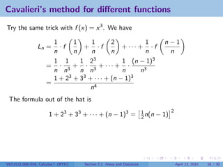
![Theorem of the Day
Theorem
If f is a continuous function or
has finitely many jump
discontinuities on [a, b], then
n
lim Sn = lim f (ci )∆x
n→∞ n→∞
i=1
exists and is the same value no
a xxxxxxxx xxxxxxxxxxb
x123456789101214161820
x 1113151719
matter what choice of ci we
made.
V63.0121.006/016, Calculus I (NYU) Section 5.1 Areas and Distances April 13, 2010 21 / 30](https://image.slidesharecdn.com/lesson22-areasanddistancesslides-100413152044-phpapp02/85/Lesson-22-Areas-and-Distances-77-320.jpg)
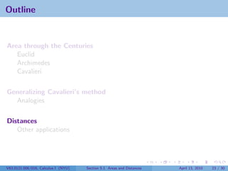

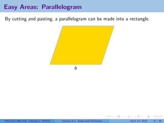
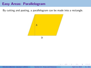
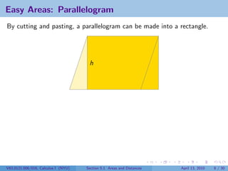
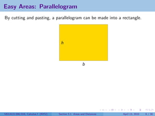
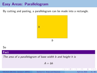
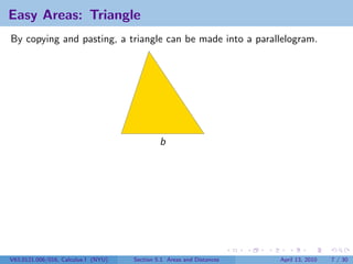
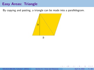
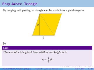
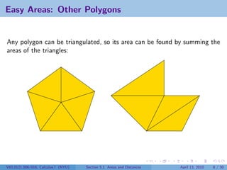
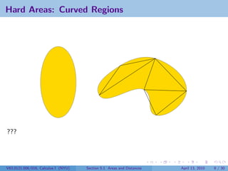
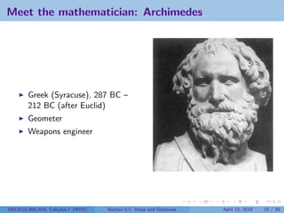
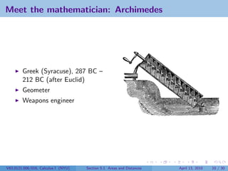
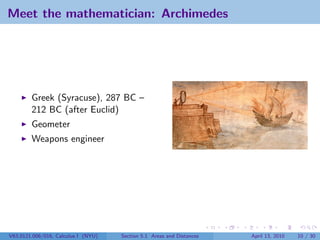
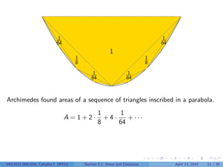
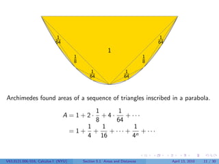
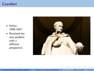
This document outlines the content of a Calculus I course at New York University, focusing on areas and distances as of April 13, 2010. It includes objectives such as computing area using rectangles and determining total distance traveled by a particle. The document also discusses mathematical concepts from historical figures like Euclid, Archimedes, and Cavalieri, and techniques for calculating areas of various shapes.


