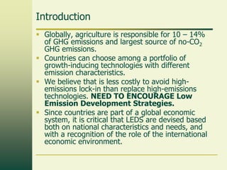
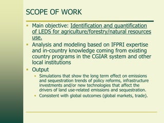
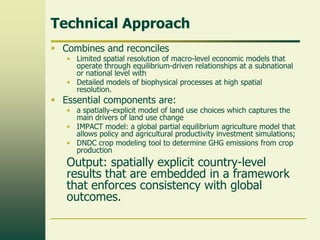
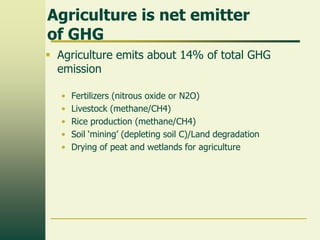
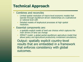
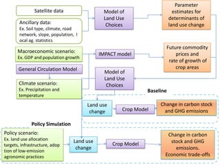
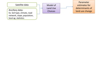
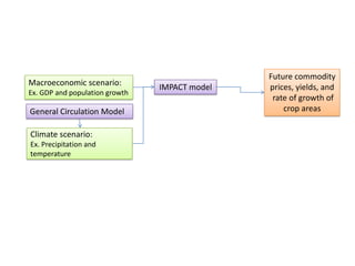
Technical Training for Modeling
Scenarios for
Low Emission Development
Strategies
Alex De Pinto - Senior Research Fellow
Dr. Tim Thomas - Research Fellow
Dr. Man Li - Research Fellow
Dr. Ho-Young Kwon - Research Fellow
Ms. Akiko Haruna - Senior Research Assistant
Ms. Shahnila Islam - Senior Research Assistant
Mr. Daniel Mason – D’Croz - Research Analyst
Ms. Subhashini Mesipam - Administrative Coordinator
INTERNATIONAL FOOD POLICY RESEARCH INSTITUTE
FROM GLOBAL TO LOCAL:
AN INTEGRATED APPROACH TO
LOW EMISSIONS
DEVELOPMENT STRATEGIES
(LEDS)
Alex De Pinto - Senior Research Fellow
Dr. Tim Thomas - Research Fellow
Dr. Man Li - Research Fellow
Dr. Ho-Young Kwon - Research Fellow
Ms. Akiko Haruna - Senior Research Assistant
Ms. Shahnila Islam - Senior Research Assistant
Mr. Daniel Mason – D’Croz - Research Analyst
Ms. Subhashini Mesipam - Administrative
Coordinator
INTERNATIONAL FOOD POLICY RESEARCH INSTITUTE
Introduction
 Globally, agriculture is responsible for 10 – 14%
of GHG emissions and largest source of no-CO2
GHG emissions.
 Countries can choose among a portfolio of
growth-inducing technologies with different
emission characteristics.
 We believe that is less costly to avoid highemissions lock-in than replace high-emissions
technologies. NEED TO ENCOURAGE Low
Emission Development Strategies.
 Since countries are part of a global economic
system, it is critical that LEDS are devised based
both on national characteristics and needs, and
with a recognition of the role of the international
economic environment.
SCOPE OF WORK
 Main objective: Identification and quantification
of LEDS for agriculture/forestry/natural resources
use.
 Analysis and modeling based on IFPRI expertise
and in-country knowledge coming from existing
country programs in the CGIAR system and other
local institutions
 Output
• Simulations that show the long term effect on emissions
and sequestration trends of policy reforms, infrastructure
investments and/or new technologies that affect the
drivers of land use-related emissions and sequestration.
• Consistent with global outcomes (global markets, trade).
Technical Approach
 Combines and reconciles

• Limited spatial resolution of macro-level economic models that
operate through equilibrium-driven relationships at a subnational
or national level with
• Detailed models of biophysical processes at high spatial
resolution.

 Essential components are:

• a spatially-explicit model of land use choices which captures the
main drivers of land use change
• IMPACT model: a global partial equilibrium agriculture model that
allows policy and agricultural productivity investment simulations;
• DNDC crop modeling tool to determine GHG emissions from crop
production

Output: spatially explicit country-level
results that are embedded in a framework
that enforces consistency with global
outcomes.
Climate Change
Mitigation in the
Agricultural Sector

INTERNATIONAL FOOD POLICY RESEARCH INSTITUTE
Agriculture is net emitter
of GHG
 Agriculture emits about 14% of total GHG
emission
•
•
•
•
•

Fertilizers (nitrous oxide or N2O)
Livestock (methane/CH4)
Rice production (methane/CH4)
Soil „mining‟ (depleting soil C)/Land degradation
Drying of peat and wetlands for agriculture
Agriculture and
Mitigation Potential
 Agriculture can also help reducing GHG
emission
MITIGATION:
Climate change mitigation refers to actions that reduce the
potentially harmful effects of global warming by reducing
the atmospheric concentration of GHG.
Different ideas about Agriculture
and Mitigation Potential

A brief review of key
terminology







Adaptation
Additionality
Baseline
Leakage
Monitoring Reporting and Verification
Permanence
A brief Review of key
terminology
 Adaptation: Climate change adaptation
refers to a set of actions, strategies,
processes, and policies that respond to actual
or expected climate changes so that the
consequences for individuals, communities,
and economy are minimized.
 Additionality: A project is said to meet the
additionality criterion if the carbon
sequestration or emission reductions achieved
by the project would not have been
obtained in absence of the project.
Pag
e
11
A brief Review of key
terminology
 Baseline: The baseline scenario describes
GHG emissions in the absence of a project or
a policy.
 Leakage: The adoption of certain
agricultural practices may reduce emissions in
a given area or region; however, these
emission savings could be negated if the type
of agricultural production a project is trying to
prevent shifts to other regions.

Pag
e
12
A brief Review of key
terminology

 Permanence: This concept is related to the length of
time the carbon sequestration or reduction of
emissions last. The objective is to assure that the
mitigation service is provided for the entire length of a
project. Permanence raises significant issues related
to opportunity costs.
 Measurement Reporting and Verification (MRV):
• Measurement: “The process of data collection over time,
providing basic datasets, including associated accuracy and
precision, for the range of relevant variables. Possible data
sources are field measurements, field observations, detection
through remote sensing and interviews.”
• Reporting: “The process of formal reporting of assessment results
according to predetermined formats and according to established
standards”
• Verification: “The process of formal verification of reports, for
example, the established approach to verify national
communications and national inventory reports to the UNFCCC.”

Pag
e
13
Global mitigation potential in
agriculture

Total technical mitigation potentials (all practices, all GHGs: MtCO2-eq/yr) for each region by 2030.
Note: based on the B2 scenario though the pattern is similar for all SRES scenarios.
Source: Smith et al. (2007)
We can do much better now

Pag
e
15
Agriculture can play a role in
mitigating climate change
 Modifying and introducing agricultural practices
and crop patterns so that:
• Sequester CO2 from atmosphere and store it soils (or trees –
agroforestry)
• Reduce GHG emissions

 It is obvious that most if not all modifications to
agricultural practices will have effects, positive
and negative, on output and will have
effects, positive and negative, of the economics of
these activities (i.e. profit)
Challenges and Opportunities
 Potential Opportunities (????)
• Provide farmers with an additional source of income –
carbon markets
• Help small poor farmers dealing with the effects of
climate change (co-benefit)
• Food security and resilience (co-benefit)

 Challenges
• Uncertainty in the amounts of GHG that can be
reduced, but also pemanence, MRV, lekeage
• Uncertainty in the economic effects that mitigation
policies might have
Co-benefits of mitigation
 Mitigation practices overlap considerably with
sustainable use of resources. Could be
interpreted as an increase of overall efficiency of
the production system.
 Positive correlation between soil C and crop
yield. Some agricultural practices improve soil
fertility and induce C sequestration
 More efficient water use (reduces CO2 from
fuel/electricity) and methane from rice paddy
 Agricultural R&D, advisory services, and
information systems
Consideration about mitigation and
adaptation
 Many people make a clear distinction
between mitigation and adaptation.
 In many instances mitigation
practices are good adaptation
practices.
 Mitigation as a path towards
adaptation.
Constraints to climate change
mitigation using agriculture
 Growing literature on the difficulties for agriculture
to contribute to mitigation:

•
•
•
•
•
•
•

Defining the baseline
Biophysical Modeling
Evidence of additionality
Profitability
High transaction costs SocioeconomicAnalysis
Property rights
Leakage
Wider Scale Modeling
Permanence
Constraints to climate change
mitigation using agriculture

Biophysical Modeling
• Defining the baseline
• Evidence of additionality
Emissions – CO2 eq

Constraints to climate change mitigation
using agriculture: Biophysical
BASELINE

Emissions with business as usual

Mitigation potential
Additionality

Emissions with mitigation option

Time

Pag
e
22
Defining the Baseline
 Forestry - one has to be able to “reliably”
project the future of a forest in absence of a
project.
 Agriculture - most important cropping
systems, production practices, need to be
identified:
• Easy for an American farmer who grows soybeansmaize year after year
• Easy for a Vietnamese farmer who only grows rice year
after year
• Difficult for a smallholder who utilizes complex cropping
systems that change in time: an example from some
African countries where cropping systems like maizecocoyam-cassava-plantain-fallow are the norm
Defining the Baseline
Geophysical
characteristics
Most
common/important
crops

Climate
scenarios

A
Crop
model

Climate
scenarios

B

Geophysical
characteristics

Mitigation Ag.
practices/input
package

A-B
Mitigation
potential

Current Ag.
practices

Most
common/important
crops

Carbon
baseline

Crop
model

Carbon profile
input package #1
Carbon profile
input package #2

.
.
Carbon profile
input package #n
Emissions and Carbon Stock (CO2 eq.)

Carbon stock and
GHG emissions computed
from simulations for
baseline

Growth in carbon stock and
GHG emissions extrapolated
from 2009 and 2030 values

Increase in Carbon stock
2009 – 2030
Carbon stock baseline
Emissions baseline

Increase in emissions
2009 – 2030 area ABC

C

A
B

2009

2030

Time
Assessing climate change mitigation
potential in agriculture
Key Modeling Issues
 How good are crop models?


Knowledge / quantification of how different agronomic
practices and different crops affect GHG emissions
(DSSAT/Century, DNDC, CropSys, EPIC, APSIM).

 How good is our ability to generate plausible scenarios of
future land-use choices, crop choices, agronomic practices
(surveys, models of land-use change).
 Major obstacle: creating a baseline. Predicting
smallholders behavior is challenging.
Constraints to climate change
mitigation using agriculture

Socioeconomic
Analysis
• Profitability – Will farmers be better off?
• Society-wide benefits – Will society be
better off?
Some Economic Results - Vietnam
1450

CH4 & N2O Emissions
(CO2eq/ha)

1400
1350
1300
1250
1200
1150
1100
1050
Conventional

New variety

Biochar

Composting

AWD irrigation

New variety

Biochar

Composting

AWD irrigation

200
150

50
0
Conventional
-50

-100
-150
-200
-250

High labor cost
to produce and
spread

Net profit (US$/ha)
compared to
Conventional

100
Some Economic Results - Ghana
Manure/Nitrogen

Carbon Accumulation,

Total Payment/Implicit

Yield Gains

applications

end of 20 yr period

Cost of Carbon

Maize/Cassava

Risk-neutral agent

Dry Weight

(USD/ha)

(Kg/ha)

(Kg/ha)

(Ton CO2 eq/ha)

250/0

0.31

207/670

40/162

500/0

0.45

456/278

58/290

750/0

0.81

732/247

74/406

1,000/0

1.16

1,000/235

88/509

250/60

2.16

73/34

215/950

500/60

3.40

220/65

215/1,14

750/60

4.63

462/100

214/1,071

1,000/60

5.85

719/123

215/1,134
Some Economic Results - Morocco

Method

Traditional
Soft
Wheat

NPV
1,000 US $
(r = 8%)
5.9

Necessary
Investment
(1,000 US$)

Yearly
Reduction in
Average
CO2
Carbon
Emissions
Accumulation

6.8

Zero Tillage

13. 9

7.2

Traditional
irrigation

8.1

1.8 Tons
CO2eq/year

0.9 Tons
CO2eq/year

3.2
-

Drip irrigation

55.8
5.0

3.2

Drip irrigation

51.8

0.4 Tons
CO2eq/year

16.8

Traditional
irrigation

0.3 Tons
CO2eq/year

-

Potato

Onion
16.8
Expanding the Analysis Using the Time
Dimension - Ghana

Financial support
can be removed
and alternatives
more profitable
that baseline
Expanding the Analysis Using the Time
Dimension - Mozambique
Minimum incentive (USD, per ha), present value at the each payment period
Column1

1st cycle

2nd cycle

3rd cycle

4th cycle

No-till

101

192

322

to add 500 kg ha-1 farm yard manure to each crop (38.5 kg N ha-1)

309

0

0

to add 60 kg N ha-1 chemical fertilizer nitrate

0

0

0

0

500 kg manure +60kg nitrate + no-till

0

0

0

0

332

0

0

0)

1000 kg manure +60kg nitrate + no-till;

566
Overall Lessons Learned:

Pilot Study and Cost Benefit Analysis of Alternate
Mitigation Practices

 Productivity growth, increased sustainable
production, reduction in GHG emissions, are
not mutually exclusive choices.
 Lack of credit, investments costs, and risk
aversion create a substantial barriers to the
adoption of mitigation practices.
 Compensation for mitigation services
facilitates the adoption of agronomic practices
that allow sustainable intensification.
Role of Uncertainty and Risk
 There is plenty of evidence that farmers are not
likely to be neutral to risk and actually tend to be
risk averse (Antle 1987; Chavas and Holt 1990;
Bar-Shira, Just, and Zilberman 1997; Hennessy
1998; Just and Pope 2002; Serra et al. 2006;
Yesuf and Bluffstone 2007)
 and that risk considerations affect input usage
and technology adoption (Just and Zilberman
1983; Feder, Just, and Zilberman 1985; Kebede
1992).
 Risk considerations should not be ignored in the
analysis of adoption of carbon sequestration
practices.
Implementation Challenges
 Implementation challenges
• costs involved in organizing farmers (aggregation
process)
• costs of empowering farmers with the necessary
knowledge
• costs of Monitoring, Reporting and Verification (MRV)

 Need for strong institutional support.
Institutions should include the potential of
various supply chains, producers of high value
export crops, non-governmental organizations
(NGOs), and farmer organizations as aggregators
and disseminators of management system
changes and measurement technologies
Your Opinion on Agriculture
and Mitigation Potential

Your Opinion on Agriculture
and Mitigation Potential

IFPRI’s Approach
Modeling Setting and Data

Pag
e
38
Technical Approach
 Combines and reconciles
• Limited spatial resolution of macro-level economic models that
operate through equilibrium-driven relationships at a subnational
or national level with
• Detailed models of biophysical processes at high spatial
resolution.

 Essential components are:
• a spatially-explicit model of land use choices which captures the
main drivers of land use change
• IMPACT model: a global partial equilibrium agriculture model that
allows policy and agricultural productivity investment simulations;

Output: spatially explicit country-level
results that are embedded in a framework
that enforces consistency with global
outcomes.
Satellite data

Parameter
estimates for
determinants of
land use change

Model of
Land Use
Choices

Ancillary data:
Ex. Soil type, climate, road
network, slope, population, l
ocal ag. statistics

Macroeconomic scenario:

Future commodity
prices and
rate of growth of
crop areas

IMPACT model

Ex. GDP and population growth

General Circulation Model

Model of
Land Use
Choices

Climate scenario:
Ex. Precipitation and
temperature

Baseline
Land use
change

Crop Model

Change in carbon stock
and GHG emissions

Policy Simulation

Policy scenario:
Ex. land use allocation
targets, infrastructure, adop
tion of low-emission
agronomic practices

Land use
change

Crop Model

Change in carbon
stock and GHG
emissions.
Economic trade-offs
Satellite data
Ancillary data:
Ex. Soil type, climate, road
network, slope, population,
local ag. statistics

Model of
Land Use
Choices

Parameter
estimates for
determinants of
land use change
Macroeconomic scenario:
Ex. GDP and population growth

General Circulation Model
Climate scenario:
Ex. Precipitation and
temperature

IMPACT model

Future commodity
prices, yields, and
rate of growth of
crop areas
Satellite data
Ancillary data:
Ex. Soil type, climate, road
network, slope, population,
local ag. statistics

Macroeconomic scenario:
Ex. GDP and population growth

General Circulation Model
Climate scenario:
Ex. Precipitation and
temperature

Parameter
estimates for
determinants of
land use change

Model of
Land Use
Choices

Future commodity
prices and
rate of growth of
crop areas

IMPACT model
Model of
Land Use
Choices

Baseline
Land use
change

Crop Model

Change in carbon stock
and GHG emissions
Satellite data

Parameter
estimates for
determinants of
land use change

Model of
Land Use
Choices

Ancillary data:
Ex. Soil type, climate, road
network, slope, population,
local ag. statistics

Macroeconomic scenario:

Future commodity
prices and
rate of growth of
crop areas

IMPACT model

Ex. GDP and population growth

General Circulation Model

Model of
Land Use
Choices

Climate scenario:
Ex. Precipitation and
temperature

Baseline
Land use
change

Crop Model

Change in carbon stock
and GHG emissions

Policy Simulation

Policy scenario:
Ex. land use allocation
targets, infrastructure,
adoption of low-emission
agronomic practices

Land use
change

Crop Model

Change in carbon
stock and GHG
emissions.
Economic trade-offs
Baseline: Land cover – MODIS 2009
Climate change 2009 – 2030

Change in annual precipitation, 2009 to 2030
(CSIRO Climate Model)

Change in annual mean temperature, 2009 to
2030 (CSIRO Climate Model)
Assumptions in baseline scenario
Time period 2009 - 2030
 GDP – IMPACT medium variant
 Population – UN pop medium variant
 Exogenous productivity and area growth –
IMPACT standard
 Climate – CSIRO GCM, A1B scenario
Typical Modeling
Output

Pag
e
48
Baseline Scenario Price Changes
2009-2030
Price (USD/ton)

Yield (ton/ha)

a

b

Area
growth
(%) c

2009

Bean
Cassava
Cotton
Groundnuts
Maize
Irrigated Rice
Rainfed Rice
Soybean
Sugar cane
Sweet potato
Coffee

2030

Growth (% )

2009

2030

Growth (%)

523

577

10.16%

0.95

1.01

6.69%

8.67%

54

73

35.54%

16.80

20.40

21.40%

1.40%

898

1132

26.02%

1.33

1.57

17.78%

0.00%

512

577

12.73%

2.09

2.41

15.25%

-0.63%

53

74

39.01%

4.10

5.74

39.93%

1.73%

133

167

25.89%

5.19

5.90

13.69%

-1.71%

133

167

25.89%

2.87

3.27

13.69%

-1.71%

154

198

28.60%

1.46

1.41

-3.13%

-2.18%

13

17

27.32%

58.77

66.34

12.88%

43.68%

433

531

22.72%

8.26

12.25

48.33%

-3.33%

806

897

11.39%

2.08

2.22

6.69%

8.67%

Source: IMPACT.
Land Use Change 2009 - 2030
Baseline scenario
Land Use Category

2009 land area
(Million Hectares)

2030 land area
(Million Hectares)

Change in Area
2009 - 2030
(Million ha)

Cropland

5.05

5.14

0.10

Mosaic

6.52

6.72

0.20

Woody Savannas

6.22

5.29

-0.93

Forest

12.65

12.96

0.31

Shrub/Grassland

0.47

0.51

0.04

Other Land Uses

1.93

2.22

0.29

Total

32.84

32.84

0.00
Land Use 2030 – Baseline scenario
2009 area

2030 area

Change in Area

(ha)

Crops

(ha)

2009 – 2030
(ha)

Beans

187,200

203,437

16,237

Cassava

507,800

514,894

7,094

Cotton

9,600

9,600

0

Groundnuts

245,000

243,468

-1,532

Maize

1,089,200

1,108,073

18,873

Irrigated Rice

6,892,600

6,774,615

-117,985

Rainfed Rice

546,000

536,654

-9,346

Soybeans

131,900

129,018

-2,882

Sugarcane

265,600

381,612

116,012

Sweet Potato

146,400

141,524

-4,876

Coffee

538,400

585,100

46,700

Total

10,559,700

10,627,996

68,296
Pag
e
51
Land Use 2030 – Baseline Scenario

Land use conversion: Change in forested land.
Year 2009 – 2030

Land use conversion: Change in agricultural land.
Year 2009 – 2030
GHG Emissions and Carbon Stock
Below
ground
carbon
stock b

YES

Land Use
Category

Above
ground
carbon
stock a

YES

YES

YES

YES

YES

YES

YES

YES

YES

YES

YES

YES

YES

YES

YES

YES

YES

YES

YES

YES

YES

YES

YES

SOC

c

CO2 d

N2O

d

CH4 d

Cropland
Mosaic
Woody
Savannas
Forest
Shrub/Grassl
and
Other Land
Uses
Page 54

ANALYSIS OF THE RESULTS

INTERNATIONAL FOOD POLICY RESEARCH INSTITUTE
Carbon Stock – Changes 2009 - 2030
Land Use
Category

Soil
Organic
Carbon
2009
(Tg C)

Above
Ground
Biomass
2009
(Tg C)

Below
Ground
Biomass
2009
(Tg C)

Soil
Organic
Carbon
2030
(Tg C)

Above
Ground
Biomass
2030
(Tg C)

Below
Ground
Biomass
2030
(Tg C)

Net
Change in
Carbon
Stock
2009 2030
(Tg C)

Cropland

286.3

-

-

287.0

-

-

0.7

Mosaic
Woody
Savannas
Forest

294.0
246.2

135.6
29.1

33.5
15.0

298.9
208.8

148.0
25.7

36.4
13.9

20.2
-41.8

520.9

989.3

232.9

532.8

1,015.8

239.2

44.7

Shrub/Grassl
and

22.7

4.2

1.7

24.5

4.6

1.8

2.2

Other Land
Uses
Total

139.1

-

-

161.0

-

-

21.9

1,509.2

1,158.2

283.0

1,512.9

1,194.1

291.4

47.9
GHG Emissions – Changes 2009 - 2030
Per ha GHG
emission

2009 total GHG
emission

2030 total GHG
emission

(ton/ha)

(Tg CO2eq year-1)

(Tg CO2eq
year-1)

Beans

14.81

2.77

3.01

0.24

Cassava

14.87

7.55

7.64

0.09

Cotton

0.47

0.00

0.00

0

Groundnuts

10.62

2.60

2.58

-0.02

Maize

7.21

7.86

7.98

0.12

Irrigated Rice

21.21

146.17

143.82

-2.34

Rainfed Rice

21.37

11.67

11.47

-0.20

Soybeans

14.81

1.95

1.91

-0.04

Sugarcane

35.58

9.45

13.56

4.11

Sweet Potato

0.33

0.05

0.05

-0.002

Coffee

0.56

0.30

0.33

0.02

190.37

192.35

1.98

Crops

Total

Changes in
total GHG
emission
2009 - 2030
(Tg CO2eq)
Baseline Results
 Carbon stock increases at an annual rate of
0.08% while GHG emission increase at a rate
of 0.04% annually.
 Increase in GHG emissions deriving from
changes in crop production are
counterbalanced by an increase in carbon
stock, mainly due to increase in forested
areas.

Pag
e
57
Baseline Results
 Carbon stock increases at an annual rate of
0.08% while GHG emission increase at a rate
of 0.04% annually.
 Increase in GHG emissions deriving from
changes in crop production are
counterbalanced by an increase in carbon
stock, mainly due to increase in forested
areas.

Pag
e
58
Baseline Results - Economy
Crops

Change in Area
2009 – 2030
(ha)

2009 total
revenue

2030 total
revenue

(Million USD)

(Million USD)

Changes in
total revenue
(Million USD)

Beans

16,237

93.2

119.0

25.8

Cassava

7,094

460.9

769.1

308.2

Cotton

0

11.5

17.0

5.6

Groundnuts

-1,532

262.2

338.6

76.4

Maize

18,873

240.1

475.1

235.0

Irrigated Rice

-117,985

4,768.7

6,708.7

1,940.0

Rainfed Rice

-9,346

209.0

294.0

85.0

Soybeans

-2,882

29.7

36.2

6.5

Sugarcane

116,012

211.0

435.8

224.8

Sweet Potato

-4,876

523.7

921.5

397.8

Coffee

46,700

902.7

1,165.8

263.1

Total

68,296

7,712.7

11,280.8

3,568.2

Pag
e
59
Alternative Policies
 Objective: increase forested area
• Forest area would have to increase by an additional 1.6
million hectares compared to the baseline - forest area
increases by 310,000 hectares in the baseline projection
– with a net change in carbon stock equivalent to 510
million tons of CO2eq (the increase in forest carbon
stock of 800 million tons of CO2eq is counterbalanced a
by loss in stock from other land uses). The increase in
forested area causes a reduction in cropland area of
about 500,000 hectares with a resulting reduction in
annual GHG emissions from crop production estimated
to be 10.2 million tons of CO2eq and a reduction in
revenue from crop production of 670 million USD
Alternative Policies
 Rice area at 3.5 million hectares – Carbon stock from
all land uses increase by a total of 247 million tons of
CO2eq (an additional 71 million tons of CO2eq compared to
the baseline). Emissions from crop production decrease by
4.4 million tons of CO2eq a year by 2030 (baseline results
project a yearly increase of 1.7 million tons of CO2eq). The
reduction in rice area causes an estimated loss in revenue
equivalent to 154 million USD per year compared to the
baseline .
 Alternative wet and dry management for irrigated
rice – estimated reduction in GHG equivalent to 113 million
tons of CO2eq and a loss in revenue of 271 million USD.
Alternative Policies
 Use of compost manure - estimated reduction in GHG
equivalent to 22 million tons of CO2eq and a loss in
revenue of 530 million USD.
 Ammonium sulfate - estimated reduction in GHG
equivalent to 9 million tons of CO2eq and a gain in revenue
of 130 million USD.

Conclusion
This approach allows us to:
 Determine land use choices trends, pressure for
change in land uses and tension forest/
agriculture
 Simulate policy scenarios, their viability and the
role of market forces
 Simulate the long term effect on emissions and
sequestration trends of the identified policy
reforms in relation to global price changes and
trade policies

Pag
e
63
Conclusion
Next steps and important data needs:
 Include pasture and livestock in the analysis.
 Better inventory of existing carbon stock in
forests
 Include other crops: tea, cocoa, rubber
 Better prices at local markets
 Determine the policy and policy reforms
that Vietnam would like to explore and
simulate

Pag
e
64
Page 65

THANK YOU

INTERNATIONAL FOOD POLICY RESEARCH INSTITUTE
Regulatory Markets
 UN-REDD and REDD+

• Reducing Emissions from Deforestation and Degradation
(REDD)
• REDD+ includes the role of conservation, sustainable
management of forests and enhancement of forest carbon
stocks.
• http://www.un-redd.org/

 Clean Development Mechanism (CDM)
• Exemples of Project accepted:

Biogas recovery and electricity generation from Palm Oil Mill Effluent
 Advanced swine manure treatment
 Methane capture and combustion from poultry manure treatment


• All GHG are considered, demanding and difficult to achieve
• http://cdm.unfccc.int/index.html
Voluntary Markets
 Gold Standard (non-profit organization)
• Examples:



Solar Cookers
Biodigesters

• In essence as demanding as CDM
• http://www.cdmgoldstandard.org/

 Voluntary Carbon Standards (VCS)

• Afforestation, Reforestation and Revegetation (ARR)
• Agricultural Land Management (ALM)
• Improved Forest Management (IFM)
• No approved methodology for agricultural land
management (ALM) yet
• http://www.v-c-s.org/
• Supposed to be more accessible than CDM, GS
Pag
e
67
Voluntary Markets
 Climate Action Reserve (CAR)
• No protocols yet (last time I checked)
• http://www.climateactionreserve.org/

Pag
e
68
Other Sources of Financing
• Nationally Appropriate Mitigation
Actions (NAMAs)
• Locally Appropriate Mitigation Actions
(LAMAs)

Pag
e
69
Concluding Remarks
 Farmers appear to have the potential to make a
meaningful contribution to climate change mitigation.
 Adoption of mitigation practices limited by lack of
credit, required investments and risk reducing
financial mechanisms.
 At the farm level, the distinction between adaptation
and mitigation goals becomes blurry.
 There already are in place organizations that could
facilitate the access to carbon markets. However, their
involvement could be costly given their limited
knowledge of the specifics involved in climate change
mitigation in agriculture.
 Functioning carbon market have the potential to help
poor smallholder farmers.

Low Emissions Development Strategies (LEDS) Training Sept 9, 2013

  • 1.
    Technical Training forModeling Scenarios for Low Emission Development Strategies Alex De Pinto - Senior Research Fellow Dr. Tim Thomas - Research Fellow Dr. Man Li - Research Fellow Dr. Ho-Young Kwon - Research Fellow Ms. Akiko Haruna - Senior Research Assistant Ms. Shahnila Islam - Senior Research Assistant Mr. Daniel Mason – D’Croz - Research Analyst Ms. Subhashini Mesipam - Administrative Coordinator INTERNATIONAL FOOD POLICY RESEARCH INSTITUTE
  • 2.
    FROM GLOBAL TOLOCAL: AN INTEGRATED APPROACH TO LOW EMISSIONS DEVELOPMENT STRATEGIES (LEDS) Alex De Pinto - Senior Research Fellow Dr. Tim Thomas - Research Fellow Dr. Man Li - Research Fellow Dr. Ho-Young Kwon - Research Fellow Ms. Akiko Haruna - Senior Research Assistant Ms. Shahnila Islam - Senior Research Assistant Mr. Daniel Mason – D’Croz - Research Analyst Ms. Subhashini Mesipam - Administrative Coordinator INTERNATIONAL FOOD POLICY RESEARCH INSTITUTE
  • 3.
    Introduction  Globally, agricultureis responsible for 10 – 14% of GHG emissions and largest source of no-CO2 GHG emissions.  Countries can choose among a portfolio of growth-inducing technologies with different emission characteristics.  We believe that is less costly to avoid highemissions lock-in than replace high-emissions technologies. NEED TO ENCOURAGE Low Emission Development Strategies.  Since countries are part of a global economic system, it is critical that LEDS are devised based both on national characteristics and needs, and with a recognition of the role of the international economic environment.
  • 4.
    SCOPE OF WORK Main objective: Identification and quantification of LEDS for agriculture/forestry/natural resources use.  Analysis and modeling based on IFPRI expertise and in-country knowledge coming from existing country programs in the CGIAR system and other local institutions  Output • Simulations that show the long term effect on emissions and sequestration trends of policy reforms, infrastructure investments and/or new technologies that affect the drivers of land use-related emissions and sequestration. • Consistent with global outcomes (global markets, trade).
  • 5.
    Technical Approach  Combinesand reconciles • Limited spatial resolution of macro-level economic models that operate through equilibrium-driven relationships at a subnational or national level with • Detailed models of biophysical processes at high spatial resolution.  Essential components are: • a spatially-explicit model of land use choices which captures the main drivers of land use change • IMPACT model: a global partial equilibrium agriculture model that allows policy and agricultural productivity investment simulations; • DNDC crop modeling tool to determine GHG emissions from crop production Output: spatially explicit country-level results that are embedded in a framework that enforces consistency with global outcomes.
  • 6.
    Climate Change Mitigation inthe Agricultural Sector INTERNATIONAL FOOD POLICY RESEARCH INSTITUTE
  • 7.
    Agriculture is netemitter of GHG  Agriculture emits about 14% of total GHG emission • • • • • Fertilizers (nitrous oxide or N2O) Livestock (methane/CH4) Rice production (methane/CH4) Soil „mining‟ (depleting soil C)/Land degradation Drying of peat and wetlands for agriculture
  • 8.
    Agriculture and Mitigation Potential Agriculture can also help reducing GHG emission MITIGATION: Climate change mitigation refers to actions that reduce the potentially harmful effects of global warming by reducing the atmospheric concentration of GHG.
  • 9.
    Different ideas aboutAgriculture and Mitigation Potential 
  • 10.
    A brief reviewof key terminology       Adaptation Additionality Baseline Leakage Monitoring Reporting and Verification Permanence
  • 11.
    A brief Reviewof key terminology  Adaptation: Climate change adaptation refers to a set of actions, strategies, processes, and policies that respond to actual or expected climate changes so that the consequences for individuals, communities, and economy are minimized.  Additionality: A project is said to meet the additionality criterion if the carbon sequestration or emission reductions achieved by the project would not have been obtained in absence of the project. Pag e 11
  • 12.
    A brief Reviewof key terminology  Baseline: The baseline scenario describes GHG emissions in the absence of a project or a policy.  Leakage: The adoption of certain agricultural practices may reduce emissions in a given area or region; however, these emission savings could be negated if the type of agricultural production a project is trying to prevent shifts to other regions. Pag e 12
  • 13.
    A brief Reviewof key terminology  Permanence: This concept is related to the length of time the carbon sequestration or reduction of emissions last. The objective is to assure that the mitigation service is provided for the entire length of a project. Permanence raises significant issues related to opportunity costs.  Measurement Reporting and Verification (MRV): • Measurement: “The process of data collection over time, providing basic datasets, including associated accuracy and precision, for the range of relevant variables. Possible data sources are field measurements, field observations, detection through remote sensing and interviews.” • Reporting: “The process of formal reporting of assessment results according to predetermined formats and according to established standards” • Verification: “The process of formal verification of reports, for example, the established approach to verify national communications and national inventory reports to the UNFCCC.” Pag e 13
  • 14.
    Global mitigation potentialin agriculture Total technical mitigation potentials (all practices, all GHGs: MtCO2-eq/yr) for each region by 2030. Note: based on the B2 scenario though the pattern is similar for all SRES scenarios. Source: Smith et al. (2007)
  • 15.
    We can domuch better now Pag e 15
  • 16.
    Agriculture can playa role in mitigating climate change  Modifying and introducing agricultural practices and crop patterns so that: • Sequester CO2 from atmosphere and store it soils (or trees – agroforestry) • Reduce GHG emissions  It is obvious that most if not all modifications to agricultural practices will have effects, positive and negative, on output and will have effects, positive and negative, of the economics of these activities (i.e. profit)
  • 17.
    Challenges and Opportunities Potential Opportunities (????) • Provide farmers with an additional source of income – carbon markets • Help small poor farmers dealing with the effects of climate change (co-benefit) • Food security and resilience (co-benefit)  Challenges • Uncertainty in the amounts of GHG that can be reduced, but also pemanence, MRV, lekeage • Uncertainty in the economic effects that mitigation policies might have
  • 18.
    Co-benefits of mitigation Mitigation practices overlap considerably with sustainable use of resources. Could be interpreted as an increase of overall efficiency of the production system.  Positive correlation between soil C and crop yield. Some agricultural practices improve soil fertility and induce C sequestration  More efficient water use (reduces CO2 from fuel/electricity) and methane from rice paddy  Agricultural R&D, advisory services, and information systems
  • 19.
    Consideration about mitigationand adaptation  Many people make a clear distinction between mitigation and adaptation.  In many instances mitigation practices are good adaptation practices.  Mitigation as a path towards adaptation.
  • 20.
    Constraints to climatechange mitigation using agriculture  Growing literature on the difficulties for agriculture to contribute to mitigation: • • • • • • • Defining the baseline Biophysical Modeling Evidence of additionality Profitability High transaction costs SocioeconomicAnalysis Property rights Leakage Wider Scale Modeling Permanence
  • 21.
    Constraints to climatechange mitigation using agriculture Biophysical Modeling • Defining the baseline • Evidence of additionality
  • 22.
    Emissions – CO2eq Constraints to climate change mitigation using agriculture: Biophysical BASELINE Emissions with business as usual Mitigation potential Additionality Emissions with mitigation option Time Pag e 22
  • 23.
    Defining the Baseline Forestry - one has to be able to “reliably” project the future of a forest in absence of a project.  Agriculture - most important cropping systems, production practices, need to be identified: • Easy for an American farmer who grows soybeansmaize year after year • Easy for a Vietnamese farmer who only grows rice year after year • Difficult for a smallholder who utilizes complex cropping systems that change in time: an example from some African countries where cropping systems like maizecocoyam-cassava-plantain-fallow are the norm
  • 24.
    Defining the Baseline Geophysical characteristics Most common/important crops Climate scenarios A Crop model Climate scenarios B Geophysical characteristics MitigationAg. practices/input package A-B Mitigation potential Current Ag. practices Most common/important crops Carbon baseline Crop model Carbon profile input package #1 Carbon profile input package #2 . . Carbon profile input package #n
  • 25.
    Emissions and CarbonStock (CO2 eq.) Carbon stock and GHG emissions computed from simulations for baseline Growth in carbon stock and GHG emissions extrapolated from 2009 and 2030 values Increase in Carbon stock 2009 – 2030 Carbon stock baseline Emissions baseline Increase in emissions 2009 – 2030 area ABC C A B 2009 2030 Time
  • 26.
    Assessing climate changemitigation potential in agriculture Key Modeling Issues  How good are crop models?  Knowledge / quantification of how different agronomic practices and different crops affect GHG emissions (DSSAT/Century, DNDC, CropSys, EPIC, APSIM).  How good is our ability to generate plausible scenarios of future land-use choices, crop choices, agronomic practices (surveys, models of land-use change).  Major obstacle: creating a baseline. Predicting smallholders behavior is challenging.
  • 27.
    Constraints to climatechange mitigation using agriculture Socioeconomic Analysis • Profitability – Will farmers be better off? • Society-wide benefits – Will society be better off?
  • 28.
    Some Economic Results- Vietnam 1450 CH4 & N2O Emissions (CO2eq/ha) 1400 1350 1300 1250 1200 1150 1100 1050 Conventional New variety Biochar Composting AWD irrigation New variety Biochar Composting AWD irrigation 200 150 50 0 Conventional -50 -100 -150 -200 -250 High labor cost to produce and spread Net profit (US$/ha) compared to Conventional 100
  • 29.
    Some Economic Results- Ghana Manure/Nitrogen Carbon Accumulation, Total Payment/Implicit Yield Gains applications end of 20 yr period Cost of Carbon Maize/Cassava Risk-neutral agent Dry Weight (USD/ha) (Kg/ha) (Kg/ha) (Ton CO2 eq/ha) 250/0 0.31 207/670 40/162 500/0 0.45 456/278 58/290 750/0 0.81 732/247 74/406 1,000/0 1.16 1,000/235 88/509 250/60 2.16 73/34 215/950 500/60 3.40 220/65 215/1,14 750/60 4.63 462/100 214/1,071 1,000/60 5.85 719/123 215/1,134
  • 30.
    Some Economic Results- Morocco Method Traditional Soft Wheat NPV 1,000 US $ (r = 8%) 5.9 Necessary Investment (1,000 US$) Yearly Reduction in Average CO2 Carbon Emissions Accumulation 6.8 Zero Tillage 13. 9 7.2 Traditional irrigation 8.1 1.8 Tons CO2eq/year 0.9 Tons CO2eq/year 3.2 - Drip irrigation 55.8 5.0 3.2 Drip irrigation 51.8 0.4 Tons CO2eq/year 16.8 Traditional irrigation 0.3 Tons CO2eq/year - Potato Onion 16.8
  • 31.
    Expanding the AnalysisUsing the Time Dimension - Ghana Financial support can be removed and alternatives more profitable that baseline
  • 32.
    Expanding the AnalysisUsing the Time Dimension - Mozambique Minimum incentive (USD, per ha), present value at the each payment period Column1 1st cycle 2nd cycle 3rd cycle 4th cycle No-till 101 192 322 to add 500 kg ha-1 farm yard manure to each crop (38.5 kg N ha-1) 309 0 0 to add 60 kg N ha-1 chemical fertilizer nitrate 0 0 0 0 500 kg manure +60kg nitrate + no-till 0 0 0 0 332 0 0 0) 1000 kg manure +60kg nitrate + no-till; 566
  • 33.
    Overall Lessons Learned: PilotStudy and Cost Benefit Analysis of Alternate Mitigation Practices  Productivity growth, increased sustainable production, reduction in GHG emissions, are not mutually exclusive choices.  Lack of credit, investments costs, and risk aversion create a substantial barriers to the adoption of mitigation practices.  Compensation for mitigation services facilitates the adoption of agronomic practices that allow sustainable intensification.
  • 34.
    Role of Uncertaintyand Risk  There is plenty of evidence that farmers are not likely to be neutral to risk and actually tend to be risk averse (Antle 1987; Chavas and Holt 1990; Bar-Shira, Just, and Zilberman 1997; Hennessy 1998; Just and Pope 2002; Serra et al. 2006; Yesuf and Bluffstone 2007)  and that risk considerations affect input usage and technology adoption (Just and Zilberman 1983; Feder, Just, and Zilberman 1985; Kebede 1992).  Risk considerations should not be ignored in the analysis of adoption of carbon sequestration practices.
  • 35.
    Implementation Challenges  Implementationchallenges • costs involved in organizing farmers (aggregation process) • costs of empowering farmers with the necessary knowledge • costs of Monitoring, Reporting and Verification (MRV)  Need for strong institutional support. Institutions should include the potential of various supply chains, producers of high value export crops, non-governmental organizations (NGOs), and farmer organizations as aggregators and disseminators of management system changes and measurement technologies
  • 36.
    Your Opinion onAgriculture and Mitigation Potential 
  • 37.
    Your Opinion onAgriculture and Mitigation Potential 
  • 38.
  • 39.
    Technical Approach  Combinesand reconciles • Limited spatial resolution of macro-level economic models that operate through equilibrium-driven relationships at a subnational or national level with • Detailed models of biophysical processes at high spatial resolution.  Essential components are: • a spatially-explicit model of land use choices which captures the main drivers of land use change • IMPACT model: a global partial equilibrium agriculture model that allows policy and agricultural productivity investment simulations; Output: spatially explicit country-level results that are embedded in a framework that enforces consistency with global outcomes.
  • 40.
    Satellite data Parameter estimates for determinantsof land use change Model of Land Use Choices Ancillary data: Ex. Soil type, climate, road network, slope, population, l ocal ag. statistics Macroeconomic scenario: Future commodity prices and rate of growth of crop areas IMPACT model Ex. GDP and population growth General Circulation Model Model of Land Use Choices Climate scenario: Ex. Precipitation and temperature Baseline Land use change Crop Model Change in carbon stock and GHG emissions Policy Simulation Policy scenario: Ex. land use allocation targets, infrastructure, adop tion of low-emission agronomic practices Land use change Crop Model Change in carbon stock and GHG emissions. Economic trade-offs
  • 41.
    Satellite data Ancillary data: Ex.Soil type, climate, road network, slope, population, local ag. statistics Model of Land Use Choices Parameter estimates for determinants of land use change
  • 42.
    Macroeconomic scenario: Ex. GDPand population growth General Circulation Model Climate scenario: Ex. Precipitation and temperature IMPACT model Future commodity prices, yields, and rate of growth of crop areas
  • 43.
    Satellite data Ancillary data: Ex.Soil type, climate, road network, slope, population, local ag. statistics Macroeconomic scenario: Ex. GDP and population growth General Circulation Model Climate scenario: Ex. Precipitation and temperature Parameter estimates for determinants of land use change Model of Land Use Choices Future commodity prices and rate of growth of crop areas IMPACT model Model of Land Use Choices Baseline Land use change Crop Model Change in carbon stock and GHG emissions
  • 44.
    Satellite data Parameter estimates for determinantsof land use change Model of Land Use Choices Ancillary data: Ex. Soil type, climate, road network, slope, population, local ag. statistics Macroeconomic scenario: Future commodity prices and rate of growth of crop areas IMPACT model Ex. GDP and population growth General Circulation Model Model of Land Use Choices Climate scenario: Ex. Precipitation and temperature Baseline Land use change Crop Model Change in carbon stock and GHG emissions Policy Simulation Policy scenario: Ex. land use allocation targets, infrastructure, adoption of low-emission agronomic practices Land use change Crop Model Change in carbon stock and GHG emissions. Economic trade-offs
  • 45.
    Baseline: Land cover– MODIS 2009
  • 46.
    Climate change 2009– 2030 Change in annual precipitation, 2009 to 2030 (CSIRO Climate Model) Change in annual mean temperature, 2009 to 2030 (CSIRO Climate Model)
  • 47.
    Assumptions in baselinescenario Time period 2009 - 2030  GDP – IMPACT medium variant  Population – UN pop medium variant  Exogenous productivity and area growth – IMPACT standard  Climate – CSIRO GCM, A1B scenario
  • 48.
  • 49.
    Baseline Scenario PriceChanges 2009-2030 Price (USD/ton) Yield (ton/ha) a b Area growth (%) c 2009 Bean Cassava Cotton Groundnuts Maize Irrigated Rice Rainfed Rice Soybean Sugar cane Sweet potato Coffee 2030 Growth (% ) 2009 2030 Growth (%) 523 577 10.16% 0.95 1.01 6.69% 8.67% 54 73 35.54% 16.80 20.40 21.40% 1.40% 898 1132 26.02% 1.33 1.57 17.78% 0.00% 512 577 12.73% 2.09 2.41 15.25% -0.63% 53 74 39.01% 4.10 5.74 39.93% 1.73% 133 167 25.89% 5.19 5.90 13.69% -1.71% 133 167 25.89% 2.87 3.27 13.69% -1.71% 154 198 28.60% 1.46 1.41 -3.13% -2.18% 13 17 27.32% 58.77 66.34 12.88% 43.68% 433 531 22.72% 8.26 12.25 48.33% -3.33% 806 897 11.39% 2.08 2.22 6.69% 8.67% Source: IMPACT.
  • 50.
    Land Use Change2009 - 2030 Baseline scenario Land Use Category 2009 land area (Million Hectares) 2030 land area (Million Hectares) Change in Area 2009 - 2030 (Million ha) Cropland 5.05 5.14 0.10 Mosaic 6.52 6.72 0.20 Woody Savannas 6.22 5.29 -0.93 Forest 12.65 12.96 0.31 Shrub/Grassland 0.47 0.51 0.04 Other Land Uses 1.93 2.22 0.29 Total 32.84 32.84 0.00
  • 51.
    Land Use 2030– Baseline scenario 2009 area 2030 area Change in Area (ha) Crops (ha) 2009 – 2030 (ha) Beans 187,200 203,437 16,237 Cassava 507,800 514,894 7,094 Cotton 9,600 9,600 0 Groundnuts 245,000 243,468 -1,532 Maize 1,089,200 1,108,073 18,873 Irrigated Rice 6,892,600 6,774,615 -117,985 Rainfed Rice 546,000 536,654 -9,346 Soybeans 131,900 129,018 -2,882 Sugarcane 265,600 381,612 116,012 Sweet Potato 146,400 141,524 -4,876 Coffee 538,400 585,100 46,700 Total 10,559,700 10,627,996 68,296 Pag e 51
  • 52.
    Land Use 2030– Baseline Scenario Land use conversion: Change in forested land. Year 2009 – 2030 Land use conversion: Change in agricultural land. Year 2009 – 2030
  • 53.
    GHG Emissions andCarbon Stock Below ground carbon stock b YES Land Use Category Above ground carbon stock a YES YES YES YES YES YES YES YES YES YES YES YES YES YES YES YES YES YES YES YES YES YES YES SOC c CO2 d N2O d CH4 d Cropland Mosaic Woody Savannas Forest Shrub/Grassl and Other Land Uses
  • 54.
    Page 54 ANALYSIS OFTHE RESULTS INTERNATIONAL FOOD POLICY RESEARCH INSTITUTE
  • 55.
    Carbon Stock –Changes 2009 - 2030 Land Use Category Soil Organic Carbon 2009 (Tg C) Above Ground Biomass 2009 (Tg C) Below Ground Biomass 2009 (Tg C) Soil Organic Carbon 2030 (Tg C) Above Ground Biomass 2030 (Tg C) Below Ground Biomass 2030 (Tg C) Net Change in Carbon Stock 2009 2030 (Tg C) Cropland 286.3 - - 287.0 - - 0.7 Mosaic Woody Savannas Forest 294.0 246.2 135.6 29.1 33.5 15.0 298.9 208.8 148.0 25.7 36.4 13.9 20.2 -41.8 520.9 989.3 232.9 532.8 1,015.8 239.2 44.7 Shrub/Grassl and 22.7 4.2 1.7 24.5 4.6 1.8 2.2 Other Land Uses Total 139.1 - - 161.0 - - 21.9 1,509.2 1,158.2 283.0 1,512.9 1,194.1 291.4 47.9
  • 56.
    GHG Emissions –Changes 2009 - 2030 Per ha GHG emission 2009 total GHG emission 2030 total GHG emission (ton/ha) (Tg CO2eq year-1) (Tg CO2eq year-1) Beans 14.81 2.77 3.01 0.24 Cassava 14.87 7.55 7.64 0.09 Cotton 0.47 0.00 0.00 0 Groundnuts 10.62 2.60 2.58 -0.02 Maize 7.21 7.86 7.98 0.12 Irrigated Rice 21.21 146.17 143.82 -2.34 Rainfed Rice 21.37 11.67 11.47 -0.20 Soybeans 14.81 1.95 1.91 -0.04 Sugarcane 35.58 9.45 13.56 4.11 Sweet Potato 0.33 0.05 0.05 -0.002 Coffee 0.56 0.30 0.33 0.02 190.37 192.35 1.98 Crops Total Changes in total GHG emission 2009 - 2030 (Tg CO2eq)
  • 57.
    Baseline Results  Carbonstock increases at an annual rate of 0.08% while GHG emission increase at a rate of 0.04% annually.  Increase in GHG emissions deriving from changes in crop production are counterbalanced by an increase in carbon stock, mainly due to increase in forested areas. Pag e 57
  • 58.
    Baseline Results  Carbonstock increases at an annual rate of 0.08% while GHG emission increase at a rate of 0.04% annually.  Increase in GHG emissions deriving from changes in crop production are counterbalanced by an increase in carbon stock, mainly due to increase in forested areas. Pag e 58
  • 59.
    Baseline Results -Economy Crops Change in Area 2009 – 2030 (ha) 2009 total revenue 2030 total revenue (Million USD) (Million USD) Changes in total revenue (Million USD) Beans 16,237 93.2 119.0 25.8 Cassava 7,094 460.9 769.1 308.2 Cotton 0 11.5 17.0 5.6 Groundnuts -1,532 262.2 338.6 76.4 Maize 18,873 240.1 475.1 235.0 Irrigated Rice -117,985 4,768.7 6,708.7 1,940.0 Rainfed Rice -9,346 209.0 294.0 85.0 Soybeans -2,882 29.7 36.2 6.5 Sugarcane 116,012 211.0 435.8 224.8 Sweet Potato -4,876 523.7 921.5 397.8 Coffee 46,700 902.7 1,165.8 263.1 Total 68,296 7,712.7 11,280.8 3,568.2 Pag e 59
  • 60.
    Alternative Policies  Objective:increase forested area • Forest area would have to increase by an additional 1.6 million hectares compared to the baseline - forest area increases by 310,000 hectares in the baseline projection – with a net change in carbon stock equivalent to 510 million tons of CO2eq (the increase in forest carbon stock of 800 million tons of CO2eq is counterbalanced a by loss in stock from other land uses). The increase in forested area causes a reduction in cropland area of about 500,000 hectares with a resulting reduction in annual GHG emissions from crop production estimated to be 10.2 million tons of CO2eq and a reduction in revenue from crop production of 670 million USD
  • 61.
    Alternative Policies  Ricearea at 3.5 million hectares – Carbon stock from all land uses increase by a total of 247 million tons of CO2eq (an additional 71 million tons of CO2eq compared to the baseline). Emissions from crop production decrease by 4.4 million tons of CO2eq a year by 2030 (baseline results project a yearly increase of 1.7 million tons of CO2eq). The reduction in rice area causes an estimated loss in revenue equivalent to 154 million USD per year compared to the baseline .  Alternative wet and dry management for irrigated rice – estimated reduction in GHG equivalent to 113 million tons of CO2eq and a loss in revenue of 271 million USD.
  • 62.
    Alternative Policies  Useof compost manure - estimated reduction in GHG equivalent to 22 million tons of CO2eq and a loss in revenue of 530 million USD.  Ammonium sulfate - estimated reduction in GHG equivalent to 9 million tons of CO2eq and a gain in revenue of 130 million USD. 
  • 63.
    Conclusion This approach allowsus to:  Determine land use choices trends, pressure for change in land uses and tension forest/ agriculture  Simulate policy scenarios, their viability and the role of market forces  Simulate the long term effect on emissions and sequestration trends of the identified policy reforms in relation to global price changes and trade policies Pag e 63
  • 64.
    Conclusion Next steps andimportant data needs:  Include pasture and livestock in the analysis.  Better inventory of existing carbon stock in forests  Include other crops: tea, cocoa, rubber  Better prices at local markets  Determine the policy and policy reforms that Vietnam would like to explore and simulate Pag e 64
  • 65.
    Page 65 THANK YOU INTERNATIONALFOOD POLICY RESEARCH INSTITUTE
  • 66.
    Regulatory Markets  UN-REDDand REDD+ • Reducing Emissions from Deforestation and Degradation (REDD) • REDD+ includes the role of conservation, sustainable management of forests and enhancement of forest carbon stocks. • http://www.un-redd.org/  Clean Development Mechanism (CDM) • Exemples of Project accepted: Biogas recovery and electricity generation from Palm Oil Mill Effluent  Advanced swine manure treatment  Methane capture and combustion from poultry manure treatment  • All GHG are considered, demanding and difficult to achieve • http://cdm.unfccc.int/index.html
  • 67.
    Voluntary Markets  GoldStandard (non-profit organization) • Examples:   Solar Cookers Biodigesters • In essence as demanding as CDM • http://www.cdmgoldstandard.org/  Voluntary Carbon Standards (VCS) • Afforestation, Reforestation and Revegetation (ARR) • Agricultural Land Management (ALM) • Improved Forest Management (IFM) • No approved methodology for agricultural land management (ALM) yet • http://www.v-c-s.org/ • Supposed to be more accessible than CDM, GS Pag e 67
  • 68.
    Voluntary Markets  ClimateAction Reserve (CAR) • No protocols yet (last time I checked) • http://www.climateactionreserve.org/ Pag e 68
  • 69.
    Other Sources ofFinancing • Nationally Appropriate Mitigation Actions (NAMAs) • Locally Appropriate Mitigation Actions (LAMAs) Pag e 69
  • 70.
    Concluding Remarks  Farmersappear to have the potential to make a meaningful contribution to climate change mitigation.  Adoption of mitigation practices limited by lack of credit, required investments and risk reducing financial mechanisms.  At the farm level, the distinction between adaptation and mitigation goals becomes blurry.  There already are in place organizations that could facilitate the access to carbon markets. However, their involvement could be costly given their limited knowledge of the specifics involved in climate change mitigation in agriculture.  Functioning carbon market have the potential to help poor smallholder farmers.

Editor's Notes

  • #6 IMPACT The model simulates growth in crop production, determined by crop and input prices, externally determined rates of productivity growth and area expansion, investment in irrigation, and water availability. Demand is a function of prices, income, and population growth and contains four categories of commodity demand—food, feed, biofuels, and other uses.
  • #19 A growing body of research suggests that there are in fact cost-effective options for agricultural mitigation . These include changing crop mixes to include more perennials and crops with deeper root systems that remain in the soil after the crop dies. Cultivation systems that leave crop residues and reduce deep tillage increase soil carbon and also crop productivity. We can shift land use from annual crops to perennial crops, pasture and agroforestry.A key issue is MRV - Measurable, Reportable, and Verifiable mitigation outcomes. There are promising technologies – micro satellites with 6 m resolution, inexpensive soil carbon tests – that we need to make available by the time a post-Kyoto agreement comes into effect.
  • #21 Carbon Markets: both voluntary and regulatory…and other possibilities
  • #25 The data about most common crops, current practices/cropping systems come from statistical data coming from each country (most planted crops in each province) and then “interpreted” by our country collaborators. For instance, for a particular province in Moz. cassava and maize can be reported as the most widespread crops, but in reality they are part of one (typical) rotation maize-cassava-fallow. The mitigation practices were chosen together with the collaborators based on what most likely (in their opinion) would encounter farmers’ acceptance.Soil data come from what was available to our collaborators.Climate data comes from the various GCMs. I believe we mostly used the following CNRM-CM3, A2CSIRO-Mk3.0, A2ECHam5, A2MIROC3.2, A2
  • #27 Poor farmers (Gha. Moz.) continuously adapt their strategies to maximize a complicated utility function.Decisions on how much land to farm, what to plant, when to harvest, length of fallow, depend on risk, family size, amount of land that each year becomes available to the family……To create the carbon baseline we need to make very general assumptions about these decisions, decisions that are difficult to predict.Unlike farmers in Illinois (corn, soybeans), Tuscany (grape, olive trees), and probably even a rice farmer in VT, these farmers have a continuously adapting strategy very difficult to project into the future to get the additional carbon.
  • #29 Biochar has lowest profit because of much higher (family) labor cost to produce and spread biochar.
  • #31 One complication is risk aversion, but the issue would take us on a different direction. I would be happy to address the problem in the question session.
  • #40 IMPACT The model simulates growth in crop production, determined by crop and input prices, externally determined rates of productivity growth and area expansion, investment in irrigation, and water availability. Demand is a function of prices, income, and population growth and contains four categories of commodity demand—food, feed, biofuels, and other uses.
  • #47 Average change: precipitation -23.903 mm, mean temperature 0.696713 degree
  • #51 Assumed 130 Ton C/ha
  • #52 Measured by 1,000 ha.
  • #71 Examples: Farmers’ cooperatives in Morocco. COPAG is well-structured milk cooperative that aggregate several small cooperatives called affiliated cooperatives. This farmer organization is presented as a success model by policy maker for farmer’s aggregation. Farmers’ cooperative in Mozambique. IKURU a farmer cooperative involved in organic certification and fair trade.