SlideShare a Scribd company logo
1 of 135
Download to read offline
DSP LAB
Experiment-1
Group-A7
AIM:
1. To sample and quantize the given continuous signal and find its aliasing signal for
different sampling frequencies.
2. To get familiarized with MATLAB.
THEORY:
Sampling is the process of measuring the instantaneous values of continuous-time signal in a
discrete form. This converts the continuous time signal to a discrete time signal. This
discretization is necessary as in the later stages it is useful in efficiently processing, transmitting
and storing information keeping in mind that the sampling rate at which the signal is sampled is
appropriate such that there is no significant loss of information.
Sampling frequency is the number of samples of continuous time signal taken per second and
is denoted by fs. It is the reciprocal of the Sampling period.
When a signal is bandlimited within the frequency range of, say W Hz, then for effective
reproduction of the original signal, the necessary Sampling Frequency required is
fs >= 2W
This Sampling rate is known as the Nyquist Rate.
Sampling Theorem:
Sampling Theorem, also known as Nyquist Theorem, supports the argument of the Nyquist rate
and states that “A signal can be exactly reproduced if it is sampled at the rate fs which is greater
than twice the maximum frequency or Bandwidth W”.
Let’s assume a Bandlimited x(t) which has Fourier Transform X(w) as shown below.
If a signal is sampled at a rate greater than 2W in the frequency domain, then the resultant
Fourier Transform of the sampled signal is produced in such a manner that there will be gap in
between two adjacent X(w) and the signal will be recoverable easily as shown below.
If the signal is sampled at a rate of 2W, then the adjacent samples will be just touching at the
ends.
If the signal is sampled at a rate less than 2W, then the adjacent samples will be overlapping
which leads to loss of information. This unwanted phenomenon of overlapping is called as
aliasing.
Corrective measures can be taken for prevention of aliasing such as,
· A Low pass Anti-aliasing filter can be employed, before sampling to eliminate the high
frequency components.
· The input signal can be sampled at a rate higher than the Nyquist frequency for proper
retrieval of the information.
The choice of having Sampling rate greater than that of Nyquist rate also helps in easier design
of the reconstruction filter at the receiver.
Quantization
Quantization refers to the process of digitizing the discrete time signal (which is sampled from
continuous time signal) to a limited number of points by rounding off the samples to the nearest
digital value.
Both Sampling and Quantization result in loss of information but an appropriate signal can be
reconstructed by taking proper Sampling rate for Sampling and Quantization levels for
Quantization.
The discrete amplitudes of the quantized output are known as representation levels and the
space between two adjacent representation levels is known as step-size or quantum.
Code and Output:
Part-A:
1.Sample the sinusoid xa = 3sin(2πFt), where F = 2kHz at two different sampling
frequencies, Fs1 = 3kHz and Fs2 = 5kHz and plot the sampled signals. Use functions
`stem' and `subplot'.
Code:
F=2000;
fs1=3000;
fs2=5000;
t=0:1/200000:0.001; %Defining f,fs1,fs2 and t
x=sin(2*pi*F*t); %continuous time signal x(t)
subplot(311);
plot(t,x); %Plotting continuous signal
title("X vs t");
n=0:1:10*fs1/F;
Y=sin(2*pi*F/fs1*n);%Sampled signal x(nTs) at frequency fs1=3000
subplot(312);
stem(n,Y); %Plotting discrete time signal using stem
title("Xn vs n(fs=3000)");
n=0:1:10*fs2/F;
Y=sin(2*pi*F/fs2*n);%Sampled signal x(nTs) at frequency fs1=3000
subplot(313);
stem(n,Y);
title("Xn vs n(fs=5000)");
Output:
2. Plot the sampled signals over the original continuous-time signal. (Use `hold')(All
signals in MATLAB are discrete-time, but they will look like continuous-time signals if the
sampling rate is much higher than the Nyquist rate).
Code:
F = 2000;
T = 1/F;
Fs1 = 3000;
Fs2 = 5000; %Defining F,Fs1,Fs2 and T
dt1 = 1/Fs1;
dt2 = 1/Fs2;
t = 0:0.00001:4*T;
t1 = 0:dt1:4*T;
t2 = 0:dt2:4*T;
x_a = 3*sin(2*pi*F*t); %continuous time signal x(t)
x_a1 = 3*sin(2*pi*F*t1); %Sampled signal x(nTs) at frequency fs1=3000
x_a2 = 3*sin(2*pi*F*t2); %Sampled signal x(nTs) at frequency fs2=5000
subplot(2,1,1);
stem(t1,x_a1); %Plotting sampled signal using stem
title('Sampled with Fs1');
hold on; %using hold function to plot two graphs on the
same plot figure
plot(t,x_a);
hold off;
subplot(2,1,2);
stem(t2,x_a2); %Plotting sampled signal using stem
title('Sampled with Fs2');
hold on;
plot(t,x_a);
hold off;
Output:
3. Express the above as a 3-bit digital signal. Sample at Fs3 = 15kHz. Plot the sampled
curve (use `stem') and over it plot the original curve.
Code:
fs=15000;
f=2000;
t=0:1/200000:1/500;
nTs=0:1/fs:1/500;
x=sin(2*pi*f*t); %continuous time signal
y=sin(2*pi*f*nTs); %sampled signal x(nTs)
N_samples=length(y); %creating array of length
Yq=zeros(1,N_samples); %of sampled signal
del=2/2^(3); %finding delta value for quantising
disp(del); %displaying delta value
V_max=1-del/2; %calculating max voltage level corresponding to 111
V_min=-1+del/2; %calculating min voltage level corresponding to 000
for i=V_min:del:V_max %doing a nested for loop to compare each
for j=1:N_samples %sampled value with each voltage value corresponding
if(((i-del/2)<y(j))&&(y(j)<(i+del/2)))%to each 3 bit binary value
Yq(j)=i;
end
end
end
plot(t,x); %plotting the continuous time signal
hold on;
stem(nTs,Yq); %plotting the quantised sampled signal using stem
hold off;
Output:
Part B
1. Consider an analog signal x(t) consisting of three sinusoids of frequencies of 1 kHz, 4
kHz, and 6 kHz: x(t)= cos(2000πt)+ cos(8000πt)+ cos(12000πt) Show that if this signal is
sampled at a rate of Fs = 5 kHz, it will be aliased with the following signal, in the sense
that their sample values will be the same: xa(t)= 3 cos(2000πt) On the same graph, plot
the two signals x(t) and xa(t) versus t in the range 0 to 2 milli sec. To this plot, add the
time samples x[n] (x(nTs)) and verify that x(t) and xa(t) intersect precisely at these
samples.
Given signal,
x(t) = cos(2000πt)+ cos(8000πt)+ cos(12000πt)
After sampling with sampling rate 5kHz,
x(nTs) = cos(2πn/5)+ cos(8πn/5)+ cos(12π/5)
It can be rearranged and written as,
x[n] = cos(2πn/5)+ cos((2π-2π/5)n)+ cos((2π+2π/5)n)
x[n] = 3cos(2πn/5)
Hence the aliasing signal will be,
xa(t) = 3cos(2000πt)
Code
f1 = 1000;
f2 = 4000;
f3 = 6000; %signal frequencies
t = 0:0.000001:0.002; %defining tmin, tmax and the time step for continuous
wave
x_t = cos(2*pi*f1*t) + cos(2*pi*f2*t) + cos(2*pi*f3*t); % x(t)
Fs = 5000; %sampling frequency
dt = 1/Fs;
ts = 0:dt:0.002; %defining the sampling instances
x_ts = cos(2*pi*f1*ts) + cos(2*pi*f2*ts) + cos(2*pi*f3*ts); %sampled wave
x_a = 3*cos(2000*pi*t); %Aliasing signal
figure(3)
subplot(3,1,1)
plot(t, x_t)
title("Analog signal x(t)") %plotting the analog signal
subplot(3,1,2)
stem(ts, x_ts)
ylabel("Amplitude")
title("Sampled signal x(nT)") %plotting the sampled signal
subplot(3,1,3)
stem(ts, x_ts)
xlabel("time")
title("Sampled signal x[n] intersecting with xa and x")
hold on
plot(t,x_a)
plot(t,x_t,"r--")
hold off % plotting the original, sampled and aliasing graphs
Output
2. Repeat 1 with Fs = 10kHz. Determine the signal xa(t) with which x(t) is aliased.
Given signal,
x(t) = cos(2000πt)+ cos(8000πt)+ cos(12000πt)
After sampling with sampling rate 10kHz,
x(nTs) = cos(2πn/10)+ cos(8πn/10)+ cos(12π/10)
It can be rearranged and written as,
x[n] = cos(2πn/10)+ cos(8πn/10)+ cos((2π-8π/10)n)
x[n] = cos(2πn/10) + 2cos(8πn/10)
Hence the aliasing signal will be,
xa(t) = cos(2000πt) + 2cos(8000πt)
Code
f1 = 1000;
f2 = 4000;
f3 = 6000;%signal frequencies
t = 0:0.000001:0.002; %defining tmin, tmax and the time step for continuous
wave
x_t = cos(2*pi*f1*t) + cos(2*pi*f2*t) + cos(2*pi*f3*t) ; % x(t)
Fs = 10000; %sampling frequency
dt = 1/Fs;
ts = 0:dt:0.002; %defining the sampling instances
x_ts = cos(2*pi*f1*ts) + cos(2*pi*f2*ts) + cos(2*pi*f3*ts); %sampled wave
x_a = cos(2000*pi*t) + 2*cos(8000*pi*t); %Aliasing signal
figure(4)
subplot(3,1,1)
plot(t, x_t)
title("Analog signal x(t)") %plotting the analog signal
subplot(3,1,2)
stem(ts, x_ts)
ylabel("Amplitude")
title("Sampled signal x(nT)") %plotting the sampled signal
subplot(3,1,3)
stem(ts, x_ts)
xlabel("time")
title("Sampled signal x[n] intersecting with xa and x")
hold on
plot(t,x_a)
plot(t,x_t,"r--")
hold off % plotting the original, sampled and aliasing graphs
3. Determine the sampling rate at which you can avoid the aliasing problem.
To avoid aliasing we should have the sampling frequency should satisfy nyquist criteria.
The maximum frequency of the given signal is 6000Hz. Hence the sampling frequency should
be at least 12000 Hz.
Code
f1 = 1000;
f2 = 4000;
f3 = 6000;%signal frequencies
t = 0:0.000001:0.002; %defining tmin, tmax and the time step for continuous
wave
x_t = cos(2*pi*f1*t) + cos(2*pi*f2*t) + cos(2*pi*f3*t) ; % x(t)
Fs = 12000; %sampling frequency
dt = 1/Fs;
ts = 0:dt:0.002; %defining the sampling instances
x_ts = cos(2*pi*f1*ts) + cos(2*pi*f2*ts) + cos(2*pi*f3*ts); %sampled wave
figure(6)
subplot(2,1,1)
plot(t, x_t)
title("Analog signal x(t)") %plotting the analog signal
subplot(2,1,2)
stem(ts, x_ts)
ylabel("Amplitude")
title("Sampled signal x(nT)") %plotting the sampled signal
Conclusion:
● Successfully simulated the Continuous time signal and its corresponding discrete time
signals sampled at various sampling frequencies. Quantization of the same discrete time
signal was simulated as a 3-bit digital system.
● Aliasing effect was analyzed when the sampling rate is below the Nyquist rate and was
corrected appropriately by using the Sampling Theorem. The results were verified by
simulating in MATLAB.
Group Members
Kesavarapu Sai Sumanth B190669EC
Kananathan Kajaruban B190519EC
Guguloth Pramod B190776EC
Laxman Satyappa Chinnannavar B190741EC
Abel Antony Mathew B190660EC
DSP Lab Experiment 2
Group A7
January 17th 2022
Kesavarapu Sai Sumanth (B190669EC), saisumanth b190669ec@nitc.ac.in
Kananathan Kajaruban (B190519EC), kananathan b190519ec@nitc.ac.in
Guguloth Pramod (B190776EC), pramod b190776ec@nitc.ac.in
Laxman Satyappa Chinnannavar (B190741EC), laxman b190741ec@nitc.ac.in
Abel Antony Mathew (B190660EC), abel b190660ec@nitc.ac.in
1 Introduction
In todays world, electrical circuits consisting of resistors, inductors, capacitors
and transistors are an important aspect of our everyday life. Electrical circuits
are a type of system known as linear time invariant system. A system is said to
be linear when it satisfies the condition of additivity and homogeneity. For the
system to be time invariant the behaviour of the system should be independent
of the time when the input is applied, i.e the output does not depend on the
time of application of the input. The relation between the three signals;the
input(x[n]), impulse response(h[n]) and output(y[n]) is given by:
y[n] = x[n] ∗ h[n]
The ’*’ operation is called convolution. In mathematics (in particular, func-
tional analysis), convolution is a mathematical operation on two functions (x
and h) that produces a third function (y) that expresses how the shape of one is
modified by the other. It is the single most important function in Digital Signal
Processing.
In this experiment we are going:
1. To plot a signal and obtain it’s linear convolution with the given impulse
response.
2. To find step response of an LTI system using the given impulse response
and to compute the response to a rectangular pulse, exponential signal and a
sinusoidal signal.
3. To show stable and unstable conditions for the given LTI system.
4. To show the stability condition change using pole-zero plot for the given
system.
5. To apply a filter to an image by implementing circular convolution using
1
overlap add method and overlap save method.
2 Background Topics
2.1 Aliasing
In signal processing and related disciplines, aliasing is an effect that causes dif-
ferent signals to become indistinguishable when sampled. It is an error created
in a digital image that usually appears as a jagged outline
2.2 Impulse & Step input
An impulse input is a very high pulse applied to a system over a very short time,
i.e. the magnitude of the input approaches infinity while the time approaches
zero.
Step response is the time behaviour of the outputs of a general system when its
inputs change from zero to one in a very short time.
2.3 Even & Odd signals
To discern even or odd signals, waveform symmetry must be observed. Even
signals are symmetric around vertical axis, and Odd signals are symmetric about
origin.
3 Questions
3.1 Problem Statement
Q1. Plot signal x (n) =[1 1 1 0 1 2 3 4], where x(0) = 0;
(a) Plot x(n) and x(n + 2).
(b) Obtain linear convolution with system h (n) =[1 2 1 -1], h(0) =
2; Show the output.
(c) Verify your result with that obtained from in-built function in
MATLAB.
3.1.1 Theory
Convolution Convolution is a mathematical way of combining two signals to
form a third signal. It is the single most important technique in Digital Signal
Processing. The term convolution refers to both the result function and to the
process of computing it. It is defined as the integral of the product of the two
functions after one is reversed and shifted.
And the integral is evaluated for all values of shift, producing the convolution
function.
2
Linear convolution Linear convolution is a mathematical operation done
to calculate the output of any Linear-Time Invariant (LTI) system given its
input and impulse response.
We can represent Linear Convolution as y[n] = x[n] h[n] Here, y(n) is the out-
put (also known as convolution sum), x(n) is the input signal, and h(n) is the
impulse response of the LTI system.
y[n] =
∞
X
n=−∞
x[n0]h[n − n0]
Linear convolution may or may not result in a periodic output signal.
3.1.2 Code
x n = [1 1 1 0 1 2 3 4 ] ;
n = −3:4;
figure (1)
subplot (3 ,1 ,1)
stem(n , x n )
t i t l e (”x [ n ] ” )
n1 = −n ;
subplot (3 ,1 ,2)
stem(n1 , x n )
t i t l e (”x[−n ] ” )
ylabel (” Amplitude ”)
n2 = −n+2;
subplot (3 ,1 ,3)
stem(n2 , x n )
t i t l e (”x[−n+2]”)
xlabel (”n”)
h n = [1 2 1 −1];
n h = −1:2;
n y = −4:6;
Y = convolve ( x n , h n ) ;
figure (2)
stem( n y ,Y)
t i t l e (” Convolution using written function ”)
xlabel (”n”)
ylabel (”y [ n ] ” )
L = length ( x n ) ;
3
M = length ( h n ) ;
N = L + M − 1;
z = zeros (1 ,N) ;
z = conv( x n , h n ) ;
figure (3)
stem( n y , z )
t i t l e (” Convolution using i n b u i l t function ”)
xlabel (”n”)
ylabel (”y [ n ] ” )
function [Y] = convolve ( x n , h n )
L = length ( x n ) ;
M = length ( h n ) ;
N = L + M − 1;
Y = zeros (1 ,N) ;
X = [ x n , zeros (1 ,M) ] ;
H = [ h n , zeros (1 ,L ) ] ;
for i =1:N
for j =1: i
Y( i ) = Y( i ) + X( j )∗H( i−j +1);
end
end
end
3.1.3 Output
The output for the corresponding code is shown below in Figures 1, 2 and 3.
3.1.4 Inference
Here we have performed reversal and shifting operation on discrete time signal,
and we can observe that the output matches the theoretical approach. We have
also performed convolution with the system h[n] using mathematical approach
in the algorithm. Also we have verified our results using the inbuilt function.
4
Figure 1: Reversal and shifting operation.
Figure 2: Convolution using written function.
5
Figure 3: Convolution using inbuilt function..
3.2 Problem Statement
Q2. Use the above program function (you wrote) to find the step
response of an LTI system given the impulse response. (Take h[n]
= 1, 2, 3, 4). Also compute the response of the same system to a
rectangular pulse, exponential signal and a sinusoidal signal.
3.2.1 Theory
LTI System Linear Time-Invariant systems are a class of systems used in
signals and systems that are both linear and time invariant. Linear systems
are systems whose outputs for a linear combination of inputs are the same as a
linear combination of individual responses to those inputs.
LTI systems play a significant role in digital communication system analysis and
design, as an LTI system can be easily characterized either in the time domain
using the system impulse response or in the frequency domain using the system
transfer function.
6
3.2.2 Code
h = [1 2 3 4 ] ;
figure (1)
stem(h)
t i t l e (” Impulse Response ”)
xlabel (”n”)
ylabel (”h [ n ] ” )
u n = ones ( 1 , 2 0 ) ;
n = 0 : 1 9 ;
q = convolve ( u n , h ) ;
figure (2)
stem(n , u n )
t i t l e (” Unit step input ”)
xlabel (”n”)
ylabel (”u [ n ] ” )
figure (3)
stem(q)
t i t l e (” Covolution with unit step input ”)
xlabel (”n”)
ylabel (” Amplitude ”)
rect = [0 0 0 1 1 1 1 1 0 0 0 ] ;
n = −5:5;
p = convolve ( rect , h ) ;
figure (4)
stem(n , rect )
t i t l e (” Rectangular input ”)
xlabel (”n”)
ylabel (” rect [ n ] ” )
figure (5)
stem(p)
t i t l e (” Covolution with rectangular wave”)
xlabel (”n”)
ylabel (” Amplitude ”)
n = 0 : 2 0 ;
x2 = exp(n ) ;
d = conv(x2 , h ) ;
figure (6)
stem( x2 )
t i t l e (” Exponential input ”)
xlabel (”n”)
ylabel (”exp [ n ] ” )
figure (7)
7
stem(d)
t i t l e (” Covolution with exponential wave”)
xlabel (”n”)
ylabel (” Amplitude ”)
x1 = cos (0.08∗ pi∗n ) ;
f = convolve (x1 , h ) ;
figure (8)
stem( x1 )
t i t l e (” Sinusoidal input ”)
xlabel (”n”)
ylabel (”x [ n ] ” )
figure (9)
stem( f )
t i t l e (” Covolution with s i n u s o i d a l wave”)
xlabel (”n”)
ylabel (” Amplitude ”)
function [Y] = convolve ( x n , h n )
L = length ( x n ) ;
M = length ( h n ) ;
N = L + M − 1;
Y = zeros (1 ,N) ;
X = [ x n , zeros (1 ,M) ] ;
H = [ h n , zeros (1 ,L ) ] ;
for i =1:N
for j =1: i
Y( i ) = Y( i ) + X( j )∗H( i−j +1);
end
end
end
3.2.3 Output
8
Figure 4: Impulse Response of the system.
Figure 5: Output for corresponding Unit Step input
9
Figure 6: Output for corresponding Rectangular wave
Figure 7: Output for corresponding Exponential input
Figure 8: Output for corresponding Sinusoidal input
10
3.3 Problem Statement
Q3. Show stable and unstable conditions for the linear time invariant
system:
h(n) = an
u(n)
Use the convolution function you wrote appropriately to show this
outcome.
(a) Obtain pole-zero plot for both conditions. (Vary location of the
pole, one at ROC limit, one outside and one inside and observe the
system response over time).
3.3.1 Theory
BIBO stability condition A discrete-time system is BIBO stable if and only
if the output sequence y[n] remains bounded for all bounded input sequence
x[n]
An LTI discrete-time system is BIBO stable if and only if its response sequence
h[n] is absolutely summable, i.e.
S =
∞
X
n=−∞
|h[n]| < ∞
Analysing Stabilty of System using Z transform and ROC We can
determine whether a system is stable or not using the position of poles of the
system transfer function in the Z plane. In order for the system to be stable,
the unit circle should lie within the Region of Covergence(ROC). For right sided
sequence the ROC will be outward and vice versa.
The Z-transform of the system response h[n] is given by,
11
H(Z) =
∞
X
n=−∞
h[n]Z−n
In the given problem,
h[n] = an
u[n]
Therefore using the above equation we obtain the Z-transform,
H(Z) =
∞
X
n=−∞
h[n]Z−n
= 1/1 − aZ−1
Here since u[n] is a right sided sequence the ROC will be outwards from the
pole circle. And therefore all poles must be contained within the unit circle,i.e
|z| = |a| < 1
3.3.2 Code
clc ;
x = [−1 −2 1 3 2 4 1 ] ;
nmax = 20;
a = 0 . 5 0 ; %or 1.5 for unstable condition
n = 0:nmax ;
h = [ ] ;
for i =1:nmax
t = aˆ i ;
h =[h t ] ;
end
out = convolve (x , h ) ;
figure (1)
subplot (221)
stem(x ) ;
t i t l e (” Input ”)
ylabel (” Amplitude ”)
xlabel (”n”)
subplot (222)
stem(h ) ;
grid on
t i t l e (” Impulse Response ( a = 0.5 ( <1))”)
ylabel (” Amplitude ”)
12
xlabel (”n”)
subplot (223)
stem( out ) ;
grid on
t i t l e (” Output ”)
ylabel (” Amplitude ”)
y = conv(x , h ) ;
subplot (224)
stem(y ) ;
t i t l e (” Output using i n b u i l t function ”)
xlabel (”n”)
ylabel (” Amplitude ”)
figure (2)
subplot (211)
a =1.5;
zplane (0 , a )
t i t l e (” Unstable condition ( Outside ROC l i m i t ) (a>1)”)
subplot (212)
h = [ ] ;
for i =1:nmax
t = aˆ i ;
h =[h t ] ;
end
out = convolve (x , h ) ;
stem( out )
t i t l e (” System response for the given x [ n ] ” )
ylabel (” Amplitude ”)
xlabel (”n”)
figure (3)
subplot (211)
a=1;
zplane (0 , a )
t i t l e (”At ROC l i m i t ( a=1)”)
subplot (212)
h = [ ] ;
for i =1:nmax
t = aˆ i ;
h =[h t ] ;
end
out = convolve (x , h ) ;
13
stem( out )
t i t l e (” System response for the given x [ n ] ” )
ylabel (” Amplitude ”)
xlabel (”n”)
figure (4)
subplot (211)
a =0.5;
zplane (0 , a )
t i t l e (” Stable condition ( Inside ROC l i m i t ) (a<1)”)
subplot (212)
h = [ ] ;
for i =1:nmax
t = aˆ i ;
h =[h t ] ;
end
out = convolve (x , h ) ;
stem( out )
t i t l e (” System response for the given x [ n ] ” )
ylabel (” Amplitude ”)
xlabel (”n”)
function [Y] = convolve ( x n , h n )
L = length ( x n ) ;
M = length ( h n ) ;
N = L + M − 1;
Y = zeros (1 ,N) ;
X = [ x n , zeros (1 ,M) ] ;
H = [ h n , zeros (1 ,L ) ] ;
for i =1:N
for j =1: i
Y( i ) = Y( i ) + X( j )∗H( i−j +1);
end
end
end
3.3.3 Output
Output for the corresponding code is shown in the Figures 9,10,11,12 and 13.
14
Figure 9: Output for Stable System.
Figure 10: Output for Unstable System.
15
Figure 11: Pole Zero plot and System Response for Unstable System (a>1).
Figure 12: Pole Zero plot and System Response for Unstable System (a=1).
16
Figure 13: Pole Zero plot and System Response for Stable System (a<1).
3.3.4 Inference
Here we have assumed an input x = [-1 -2 1 3 2 4 1] (bounded input) and we have
convoluted this with our impulse response to view the output for two different
conditions. From the plots we can observe that when a=0.5, the output we get
is absolutely summable and when a = 1.5, the output we get is in the range of
104
, which cannot be viewed as a bounded output. Hence we can conclude that
when a<1 the system is stable and when a>1 the system is unstable.
3.4 Problem Statement
Q4. Can you show the stability condition change using pole-zero plot,
if we were dealing with the system
h(0) =

an
n = 0
bn
n  0
,show the results as a plot. (Vary location of the pole, one at ROC
limits, outside (two cases) and one inside and observe the system
response over time).
17
3.4.1 Theory
Analysing the impulse response of the given system Given the impulse
response,
h[n] = an
u[n] + b−n
u[−n − 1]
The Z-transform of h[n] is given by,
H(Z) = 1/(1 − aZ−1
) + 1/(bZ−1
− 1)
The ROC of the above system is,
|a|  |z|  |b|
So in order for the unit circle to be included in the ROC,
|a|  1  |b|
3.4.2 Code
Listing 1: Stability conditions using pole-zero plot
clc
x = [−1 −2 1 3 2 4 1 ] ;
figure (1)
subplot (211)
a = 1 . 5 ;
b = 2;
zplane ( 0 , [ a ; b ] )
t i t l e (” Unstable condition ( Outside ROC l i m i t ) (a1 or b1)”)
subplot (212)
h = t r a n s f e r f u n c (a , b ) ;
out = convolve (x , h ) ;
stem( out )
t i t l e (” System response for the given x [ n ] ” )
ylabel (” Amplitude ”)
xlabel (”n”)
figure (2)
subplot (211)
a = 0 . 2 ;
b = 0 . 5 ;
zplane ( 0 , [ a ; b ] )
t i t l e (” Unstable condition ( Outside ROC l i m i t ) (a1 or b1)”)
18
subplot (212)
h = t r a n s f e r f u n c (a , b ) ;
out = convolve (x , h ) ;
stem( out )
t i t l e (” System response for the given x [ n ] ” )
ylabel (” Amplitude ”)
xlabel (”n”)
figure (3)
subplot (211)
a=1;
b=1;
zplane ( 0 , [ a ; b ] )
t i t l e (”At ROC l i m i t ( a=1 and b=1)”)
subplot (212)
h = t r a n s f e r f u n c (a , b ) ;
out = convolve (x , h ) ;
stem( out )
t i t l e (” System response for the given x [ n ] ” )
ylabel (” Amplitude ”)
xlabel (”n”)
figure (4)
subplot (211)
a = 0 . 5 ;
b = 2 . 5 ;
zplane ( 0 , [ a ; b ] )
t i t l e (” Stable condition ( Inside ROC l i m i t ) (a1 and b1)”)
subplot (212)
h = t r a n s f e r f u n c (a , b ) ;
out = convolve (x , h ) ;
stem( out )
t i t l e (” System response for the given x [ n ] ” )
ylabel (” Amplitude ”)
xlabel (”n”)
function [Y] = convolve ( x n , h n )
L = length ( x n ) ;
M = length ( h n ) ;
N = L + M − 1;
Y = zeros (1 ,N) ;
19
X = [ x n , zeros (1 ,M) ] ;
H = [ h n , zeros (1 ,L ) ] ;
for i =1:N
for j =1: i
Y( i ) = Y( i ) + X( j )∗H( i−j +1);
end
end
end
function [ h ] = t r a n s f e r f u n c (a , b)
h = zeros (1 , 201);
i = 1;
for n = −10:0.1: −0.1
h( i ) = b .ˆ n ;
i = i +1;
end
for n = 0 : 0 . 1 : 1 0
h( i ) = a .ˆ n ;
i = i +1;
end
end
20
3.4.3 Output
In this case we took a = 1.5 and b = 2, Here a  1 causes the instability
condition As we can see in the above plot, the system response for x[n], the
amplitude of the output almost reaches 600 which shows that the output is
unbounded.
21
In this case we took a = 0.2 and b = 0.5, Here b  1 causes the instability
condition. As we can see in the above plot, the system response for x[n], the
amplitude of the output almost reaches 7500 which shows that the output is
unbounded.
22
In this case we took a = b = 1 i.e both the poles are on the unit circle ROC.
As we can see in the above plot, the system response for x[n], the maximum
amplitude of the output is only 11 which shows that the output is stable and
bounded
23
In this case we took a = 0.5 and b = 2.5. As we can see in the above plot, the
system response for x[n], the maximum amplitude of the output is only 8
which again shows that the output is stable and bounded.
24
3.5 Problem Statement
Q5. Read an image and resize it to 32x32. Then convert it into a row
vector of length 1x1024. Apply the filter given by h[n]= 1/3 1/3 1/3
on the long row vector by making use of overlap-add and overlap-save
approach. Rearrange the output sequence to image format. What are
the observations?
3.5.1 Theory
Circular Convolution Circular convolution is essentially the same process
as linear convolution. Just like linear convolution, it involves the operation of
folding a sequence, shifting it, multiplying it with another sequence, and sum-
ming the resulting products. However, in circular convolution, the signals are
all periodic. Thus, the shifting can be thought of as actually being a rotation.
Since the values keep repeating because of the periodicity. Hence, it is known
as circular convolution.
We can represent N point Circular Convolution as:
y[n] =
N+1
X
n=−0
x[n0]h[(n − n0)N ]
Overlap Add method The overlap-add procedure cuts the signal up into
equal length segments with no overlap. Then takes the Linear convolution of
the segments with the impulse response. Part of the convolution result cor-
responds to the circular convolution. The tails that do not correspond to the
circular convolution are added to the adjoining tail of the previous and sub-
sequent sequence. This addition results in the aliasing that occurs in circular
convolution.
Overlap Save method The overlap-save algorithm filters the input signal
in the frequency domain. The input is divided into overlapping blocks which
are circularly convoluted with the FIR filter coefficients.
3.5.2 Code
Listing 2: Convolution using overlap and add method
I= imread (” pic1 . png ” ) ;
K = rgb2gray ( I ) ;
figure ( 1 ) ;
imshow (K) ;
25
J = K( : ) ;
J = J ’ ;
hn = [1/3 ,1/3 ,1/3];
M = 3;
N= 2ˆM;
L = N−
M+1;
J = [ J zeros ( 1 , 2 ) ] ;
hn pad = [ hn zeros (1 ,L−1)];
over add = zeros (1 ,1026);
c c i r c 1 = zeros ( 1 , 8 ) ;
c c i r c 2 = zeros ( 1 , 8 ) ;
for i = 1 : ( length (J)/L)
xt1 = J(L∗( i −1) + 1:L∗( i −1) + L ) ;
xt1 = [ xt1 zeros (1 ,M−1)];
c c i r c 1 = circ conv ( xt1 , hn pad ) ;
for j =1:8
c c i r c 1 (1 , j ) = uint8 ( c c i r c 1 (1 , j ) ) ;
end
i f i==1
over add ( 1 :N−
M+1) = c c i r c 1 ( 1 :N − M +1);
continue ;
else
over add (L∗( i −1)+1:L∗( i −1)+2) = c c i r c 2 (N−1:N) + c c i r c 1 ( 1 : 2 ) ;
over add (L∗( i −1) + 3:L∗( i −1) + 6) = c c i r c 1 ( 3 : 6 ) ;
end
c c i r c 2 = c c i r c 1 ;
end
new over add = over add ( 1 : 1 0 2 4 ) ;
f i n a l a n s = uint8 ( zeros (1 ,1024));
for i =1:1024
f i n a l a n s (1 , i ) = uint8 ( new over add (1 , i ) ) ;
end
f i n a l a n s = reshape ( f i n a l a n s ,32 , [ ] ) ;
figure ( 2 ) ;
imshow ( f i n a l a n s )
function [Y] = circ conv (x , h)
nx= length (x ) ;
Y = zeros (1 , nx ) ;
for i =1:nx
for j =1:nx
ind = mod(( i+j −2) ,nx)+1;
26
Y( ind ) = Y( ind ) + x( i )∗h( j ) ;
end
end
end
Listing 3: Convolution using overlap and save method
clc
I= imread (” pic1 . png ” ) ;
K = rgb2gray ( I ) ;
figure ( 1 ) ;
imshow (K) ;
J = K( : ) ;
J = J ’ ;
hn = [1/3 ,1/3 ,1/3];
M = 3;
N= 2ˆM;
L = N−
M+1;
J len = length (J ) ;
hn pad = [ hn zeros (1 ,L−1)];
over save = zeros (1 ,1024);
c c i r c 1 = zeros ( 1 , 8 ) ;
for i = 1: J len /L
i f i == 1
xt1 = [ zeros (1 ,M−1) J ( 1 : 6 ) ] ;
else
xt1 = J(L∗( i −1) − 1: L∗( i −1) + 6 ) ;
end
c c i r c 1 = circ conv ( hn pad , xt1 ) ;
over save (L∗( i −1)+1:L∗( i )) = c c i r c 1 ( 3 : 8 ) ;
end
whos over save
f i n a l a n s = uint8 ( zeros (1 ,1024));
for i =1:1024
f i n a l a n s (1 , i ) = uint8 ( over save (1 , i ) ) ;
end
f i n a l a n s = reshape ( f i n a l a n s , 32 , [ ] ) ;
figure ( 2 ) ;
imshow ( f i n a l a n s ) ;
function [Y] = circ conv (h , x)
nx= length (x ) ;
Y = zeros (1 , nx ) ;
27
for i =1:nx
for j =1:nx
ind = mod(( i+j −2) ,nx)+1;
Y( ind ) = Y( ind ) + x( i )∗h( j ) ;
end
end
end
3.5.3 Output
Figure 14: Input Picture
28
Figure 15: Output Image after performing overlap and add convolution
Figure 16: Output Image after performing overlap and save convolution
29
3.5.4 Inference
After performing the linear convolution of the converted image matrix with the
filter using the 2 methods, we observed that the outputs of both the methods
were similar and a little blurred as compared to the original image but retaining
some characteristics of the original image. Properties like the overall shape and
color were still same as the original. From observation we also found that the
neighbouring pixels of a pixel affected it to change the color and hence the
blurred image is formed.
4 Outcomes and Critical Analysis of the exper-
iment
• Obtained a proper understanding of linear convolution and circular con-
volution and its implementation in the MATLAB
• Implemented the code for detecting the stability of LTI systems based on
the transfer function. Also we verified the stability conditions of the pole
zero plots by plotting the system response with a particular input discrete
time signal. Observed that whenever the transfer function was unstable,
the BIBO stability criteria was not achieved as for a bounded input the
outoput was unbounded. And when the transfer function was stable, the
BIBO stability criteria was achieved.
• Explored different methods to evaluate the linear convolution using over-
lap and add method and overlap and save method. Expanded our knowl-
edge of array manipulation in MATLAB. Also obtained the knowledge of
different functions used in digital image processing like imread, rgb2gray,
padding, etc
• Obtained a basic understanding in digital image processing. Understood
what are filters used for in image processing and how to apply the filter
to an image.
30
DSP Lab Experiment 3
Group A7
February 6th 2022
Kesavarapu Sai Sumanth (B190669EC), saisumanth b190669ec@nitc.ac.in
Kananathan Kajaruban (B190519EC), kananathan b190519ec@nitc.ac.in
Guguloth Pramod (B190776EC), pramod b190776ec@nitc.ac.in
Laxman Satyappa Chinnannavar (B190741EC), laxman b190741ec@nitc.ac.in
Abel Antony Mathew (B190660EC), abel b190660ec@nitc.ac.in
1 Introduction
In this experiment, we are going:
1. To plot the frequency spectrum, magnitude spectrum, and sample spectrum
for the given sinusoidal signal.
2. To obtain DFT of the sampled signal and compare to the sample spectrum.
3. To multiply two DFTs and show it’s relation to circular convolution.
4. Implement the radix-2 FFT algorithm to compute the N-point DFT of a
sequence.
5. To test the FFT program by computing DFT for
a. Rectangular pulse
b. Sinusoidal signal
c. Unit impulse
and to reconstruct the signals back from the spectrum using the IDFT program
and to observe the effect of zero padding using different number of samples,
while plotting the spectrum.
2 Questions
Part A
2.1 Problem Statement
Q1. Sample the sinusoid xa = 3sin(2πFt), where F = 2kHz at sampling
frequency, Fs = 8kHz and plot the sampled signal.
(a) Plot the frequency spectrum of the above signal.
(b) The magnitude spectrum is sampled at frequencies wk = (2πk/N)∗k
; k = 0, ....., N − 1 . Plot sampled spectrum for N = 5, N = 50 and N
1
=100.
(c) Obtain DFT of the sampled signal using X(k) = 1/N
PN−1
n=0 x(n)e−j2πkn/N
.
Plot for N = 5, 50, 100 and compare to output of part b.
2.1.1 Theory
DTFT
The Discrete Time Fourier Transform (DTFT) is a form of Fourier analysis that
is used to analyze the discrete time non-periodic signals.
The DTFT is a frequency-domain representation for a wide range of both finite
and infinite-length discrete-time signals x[n]. The DTFT of a sequence x[n] is
a continuous function of frequency, -, and defined as
X(eiw
) =
∞
X
n=−∞
x[n]eiwn
DFT
The Discrete Fourier transform (DFT) converts a finite sequence of equally
spaced samples of a function into a same-length sequence of equally-spaced
samples of the discrete-time Fourier transform (DTFT), which is a complex-
valued function of frequency.
The Discrete Fourier transform transforms a sequence of N complex numbers,
x[N] = x[0], x[1], ..., x[N − 1] into another sequence of complex numbers, X[k] =
X[0], X[1], ..., X[N − 1], which is defined as
Xk =
N−1
X
n=0
x[n]e−i2πkn/N
2.1.2 Code
c l c ;
c l e a r ;
F=2000;
Fs=8000;
ts=1/Fs ;
t =0:1/200000:4/2000;
n=0:4∗Fs/F;
x=3∗sin (2∗ pi ∗F∗ t ) ;
x n=3∗sin (2∗ pi ∗F∗ ts ∗n ) ;
subplot (311)
plot ( t , x ) ;
t i t l e ( ’X( t ) vs t ’ ) ;
ylabel ( ’ x( t ) ’ ) ;
xlabel ( ’ t ’ ) ;
subplot (312);
2
stem ( x n ) ;
t i t l e ( ’X[ n ] vs n ’ ) ;
ylabel ( ’X[ n ] ’ ) ;
xlabel ( ’n ’ ) ;
w=0:1/1000:2∗ pi ;
x w=0;
f or i=n
x w=x w+x n ( i +1)∗(exp(− j ∗w) ) . ˆ i ;
end ;
y=abs ( x w ) ;
subplot (313);
plot (w, y ) ;
t i t l e ( ’X[ Ω ] vs Ω ’ ) ;
ylabel ( ’X[ Ω ] ’ ) ;
xlabel ( ’Ω ’ ) ;
f i g u r e ( 2 ) ;
N=5;
wk1=0:2∗ pi /N:2∗ pi ;
x w=0;
f or i=n
x w=x w+x n ( i +1)∗(exp(− j ∗wk1 ) ) . ˆ i ;
end ;
y=abs ( x w ) ;
subplot (311);
stem (wk1 , y ) ;
N=50;
wk2=0:2∗ pi /N:2∗ pi ∗(N−1)/N;
x w=0;
f or i=n
x w=x w+x n ( i +1)∗(exp(− j ∗wk2 ) ) . ˆ i ;
end ;
y=abs ( x w ) ;
subplot (312);
stem (wk2 , y ) ;
N=100;
wk3=0:2∗ pi /N:2∗ pi ∗(N−1)/N;
x w=0;
f or i=n
x w=x w+x n ( i +1)∗(exp(− j ∗wk3 ) ) . ˆ i ;
end ;
y=abs ( x w ) ;
3
subplot (313);
stem (wk3 , y ) ;
f i g u r e ( 3 ) ;
N=5;
n1=0:N−1;
x n1=3∗sin (2∗ pi ∗F∗ ts ∗n1 ) ;
disp ( x n1 ) ;
k=0:N−1;
x k =0;
f or i =0:N−1
x k=x k+x n1 ( i +1)∗(exp(− j ∗2∗ pi /N∗k ) ) . ˆ i
end ;
y=1/N∗abs ( x k ) ;
subplot (311);
stem (k , y ) ;
t i t l e ( ’X[ k ] vs k(N=5) ’);
ylabel ( ’X[ k ] ’ ) ;
xlabel ( ’ k ’ ) ;
N=50;
n1=0:N−1;
x n1=3∗sin (2∗ pi ∗F∗ ts ∗n1 ) ;
disp ( x n1 ) ;
k=0:N−1;
x k =0;
f or i =0:N−1
x k=x k+x n1 ( i +1)∗(exp(− j ∗2∗ pi /N∗k ) ) . ˆ i
end ;
y=1/N∗abs ( x k ) ;
subplot (312);
stem (k , y ) ;
t i t l e ( ’X[ k ] vs k(N=50) ’);
ylabel ( ’X[ k ] ’ ) ;
xlabel ( ’ k ’ ) ;
N=100;
n1=0:N−1;
x n1=3∗sin (2∗ pi ∗F∗ ts ∗n1 ) ;
disp ( x n1 ) ;
k=0:N−1;
x k =0;
f or i =0:N−1
x k=x k+x n1 ( i +1)∗(exp(− j ∗2∗ pi /N∗k ) ) . ˆ i
end ;
y=1/N∗abs ( x k ) ;
4
subplot (313);
stem (k , y ) ;
t i t l e ( ’X[ k ] vs k(N=100) ’);
ylabel ( ’X[ k ] ’ ) ;
xlabel ( ’ k ’ ) ;
2.1.3 Output
Figure 1: plots of (i)x(t)vst (ii)x[n]vsn (iii)X(W)vsW.
5
Figure 2: plots of X(W) vs Wk for (i)N=5 (ii)N=50 (iii)N=100.
Figure 3: plots of DFT of x[n]: X(k) vs k for (i)N=5 (ii)N=50 (iii)N=100.
2.1.4 Inference
Here we have plotted the frequency spectrum(X(W) vs W) of the initial sampled
x[n]. Then we sampled the frequency spectrum at Wk=2πk/N: k=0,1,2,...N-1;
for N=5,50,100. Then we calculated and plotted the N-point DFT of x[n] taking
N=5,50,100 and compared it to the earlier sampled frequency spectrum. We
can see that the plots are similar in shape but the peaks are sharper in the DFT
6
plots due to taking N samples of x(t) for each DFT calculation. But this is not
the case in the sampled frequency spectrum.
So while taking the N-point DFT of x[n] we take that much more information
by taking N number of samples of x(t), and that information is reflected in each
DFT plot when compared to the frequency sampling plots.
2.2 Problem Statement
Q2. Let x1(n) = [1 2 3] and x2(n) = [2 3], Obtain their respective 5-point
DFTs,
(a) Multiply the two DFTs and plot output.
(b) Show relation to circular convolution using necessary plots.
2.2.1 Theory
Circular Convolution
The convolution theorem is a fundamental property of the Fourier transform. It
is often stated as ”Convolution in time domain equals multiplication in frequency
domain” or vice versa i.e., ”Multiplication in time equals convolution in the
frequency domain”.
Let x(t) and y(t) be two arbitrary signals. Then, we have
X(f).Y (f) = F{x(t) ∗ y(t)}
where F{x(t)} and X(f) denotes the Fourier transform of x(t).
2.2.2 Code
x1 = [1 2 3 ] ;
x2 = [2 3 ] ;
N = 5;
%zero pading
x1 = [ x1 zeros (1 ,N−length ( x1 ) ) ] ;
x2 = [ x2 zeros (1 ,N−length ( x2 ) ) ] ;
X1 = d f t c a l c ( x1 ) ;
X2 = d f t c a l c ( x2 ) ;
Y = X1.∗X2;
figure (1)
stem(Y)
t i t l e (” Multiplication of X1(k) and X2(k )”)
xlabel (”k”)
ylabel (”X1(k ) . X2(k )”)
y = circ conv (x1 , x2 ) ; %c i r c u l a r convolution
7
Yc = d f t c a l c (y ) ;
figure (2)
stem(Yc)
t i t l e (”DFT of c i r c u l a r convolution of x1 and x2 ”)
xlabel (”k”)
ylabel (”DFT( x1∗x2 )”)
function X = d f t c a l c (x)
N = length (x ) ;
X=zeros (1 ,N) ;
for k=1:N
for n=1:N
X(k) = X(k) + x(n)∗exp(−2∗pi∗1 i ∗(n−1)∗(k−1)/N) ;
end
end
end
function [Y] = circ conv (h , x)
nx= length (x ) ;
Y = zeros (1 , nx ) ;
for i =1:nx
for j =1:nx
ind = mod(( i+j −2) ,nx)+1;
Y( ind ) = Y( ind ) + x( i )∗h( j ) ;
end
end
end
8
2.2.3 Output
Figure 4: Multiplication of two DFTs X1(k) and X2(k).
Figure 5: DFT of circular convolution between x1(t) and x2(t).
9
2.2.4 Inference
Here we have obtained 5 point DFT of x1(n) and x2(n) and performed multi-
plication in frequency domain. Also we performed circular convolution of x1(n)
and x2(n), obtained the DFT of the resulting convolution and plotted it. By
observing the plot, we can conclude that Multiplication in Frequency Domain
is equivalent to circular convolution in in Time Domain.
Part B
2.3 Problem Statement
Q.3 Implement the radix-2 FFT algorithm to compute the N-point
DFT X[k] of a sequence x[n] of length N. Assume N = 2m
. Make ‘N’
a variable. Modify to compute the N-point IDFT x[n] of X[k].
2.3.1 Theory
FFT
The Fast Fourier Transform is a particularly efficient algorithm for performing
Discrete Fourier Transforms of samples containing certain numbers of points.
A discrete Fourier transform can be computed using an FFT, if the number of
points N is a power of two.
Fast Fourier transform algorithms generally fall into two classes:
1. Decimation in time
2. Decimation in frequency.
Radix-2 FFT Decimation in Time
The radix-2 decimation-in-time algorithm rearranges the Discrete Fourier trans-
form (DFT) equation into two parts:
A sum over the even-numbered discrete time indices n = [0, 2, 4, . . . , N - 2]
and a sum over the odd-numbered indices n = [1, 3, 5, . . . , N - 1]
Xk = DFTN/2[x[0], x[2], ...., x[N − 2]] + Wk
N DFTN/2[x[1], x[3], ...., x[N − 1]]
The above equation shows that the DFT frequency outputs X(k) can be com-
puted as the sum of the outputs of two length-N2 DFTs, where the odd-indexed
short DFT is multiplied by a twiddle factor term Wk
N = e−i2πk/N
This is called a decimation in time because the time samples are rearranged in
alternating groups, and a radix-2 algorithm because there are two groups.
Radix-2 FFT Decimation in Frequency
The radix-2 decimation-in-frequency algorithm rearranges the Discrete Fourier
transform (DFT) equation into two parts:
Computation of the even-numbered discrete-frequency indices X(k) for k =
10
[0, 2, 4, ..., N−2] and computation of the odd-numbered indices k = [1, 3, 5, ..., N−
1]
X(2r) = DFTN/2[x(n) + x(n + N/2)]
X(2r + 1) = DFTN/2[x(n) − x(n + N/2)]Wk
N
The above equations show both the even-indexed and odd-indexed frequency
outputs of X(k) each computed by a length of N/2 DFT. The inputs to these
DFTs are sums or differences of the first and second halves of the input sig-
nal, respectively, where the input to the short DFT producing the odd-indexed
frequencies is multiplied by a so-called twiddle factor term Wk
N = e−i2πk/N
.
2.3.2 Code
m = 3;
N=2ˆm;
x = randi ( [ 1 , 1 0 ] , 1 ,N) ;
X1 = f f t c a l c (x ) ;
k = 0:N−1;
figure (2)
subplot (411)
stem(k , abs( f f t (x ) ) )
t i t l e (”DFT using i n b u i l t function ”)
xlabel (”k”)
ylabel (”X[ k ] ” )
y = i d f t c a l c (X1/N) ; %i n t e p r e t i n g the input as X( k )/N to get the f i n a l answer
subplot (412)
stem(k , abs(X1))
t i t l e (”DFT using f f t algorithm ”)
xlabel (”k”)
ylabel (”X[ k ] ” )
subplot (413)
stem(x)
t i t l e (” Input x”)
xlabel (”n”)
ylabel (” Amplitude ”)
subplot (414)
stem(y)
t i t l e (”y = IDFT[DFT(x ) ] ” )
xlabel (”n”)
ylabel (” Amplitude ”)
11
function X k = f f t c a l c (x)
N = length (x ) ;
i f N == 1
X k = x ;
else
g = x ( 1 : 2 :N) ;
h = x ( 2 : 2 :N) ;
G k = f f t c a l c ( g ) ;
H = f f t c a l c (h ) ;
k = ( 0 : (N/2 −1)) ’;
W = (exp(−2∗pi∗1 i /N) ) . ˆ k ;
H k = W.∗H;
X k = [ G k+H k ; G k−H k ] ;
end
end
function Y n = i d f t c a l c ( x k )
N = length ( x k ) ;
i f N == 1
Y n = x k ;
else
g = x k ( 1 : 2 :N) ;
h = x k ( 2 : 2 :N) ;
G k = i d f t c a l c ( g ) ;
H = i d f t c a l c (h ) ;
k = ( 0 : (N/2 −1)) ’;
W = (exp(2∗ pi∗1 i /N) ) . ˆ k ;
H k = W.∗H;
Y n = [ G k+H k ; G k−H k ] ;
end
end
12
2.3.3 Output
Figure 6: DFT plotted using the inbuilt function in MATLAB.
Figure 7: DFT plotted using the written function.
13
Figure 8: Input signal x[n].
Figure 9: IDFT of the derived DFT of x[n].
14
2.3.4 Inference
Here we have implemented the FFT algorithm using recursive function. To
verify its functionality, we took N number of random integers between 1 and 10
and calculated its DFT using both inbuilt and written function. By observing
the obtained plots we can say that both are similar. Hence we can verify the
functionality of the written FFT function. Also we have implemented the IDFT
by modifying the same function. We modified it by changing the sign in twiddle
factor and giving the input to the function as X[k]/N. From the above plots we
can verify that the output of IDFT is same as the input sequence.
2.4 Problem Statement
Q4. Test the FFT program by computing DFT for
(a) A rectangular signal
(b) sinusoidal signal
(c) Unit impulse.
Try to reconstruct the signals back from the spectrum using your
IDFT program. Observe the effect of zero padding using different
number of samples, while plotting the spectrum.
2.4.1 Theory
In this section, we are implementing the DFT and IDFT functions for various
signals like Rectangular, Sinusoidal and Unit Impulse. Also observe the changes
caused due to zero padding.
We are expecting no change in spectral resolution as sampling rate and No.of
samples remain constant. Also we expect the IDFT of the DFT of signal gen-
erates back the original signal which confirms that the functions written are
correct.
2.4.2 Code
clc ;
clear al l ;
n = 1 : 3 2 ; % Since n = 2ˆm; Here m = 5
%DFT and IDFT of Rectangular Signal
rect = zeros ( 1 , 3 2 ) ;
for i =10:20
rect ( i ) = 1;
end
figure (1)
DFT IDFT( rect )
15
%DFT and IDFT of Sinusoidal Signal
f = 10;
Ts = 1/70;
sine = sin (2∗ pi∗ f ∗n∗Ts ) ;
%stem (n , sine ) ;
figure (2)
DFT IDFT( sine ) ;
%DFT and IDFT of Unit Impulse Signal
imp = zeros ( 1 , 3 2 ) ;
imp (16) = 1;
figure (3)
DFT IDFT(imp ) ;
%Impact of zero padding ; Increasing N from 32 to 64
new rect = [ zeros (1 ,16) , rect , zeros ( 1 , 1 6 ) ] ;
figure ( 4 ) ;
DFT IDFT( new rect ) ;
function DFT IDFT(x)
N = length (x ) ;
subplot (411)
k = 0:N−1;
stem(k , abs( f f t (x ) ) )
t i t l e (”DFT using i n b u i l t function ”)
xlabel (”k”)
ylabel (”X[ k ] ” )
subplot (412)
X1 = f f t c a l c (x ) ;
stem(k , abs(X1))
t i t l e (”DFT using f f t algorithm ”)
xlabel (”k”)
ylabel (”X[ k ] ” )
subplot (413)
stem(x)
t i t l e (” Input x”)
xlabel (”n”)
ylabel (” Amplitude ”)
subplot (414)
y = i d f t c a l c (X1/N) ; %i n t e r p r e t i n g the input as X( k )/N
%to get the f i n a l ans
16
stem(y)
t i t l e (”y = IDFT[DFT(x ) ] ” )
xlabel (”n”)
ylabel (” Amplitude ”)
end
function X k = f f t c a l c (x)
N = length (x ) ;
i f N == 1
X k = x ;
else
g = x ( 1 : 2 :N) ; %x [2 r ]
h = x ( 2 : 2 :N) ; %x [2 r+1]
G k = f f t c a l c ( g ) ;
H = f f t c a l c (h ) ;
k = ( 0 : (N/2 −1)) ’;
W = (exp(−2∗pi∗1 i /N) ) . ˆ k ;
H k = W.∗H;
X k = [ G k+H k ; G k−H k ] ;
end
end
function Y n = i d f t c a l c ( x k )
N = length ( x k ) ;
i f N == 1
Y n = x k ;
else
g = x k ( 1 : 2 :N) ;
h = x k ( 2 : 2 :N) ;
G k = i d f t c a l c ( g ) ;
H = i d f t c a l c (h ) ;
k = ( 0 : (N/2 −1)) ’;
W = (exp(2∗ pi∗1 i /N) ) . ˆ k ;
H k = W.∗H;
Y n = [ G k+H k ; G k−H k ] ;
end
end
17
2.4.3 Output
Figure 10: Plots for Rectangular signal
18
Figure 11: Plots for Sinusoidal signal
19
Figure 12: Plots for Unit Impulse signal
20
Figure 13: Impact of zero padding on signal(Rectangular)
2.4.4 Inference
1. Successfully used the DFT and IDFT functions to generate the plots for
• Rectangular Signal
• Sinusoidal Signal
• Unit Impulse Signal
2. Performed Zero padding operation on the Rectangular Signal by increas-
ing its length from 32 to 64 and observed that this operation helped in
obtaining more accurate amplitude estimates of resolvable signal compo-
nents. But it did not improve the spectral resolution of the DFT. Since
the spectral resolution is determined by the sampling rate and the number
of samples taken.
2.5 Outcomes and Critical Analysis of the experiment
1. Observed the relationship between DFT of a signal and sampling of the
frequency spectrum of the Discrete time signal.
21
2. We have concluded that multiplication in frequency domain is equivalent
to convolution in time domain by plotting the graphs appropriately.
3. We have implemented a Fast algorithm to compute DFT, which take less
computational time comparing to regular dft computation. Divide and
conquer algorithm is used here which recursively breakdowns the problems
into more sub problems which eventually reduces to a easier computation.
Similarly the IDFT can be implemented using same algorithm by making
some changes appropriately.
4. Observed the effects of zero padding on the signal and also the changes
caused in its corresponding DFT. The input regenerated from the DFT is
same as the zero padded input signal
22
DSP Lab Experiment-4
Group A7
February 13th 2022
Kesavarapu Sai Sumanth (B190669EC), saisumanth b190669ec@nitc.ac.in
Kananathan Kajaruban (B190519EC), kananathan b190519ec@nitc.ac.in
Guguloth Pramod (B190776EC), pramod b190776ec@nitc.ac.in
Laxman Satyappa Chinnannavar (B190741EC), laxman b190741ec@nitc.ac.in
Abel Antony Mathew (B190660EC), abel b190660ec@nitc.ac.in
1 Introduction
Fourier series is an expansion of periodic signal as a linear combination of sines
and cosines while Fourier transform is the process or function used to convert
signals from time domain in to frequency domain. Fourier series is defined for
periodic signals and the Fourier transform can be applied to aperiodic signals.
Similarly for discrete time signals DTFS provides the frequency contents of the
corresponding signal.
In this experiment we will be analysing discrete time signals and their Fourier
representations which were mentioned above. We will be performing Fourier
analysis on periodic as well as aperiodic discrete signals and observe their char-
acteristics. We will be also verifying one of the properties of the Fourier analysis.
We will be plotting and analysing the spectrum of the signals under various sam-
pling conditions.
We will be also performing Z tranform analysis, which is an extended ver-
sion of the discrete time Fourier transform. Here we will be analysing the
poles and zeros of the system using z transform and their stability and causal-
ity. Further we will be applying various inbuit functions in MATLAB such as
zp2tf, impz, residuez, etc. on the transfer functions and impulse response of
the system.
1
2 Questions
Part A
2.1 Problem Statement
Q1. Determine the spectra of the signals x1(n) = cos2n and x2(n) =
cosn/3. Compare the spectra you generated with MATLAB function
generated spectra. Does it match up properly? What are the ob-
servations? What difference can you spot between the two signals
defined, x1 and x2?
(Reference page 243).
2.1.1 Theory
DTFT is a mathematical tool used to analyse a given discrete sequence. DTFT
of a discrete time signal x[n] is given by,
X(w) =
∞
X
n=−∞
x[n]e−jwn
2.1.2 Code
n=0:50;
x1=cos (2ˆ0.5∗ pi ∗n ) ;
y=abs ( f f t ( x1 ) ) ;
subplot (311);
stem ( x1 ) ;
t i t l e ( ’ x1 [ n ] vs n ’ ) ;
ylabel ( ’ x1 [ n ] ’ ) ;
xlabel ( ’n ’ ) ;
subplot (312);
plot (y ) ;
t i t l e ( ’X(w) vs w’ ) ;
ylabel ( ’X(w) ’ ) ;
xlabel ( ’w’ ) ;
d t f t c a l c ( x1 ) ;
f i g u r e ( 2 ) ;
x2=cos ( pi ∗n /3);
y=abs ( f f t ( x2 ) ) ;
subplot (311);
stem ( x2 ) ;
t i t l e ( ’ x2 [ n ] vs n ’ ) ;
ylabel ( ’ x2 [ n ] ’ ) ;
xlabel ( ’n ’ ) ;
2
subplot (312);
plot (y ) ;
t i t l e ( ’X(k) vs k ’ ) ;
ylabel ( ’X(k ) ’ ) ;
xlabel ( ’ k ’ ) ;
d t f t c a l c ( x2 ) ;
function X = d t f t c a l c (x)
N = length (x ) ;
n = 1:N;
w = −pi : 0 . 0 0 0 1 : pi ;
e = exp(−1 i ∗w’∗ n ) ;
X = e ∗ x ’ ;
y=abs (X) ;
subplot (313);
plot (y ) ;
t i t l e ( ’X(w) vs w’ ) ;
xlabel ( ’w’ ) ;
ylabel ( ’X(w) ’ ) ;
end
2.1.3 Output
Figure 1: Plots of (i)x1[n] (ii)system generated X1(w) (iii) function generated
X1(w).
3
Figure 2: Plots of (i)x2[n] (ii)system generated X2(w) (iii) function generated
X2(w).
2.1.4 Inference
In the case of x1[n] the two fourier transform do not match. This is because f/Fs
= 1/
√
2 being an irrational number which in turn means that the number of
samples taken,N should be irrational, which is not possible in order to calculate
the Fourier transform we need to take infinite samples. But in the case of x2[n],
the two fourier transforms match, here f/Fs is an rational number and hence its
fourier transform can be properly found out.
2.2 Problem Statement
Q2. Determine the Fourier transform of the signal x(n) = u(n).
(Reference page 263).
2.2.1 Theory
When we think of the unit step function u[n], we reflexively assume it to have
only the dc component.i.e, in the frequency spectrum ’X(f)’ only a single non
zero component at f=0.
But this is not the case. We observe that every frequency component from f=0
to Fs/2(also called folding frequency) has some value in the frequency spectrum.
This is because the unit step function ’turns on’ at n=0. This causes a change
4
in the value and this change in value causes for these components to rise up.
Folding frequency is the pont of reflection in the frequency spectrum of x[n]
sampled at sampling frequency Fs. The fourier transform of u[n] is given by,
U(w) = ejw/2
/2j ∗ sin(w/2)
2.2.2 Code
c l c ;
u n=ones ( 1 , 5 0 ) ;
d t f t c a l c ( u n ) ;
subplot (211);
stem ( u n ) ;
t i t l e ( ’ x [ n ] vs n ’ ) ;
xlabel ( ’n ’ ) ;
ylabel ( ’ x [ n ] ’ ) ;
function X = d t f t c a l c (x)
N = length (x ) ;
n = 1:N;
w = −pi : 0 . 0 0 0 1 : pi ;
e = exp(−1 i ∗w’∗ n ) ;
X = e ∗ x ’ ;
y=abs (X) ;
subplot (212);
plot (w, y ) ;
t i t l e ( ’X(w) vs w’ ) ;
xlabel ( ’w’ ) ;
ylabel ( ’X(w) ’ ) ;
end
5
2.2.3 Output
Figure 3: x[n] and X(w) plot.
2.2.4 Inference
The frequency spectrum of unit step function contains frequency components
ranging from f=0 to f=Fs/2(folding frequecy).
2.3 Problem Statement
Q3. Can you illustrate convolution theorem by defining two signals
in time and frequency domain?
2.3.1 Theory
Convolution theorem states that multiplication of two signals in a domain is
equivalent to point wise multiplication in the other domain. For example, if we
do convolution of two signals in time domain, this will be equivalent to point
wise multiplication of those signals in frequency domain. This theorem is true
vice versa also. Mathematically it can be represented as,
x(t) ∗ y(t) ⇔ X(f) · Y (f)
6
similarly,
x(t) · y(t) ⇔ X(f) ∗ Y (f)
where X(f) and Y (f) are the Fourier Transform of x(t) and y(t) respectively. To
illustrate the above theorem, we have taken a sinusoidal signal and a rectangular
signal in time domain. We will take Fourier transform of these individual signal
and multiply the obtained transform. Then we will do the convolution operation
on both of the signal in time domain, and then we will take the Fourier transform
of the obtained result. The expected result is that both should be same plot.
2.3.2 Code
F = 100;
Fs = 500;
N = 50;
n = 0:N;
x1 = cos (2∗ pi∗F∗n/Fs ) ;
x2 = zeros (1 ,N) ;
for i =20:30
x2 ( i ) = 1;
end
X1 = d t f t c a l c ( x1 ) ;
X2 = d t f t c a l c ( x2 ) ;
Y mul = X1.∗X2;
y conv = convolve (x1 , x2 ) ;
Y c = d t f t c a l c ( y conv ) ;
figure (1)
subplot (211)
stem( x1 )
t i t l e (” Sinusoidal s i g n a l ”)
xlabel (”n”)
ylabel (” x1 [ n ] ” )
subplot (212)
stem( x2 )
t i t l e (” Rectangular s i g n a l ”)
xlabel (”n”)
ylabel (” x2 [ n ] ” )
figure (2)
subplot (211)
plot (abs(X1))
7
t i t l e (”DTFT of s i n u s o i d a l function ”)
ylabel (” Magnitude ”)
subplot (212)
plot (abs(X2))
t i t l e (”DTFT of rectangular function ”)
xlabel (” f ”)
ylabel (” Magnitude ”)
figure (3)
subplot (211)
plot (abs(Y mul ))
t i t l e (”X1( f ) . X2( f )”)
xlabel (” frequency ”)
ylabel (” Magnitude ”)
subplot (212)
plot (abs( Y c ))
t i t l e ( ’DTFT {x1 (n) ∗ x2 (n)} ’ )
xlabel (” frequency ”)
ylabel (” Magnitude ”)
function [Y] = convolve (xn , hn)
L = length (xn) ;
M = length (hn) ;
N = L + M − 1 ;
Y = zeros (1 ,N) ;
X = [ xn , zeros (1 ,M) ] ;
H = [ hn , zeros (1 ,L ) ] ;
for i =1:N
for j =1: i
Y( i ) = Y( i ) + X( j )∗H( i−j +1);
end
end
end
function X = d t f t c a l c (x)
N = length (x ) ;
n = 1:N;
w = −pi : 0 . 0 0 0 1 : pi ;
e = exp(−1 i ∗ w’ ∗ n ) ;
X = e ∗ x ’ ;
end
8
2.3.3 Output
Figure 4: Input signals.
Figure 5: DTFTs x1[n] and x2[n].
9
Figure 6: Multiplication of two DTFTs X1(f) and X2(f).
2.3.4 Inference
To illustrate the convolution theorem we used a sinusoidal signal and a rectangu-
lar signal and performed operations on them appropriately as mentioned above.
From the above plots we obtained the expected results, that is convolution in
time domain is equivalent to multiplication in time domain.
2.4 Problem Statement
Q4. Let us consider a signal with period N(x(n) = x(n + N)). The
spectrum of such a signal would be periodic with period N. Focusing
on a single period k = 0 ...... N − 1, corresponding to a frequency
range 0  F  Fs, Fs = sampling frequency, would you be able to show
effects of under sampling, sampling at Nyquist rate and oversampling
by looking at the spectrum? (Be careful here, and look carefully at
how the text has defined Fs).
2.4.1 Theory
Sampling frequency is the frequency at which we sample the continuous time
signal x(t) to get the discrete time signal x[n]. for efficient sampling, meaning to
minimise the loss in signal information or to prevent aliasing, we have to satisfy
the Nyquist criteria which tells us to select the sampling frequency such that it
10
is twice the highest message frequency component ’fm’.
Fs = 2fm
Only the frequencies upto f=Fs/2 (w=0 to π) also called ’Folding frequency’(-
because the spectra is reflected at the point f=Fs/2 in the frequency spectra) can
be shown on the frequency spectra of the discrete time signal. So if a message
signal containing frequency component greater than the folding frequency is
sampled at Fs, only the frequencies upto Fs/2 gets shown on the frequency
spectra. This is called aliasing.
2.4.2 Code
c l e a r ;
c l c ;
f = [ 1 0 , 3 0 , 4 0 ] ;
f s = 60;
Ts = 1/ f s ;
n=0:100;
f i g u r e (1)
xn1 = 3∗ sin (2∗ pi ∗ f (1)∗n∗Ts ) ;
subplot (2 ,1 ,1)
stem (n , xn1 ) ;
t i t l e ( ’ Oversampled DT signal ’ )
xlabel ( ’ Amplitude ’ ) ;
ylabel ( ’n ’ ) ;
Xk1 = abs ( d f t c a l c ( xn1 ) ) ;
subplot ( 2 , 1 , 2 ) ;
stem (n , Xk1 ) ;
t i t l e ( ’DFT of oversampled signal ’ )
xlabel ( ’ Amplitude ’ ) ;
ylabel ( ’ k ’ ) ;
f i g u r e (2)
xn2 = 3∗ sin (2∗ pi ∗ f (2)∗n∗Ts ) ;
subplot (2 ,1 ,1)
stem (n , xn2 ) ;
t i t l e ( ’ Nyquist sampled DT signal ’ )
xlabel ( ’ Amplitude ’ ) ;
ylabel ( ’n ’ ) ;
subplot ( 2 , 1 , 2 ) ;
Xk2 = abs ( d f t c a l c ( xn2 ) ) ;
stem (n , Xk2 ) ;
t i t l e ( ’DFT of Nyquist sampled signal ’ )
xlabel ( ’ Amplitude ’ ) ;
ylabel ( ’n ’ ) ;
11
f i g u r e (3)
xn3 = 3∗ sin (2∗ pi ∗ f (3)∗n∗Ts ) ;
subplot (2 ,1 ,1)
stem (n , xn3 ) ;
disp ( xn3 )
t i t l e ( ’ Undersampled DT signal ’ )
xlabel ( ’ Amplitude ’ ) ;
ylabel ( ’n ’ ) ;
Xk3 = abs ( d f t c a l c ( xn3 ) ) ;
subplot (2 ,1 ,2)
stem (n , Xk3 ) ;
t i t l e ( ’DFT of undersampled signal ’ )
xlabel ( ’ Amplitude ’ ) ;
ylabel ( ’ k ’ ) ;
function X = d f t c a l c (x)
N = length (x ) ;
X=zeros (1 ,N) ;
f or k=1:N
f or n=1:N
X(k) = X(k) + x(n)∗ exp(−2∗ pi ∗1 i ∗(n−1)∗(k−1)/N) ;
end
end
end
12
2.4.3 Output
Figure 7: For fs  2 ∗ F
13
Figure 8: For fs = 2 ∗ F
14
Figure 9: For fs  2 ∗ F
2.4.4 Inference
The following points were inferred upon carefully observing the Sampled signals
and their corresponding DFT’s
• For the Signal sampled at the Nyquist Rate we noticed that the sample
produces very small amplitude values which are increasing linearly. This
is beacause when a sinusoidal is sampled at Nyquist Frequency, the only
values contained in the sample are 0’s. This is because Sampling frequency
is double the signal frequency which means in one period of the signal 2
samples are taken corresponding to π and 2 ∗ π which both correspond to
0.
• When we compare the Oversampled and Undersampled signal, not much
information can be gathered to distinguish between the two sampled sig-
nals. This is because the DFT is generated based on the F/fs ratio and
this ratio when multiplied by 2π is used for generating the DFT.
Part B
15
2.5 Problem Statement
Q5. Write a MATLAB program to compute and display the poles
and zeros, to compute and display the factored form and to generate
the pole-zero plot of a z-transform that is a ratio of two polynomials
in z − 1. Using this program, analyze the z-transform
H(z) =
2 + 5z−1
+ 9z−2
+ 5z−3
+ 3z−4
5 + 45z−1 + 2z−2 + z−3 + z−4
2.5.1 Theory
Z-Transform
Z-transform converts a discrete-time signal, which is a sequence of real or com-
plex numbers, into a complex frequency-domain representation. It can be con-
sidered as a discrete-time equivalent of the Laplace transform.
The Z-transform can be defined as either a one-sided or two-sided transform.
Poles and Zeroes
Poles and Zeros of a transfer function are the frequencies for which the value of
the denominator and numerator of transfer function becomes zero respectively.
The values of the poles and the zeros of a system determine whether the system
is stable, and how well the system performs.
2.5.2 Code
a = [ 2 , 5 , 9 , 5 , 3 ] ;
b = [ 5 , 4 5 , 2 , 1 , 1 ] ;
[ zer , pol , t ] = zplane (a , b ) ;
t i t l e ( ’ Pole Zero plot of Z transform ’ )
z = zeros ( 1 , 4 ) ;
p = zeros ( 1 , 4 ) ;
disp ( ’ Zeros of the Transfer function are : ’ ) ;
f or i = 1:4
X = [ ’ ( ’ , num2str ( zer . XData( i ) ) , ’ , ’ ,
num2str ( zer . YData( i ) ) , ’ ) ’ ] ;
z ( i ) = zer . XData( i ) + 1 i ∗ zer . YData( i ) ;
disp (X) ;
end
disp ( ’ Poles of the t r a n s f e r function are : ’ ) ;
f or i = 1 : ( length (b)−1)
X = [ ’ ( ’ , num2str ( pol . XData( i ) ) , ’ , ’ ,
num2str ( pol . YData( i ) ) , ’ ) ’ ] ;
p( i ) = pol . XData( i ) + 1 i ∗ pol . YData( i ) ;
disp (X) ;
end
16
%disp ( z ) ;
G = zpk ( t f (a , b, −1))
2.5.3 Output
Figure 10: Pole Zero Plot
17
Figure 11: Poles, Zeros and the Factorized form of the Transfer function
2.5.4 Inference
Using the zplane function, the poles and zeros were displayed and also the
pole zero plot was displayed. Using the zpk function,the factorized form of the
transfer function was found out. The transfer function has 2 imaginary poles,
2 real poles and 4 imaginary zeros.
2.6 Problem Statement
Q6. From the pole-zero plot generated in part 1, determine the pos-
sible ROCs.
(a) Can you tell from the pole-zero plot whether or not the DTFT
exists?
(b) Is the filter stable if it is causal?
18
2.6.1 Theory
Region of Convergence
The region of convergence (ROC) is the set of points in the complex plane for
which the Z-transform summation converges.
|
∞
X
n=−∞
x[n]z−n
|  ∞
Causality
A discrete time LTI system is causal when:
(a) ROC is outside the outermost pole.
(b) In the transfer function H[Z], the order of numerator cannot be greater than
the order of denominator.
2.6.2 Answer
The poles obtained for the corresponding transfer function are: -8.96, -0.27,
0.11 + j0.26 and 0.11 - j0.26. The corresponding possible ROC’s with respect
to these poles are:
1. |z|  0.26
2. 0.26  |z|  0.27
3. 0.27  |z|  8.96
4. |z|  8.96
In Z-transform, the DTFT exists if the x[n] is absolutely summable for n varying
from −∞ to ∞. This means that the input most follow the BIBO stability. And
according to the ROC of Z-transforms, a system is stable if the ROC contains
the unit circle. This condition is satisfied only in the third case i.e 0.27  |z| ≤
8.96. Hence only for that region the DTFT exists. Given that the filter is causal,
this means that the filter is a right sided sequence and the ROC consists of right
side of the pole (|z|  a). This means if the filter is causal the ROC is |z| 
8.96. This is not stable as DTFT does not exist.
2.7 Problem Statement
Q7. Using zp2tf, determine the rational form of a z-transform whose
zeros are at s1 = 0.3, s2 = 2.5, s3 = −0.2 + j0.4, and s4 = −0.2 − j0.4; the
poles are at p1 = 0.5, p2 = −0.75, p3 = 0.6 + j0.7, and p4 = 0.6 − j0.7; and
the gain constant k = 3.9.
19
2.7.1 Theory
zp2tf function
Converts zero-pole-gain filter parameters to transfer function form.
Syntax - ([b, a] = zp2tf(z, p, k))
[b, a] = zp2tf(z, p, k)) converts a factored transfer function representation of
a single-input/multi-output (SIMO) system to a polynomial transfer function
representation
2.7.2 Code
z = [ 0 . 3 ; 2 . 5 ; −0.2+1 i ∗ 0 . 4 ; −0.2−1 i ∗ 0 . 4 ] ;
p = [ 0 . 5 ; −0.75; 0.6+1 i ∗0.7;0.6 −1 i ∗ 0 . 7 ] ;
k = 3 . 9 ;
[ b , a ] = zp2tf ( z , p , k ) ;
zplane (b , a ) ;
t i t l e ( ’ Pole Zero plot ’ ) ;
H = t f (b , a, −1)
2.7.3 Output
Figure 12: Pole Zero Plot
20
Figure 13: Rational form of transfer function
2.7.4 Inference
Here using the zp2tf function and zeros and poles as the input the numerator
and denominator coefficients are given as outputs. These coefficients are further
used in the zplane function to get the pole zero plot.
2.8 Problem Statement
Q8. Using impz() determine the first 10 samples of the inverse z-
transform of X(z) = z−1
3−4z−1+z−2 . Using residuez obtain the partial
fraction expansion of X(z).
(a) From the partial fraction expansion, write down the closed form
expression of the inverse z-transform (assuming causal).
(b) Evaluate the first 10 samples of the closed form expression for
x[n] using your own code and compare with the result obtained using
impz.
2.8.1 Theory
Inverse z-transform
The inverse Z-transform is
x[n] = Z−1
(X(z)) =
1
2πz
Z
c
X(z)zn−1
dz
where C is a counterclockwise closed path encircling the origin and entirely in
the region of convergence (ROC). In the case where the ROC is causal, this
means the path C must encircle all of the poles of X(z).
impz function
[h, t] = impz(b, a) returns the impulse response of the digital filter with nu-
merator coefficients b and denominator coefficients a. The function chooses the
number of samples and returns the response coefficients in h and the sample
times in t.
21
Residuez function
[ro, po, ko] = residuez(bi, ai) finds the residues, poles, and direct terms of a par-
tial fraction expansion of the ratio of numerator and denominator polynomials,
b and a.
2.8.2 Code
syms z ;
b = [0 , 1 , 0 ] ;
a = [3 , −4, 1 ] ;
[ h , n ] = impz (b , a ) ;
[ r , p , k ] = residuez (b , a ) ;
h1 = 0;
for i =1:length ( r )
D1 = [1 −1∗p( i ) ] ;
N1 = [ r ( i ) 0 ] ;
N = poly2sym (N1, z ) ;
D = poly2sym (D1, z ) ;
F = N/D;
f = i z t r a n s (F ) ;
h1 = h1+f ;
end
h n = [ ] ;
for n=0:10
h n = [ h n eval ( h1 ) ] ;
end
22
2.8.3 Output
Figure 14: Obtained Results.
Figure 15: Obtained Results.
23
2.8.4 Inference
Using the impz() function we obtained the first 10 impulse response samples of
the given transfer function as,
h[n] = [0, 0.3333, 0.4444, 0.4815, 0.4938, 0.4979, 0.4993, 0.4998, 0.4, 0.5, 0.5]
We obtained the partial fraction residues poles and the partial fraction cor-
responding to them is,
X(z) = 1
2(z−1) − 1
2(3z−1)
The closed form expression which was obtained using the above partial frac-
tion is,
h1[n] = 0.5 − 0.5(1
3 )n
The first 10 samples we obtained from the derived closed form expression is,
h2[n] = [0, 0.3333, 0.4444, 0.4815, 0.4938, 0.4979, 0.4993, 0.4998, 0.4, 0.5, 0.5]
From the above results we can conclude that the samples obtained using impz()
function is same as the samples obtained by deriving the impulse response.
2.9 Problem Statement
Q9. Using residuez convert back the partial fraction expression for
X(z) in part 4 to the rational function form.
2.9.1 Theory
residuez function
[ro, po, ko] = residuez(bi, ai) finds the residues, poles, and direct terms of a par-
tial fraction expansion of the ratio of numerator and denominator polynomials,
b and a.
2.9.2 Code
r = [ 0 . 5 −0.5];
p = [1 1 / 3 ] ;
k = 0;
[ b , a ] = residuez ( r , p , k ) ;
ts = 0 . 1 ;
sys = t f (b , a , ts ) ;
24
2.9.3 Output
Figure 16: Obtained Results.
2.9.4 Inference
The rational function form of the partial fraction expression X(z) in the Qn4 is
obtained using the r, p, k values from the Qn4 and the residuez function.
2.10 Problem Statement
Q10. Determine the zeros for the the FIR systems H1(z) = 6 + z−1
−
z−2
and H2(z) = 1 − z−1
− 6z−2
, and indicate whether the system is
minimum-phase, maximum-phase or mixed-phase system. Show re-
sponses.
2.10.1 Theory
FIR system
In signal processing, a finite impulse response (FIR) filter is a filter whose im-
pulse response (or response to any finite length input) is of finite duration,
because it settles to zero in finite time.
25
Types of phases
A causal stable LTI system with transfer function H(z) with all zeros inside the
unit circle is called minimum phase.
A causal stable system with transfer function H(z) with all zeros outside the
unit circle is called maximum phase.
A causal stable system with transfer function H(z) with at least one zero inside
the unit circle and at least one zero outside the unit circle is called mixed phase.
2.10.2 Code
a =[6 ,1 , −1];
b =[1];
subplot (211);
zplane (a , b ) ;
t i t l e ( ’H1(Z)=6 + zˆ1 zˆ 2 ’ ) ;
N=3;
n=0:N−1;
y=impz (a , b ,N) ;
subplot (212);
stem (n , y ) ;
t i t l e ( ’ Impulse respose of H1(Z ) ’ ) ;
f i g u r e ( 2 ) ;
subplot (211);
a=[1 , −1 , −6];
b =[1];
zplane (a , b ) ;
t i t l e ( ’H2(Z)=1 − zˆ1 6zˆ 2 ’ ) ;
subplot (212);
N=3;
n=0:N−1;
y=impz (a , b ,N) ;
stem (n , y ) ;
t i t l e ( ’ Impulse respose of H2(Z ) ’ ) ;
26
2.10.3 Output
Figure 17: (i)Pole-zero plot of H1(z) and (ii) impulse response H1[n].
Figure 18: (i)Pole-zero plot of H2(z) and (ii) impulse response H2[n].
27
2.10.4 Inference
The first transfer function H1(z) is that of a minimum-phase system as both
the zeros are outside the unit circle. But the second transfer function H2(z) is
that of a maximum-phase system as both the poles are outside the unit circle.
3 Results and Discussion
Took the MATLAB generated and function generated DTFT of the two signals
and compared them both. We noticed that the first signal’s frequency spectra
were not matching as the ratio of f/fs was an irrational number and therefore
its Fourier transform could not be properly found out as it is an infinite sum of
periodic functions. The second signal however had the f/fs ratio to be rational
and therefore its Fourier transform could be properly found using appropriate
sample size and we observed the two plots were matching.
Took DTFT of unit step function and observed its frequency spectra which con-
tains frequency component from f=0+ to Fs/2.
Illustrated one of the properties of Fourier analysis, i.e. the Convolution theo-
rem, and we have obtained the required results successfully.
We have understood the usage and working of the inbuilt functions in MAT-
LAB such as, zp2tf, zpk, impz, residuez which helps in easier processing of the
transfer function, and have verified their results by performing mathematical
calculations.
Found out the pole zero plots of two transfer functions and determined whether
they were minimum phase/maximum phase/mixed phase system.
28
DSP Lab Experiment 5
Group A7
February 21st 2022
1 Questions
1.1 Problem Statement
Q2. Consider the FIR filter, y(n) = x(n) + x(n − 4)
(a) Compute and sketch its magnitude and phase response.
(b) Compute its response to the input, x(n) = cosπ
2 n + cosπ
4 n. −∞ 
n  ∞
1.1.1 Theory
FIR filter FIR (Finite Impulse Response) is a filter whose impulse response is
of finite period, as a result of it settles to zero in finite time. This is often in
distinction to IIR filters, which can have internal feedback and will still respond
indefinitely. The impulse response of an Nth order discrete time FIR filter
takes precisely N+1 samples before it then settles to zero. FIR filters are most
popular kind of filters executed in software and these filters can be continuous
time, analog or digital and discrete time.
The z-transform of a shifted x[n], i.e, x[n-n0], is given by:
Z[x[n − n0]] = Z−n0
X[z]
Therefore for the given function,
y[n] = x[n] + x[n − 4]
The z transform of the transfer function is given by,
H[z] = Y [z]/X[z] = 1 + z−4
The nth term of the impulse response of such a system can be found out by
observing the coefficient of the z-n term in the z-transform. Therefore the
impulse response of the above system is,
h[n] = [1, 0, 0, 0, 1]
1
1.1.2 Code
c l c ;
N=5;
M
=N−1;
n=−
M/2:M/2;
h =[1 ,0 ,0 ,0 ,1];
stem (n , h ) ;
f i g u r e ( 1 ) ;
w=0:0.0001: pi ;
freqz (h ,w) ;
f i g u r e ( 2 ) ;
n=−50:50;
x=cos ( pi ∗n/2)+ cos ( pi ∗n /4);
Y=convolve (x , h ) ;
stem (Y) ;
t i t l e ( ’ Response to input x [ n ] ’ ) ;
xlabel ( ’n ’ ) ;
ylabel ( ’ x [ n ] ’ ) ;
yw=d t f t c a l c (Y) ;
f i g u r e ( 3 ) ;
w = −pi : 0 . 0 0 0 1 : pi ;
subplot (211);
plot (w/pi ,yw ) ;
t i t l e ( ’ Magnitude response of output y [ n ] ’ ) ;
xlabel ( ’ Normalised frequency component (w/ pi ) ’ ) ;
ylabel ( ’ Magnitude of Y(w) ’ ) ;
subplot (212);
plot (w/pi , angle (yw ) ) ;
t i t l e ( ’ Phase response of output y [ n ] ’ ) ;
xlabel ( ’ Normalised frequency component (w/ pi ) ’ ) ;
ylabel ( ’ Phase of Y(w) ’ ) ;
function X = d t f t c a l c (x)
N = length (x ) ;
n = 1:N;
w = −pi : 0 . 0 0 0 1 : pi ;
e = exp(−1 i ∗w’∗ n ) ;
X = e ∗ x ’ ;
X=abs (X) ;
end
function [Y] = convolve (xn , hn)
L = length (xn) ;
2
M = length (hn) ;
N = L + M − 1 ;
Y = zeros (1 ,N) ;
X = [ xn , zeros (1 ,M) ] ;
H = [ hn , zeros (1 ,L ) ] ;
f or i =1:N
f or j =1: i
Y( i ) = Y( i ) + X( j )∗H( i−j +1);
end
end
end
1.1.3 Output
Figure 1: Frequency spectrum of given FIR Filter.
3
Figure 2: Filter response to input x[n]=cos(pi*n/4)+cos(pi*n/2)
Figure 3: Frequency Spectrum of the Output.
4
1.1.4 Inference
From the figures we can see that we have successfully implemented an FIR filter.
From the Frequency response of the Filter we can see that it is a Band Reject
filter tha attenuates the frequency values corresponding to Ω= π/4, 3π /4. In
the input signal there are two frequency components of Ω= π/4, π/2. In the
output however we get only a single peak in between 0-π at Ω=π/2. The other
frequency component got attenuated as expected.
1.2 Problem Statement
Q3. Design an FIR filter that completely blocks the frequency w0 = π
4
and then compute its output if the input is x(n) = (sinπ
4 n)u(n) for
n = 0, 1, 2, 3, 4. Does the filter fulfill your expectations? Explain.
1.2.1 Theory
To design a FIR filter that only blocks the π/4 frequency component, we need to
design a Band Reject Filter. The rejection range of the filter must be small. A
high Stopband attenuation must be needed to suppress the frequency component
properly. The order of the filter is calculated by the formula:
M = 8π/∆f
. Here ∆f is given by the formula:
∆f = (Wp − Ws)
1.2.2 Code
W1 = 0.24∗ pi ;
W2 = 0.26∗ pi ;
d e l t a f = (0.26 − 0.24)∗ pi /2;
M = c e i l (8∗ pi /( d e l t a f ) ) ;
N = M + 1;
n = 0:M;
hd = (− sin (W2∗(n−
M/2)) + sin (W1∗(n−
M/ 2 ) ) ) . / ( pi ∗(n−
M/ 2 ) ) ;
hd(M/2+1) = 1 − ((W2 − W1)/ pi ) ;
w n = 0.54 − 0.46∗ cos (2∗ pi ∗n/M) ;
h n = hd .∗ w n ;
5
%impulse response
f i g u r e (1)
freqz ( h n )
n = 0 : 4 ;
x = sin ( pi ∗n /4);
w1 = 0 : 0 . 0 0 0 1 : pi ;
Xw = d t f t c a l c (x ) ;
Hw = d t f t c a l c ( h n ) ;
f i g u r e (2)
plot (w1/pi , abs (Xw) ) ;
t i t l e ( ’DTFT of the Input signal ’ ) ;
xlabel ( ’ Normalized Frequency (W/ pi ) ’ ) ;
ylabel ( ’ |H(jW ) | ’ ) ;
Yw = Xw.∗Hw;
f i g u r e (3)
plot (w1/pi , abs (Yw) ) ;
t i t l e ( ’ Frequency Spectrum of the Output ’ )
xlabel ( ’ Normalized Frequency (w/ pi ) ’ ) ;
ylabel ( ’Y(w) ’ ) ;
function X = d t f t c a l c (x)
N = length (x ) ;
n = 1:N;
%w1 = −pi : 0 . 0 0 0 1 : pi ;
w1 = 0 : 0 . 0 0 0 1 : pi
e = exp(−1 i ∗w1’∗ n ) ;
X = e ∗ x ’ ;
end
6
1.2.3 Output
Figure 4: Frequency Spectrum of the Filter
Figure 5: Frequency Spectrum of the Input Signal
7
Figure 6: Frequency Spectrum of the Output (Suppressed π/4)
1.2.4 Inference
• Designed the FIR filter that blocks the frequency π/4. This filter wad
realized by considering it as a Band Reject Filter with range of rejection
0.24 ∗ π to 0.26 ∗ π.
• The Frequency Spectrum of the input did not have a proper peak at π/4.
This is because the number of samples taken from the signal was only 5.
• The Filter was successful in blocking the frequency component of π/4.
1.3 Problem Statement
Q4. . Design an FIR low pass filter with pass band edge at Fpass =
1500Hz, stop-band edge at Fstop = 2000Hz, sampling at Fs = 5000Hz,
stop band attenuation of atleast 50dB.
1.3.1 Theory
Low Pass Filter
A Low-Pass Filter (LPF) is a filter that passes signals with a frequency lower
than a selected cutoff frequency and attenuates signals with frequencies higher
than the cutoff frequency.
8
1.3.2 Code
f s t o p = 2000;
f p a s s = 1500;
f s = 5000;
omega s = 2∗pi∗ f s t o p / f s ;
omega p = 2∗pi∗ f p a s s / f s ;
d e l t a f = abs( omega p−omega s ) ;
M = ceil (8∗ pi /( d e l t a f ))+1;
N = M + 1;
omega c = ( omega p + omega s )/2;
n = 0:M;
hd = sin ( omega c ∗(n−N/ 2 ) ) . / ( pi ∗(n−N/ 2 ) ) ;
hd(N/2+1) = omega c/pi ;
w n = 0.54 − 0.46∗ cos (2∗ pi∗n/M) ;
h n = hd .∗ w n ;
figure (1)
freqz ( h n ) ;
figure (2)
stem(n , h n )
t i t l e ( ’ Impulse Response of the LPF ’ )
xlabel ( ’n ’ )
ylabel ( ’h [ n ] ’ )
figure (3)
stem(n , w n)
t i t l e ( ’ Impulse Response of the Hamming Window ’ )
xlabel ( ’n ’ )
ylabel ( ’h [ n ] ’ )
9
1.3.3 Output
Figure 7: Impulse Response of the Hamming Window
10
Figure 8: Impulse Response of the Low Pass FIR Filter
Figure 9: Frequency Spectrum of the Low Pass FIR Filter
11
1.3.4 Inference
For the given specifications, that is Fpass = 1500 Hz, Fstop = 2000 Hz, Fs =
5000 Hz, and stop band attenuation of -50 dB, hamming window was selected
as the window type. We obtained the length of the filter as 42. The impulse
response corresponding to the designed filter is shown in the above figure. By
observing the Frequency response of the filter, we can say that the obtained FIR
low pass filter, meets the given specifications.
1.4 Problem Statement
Q5. Design a high pass filter with the following specifications
(a) Pass band edge frequency = 1500Hz; Stop band edge frequency
=1000Hz; Minimum stop band attenuation = 50dB; Maximum pass
band attenuation = 0.9dB Sampling Frequency = 8000Hz. Plot the
impulse response, magnitude spectrum and phase spectrum.
1.4.1 Theory
High Pass Filter
A High-Pass Filter (HPF) is a filter that passes signals with a frequency higher
than a certain cutoff frequency and attenuates signals with frequencies lower
than the cutoff frequency.
To design a FIR HPF, firstly the order of the filter is calculated. This is done
using the formula:
M = (−10δpδs − 15)/(14∆)
The values of δp, δs and ∆ are given by:
δp = (10Ap/20
− 1)/(10Ap/20
)
δs = (δp + 1)/(10As/20
)
∆ = (Wp − Ws)/2π
1.4.2 Code
%Given
f s t o p = 1000;
f p a s s = 1500;
f s = 8000;
W stop = 2∗ pi ∗ f s t o p / f s ;
W pass = 2∗ pi ∗ f p a s s / f s ;
Ap = 0 . 9 ;
As = 50;
%Calculating M, Cutoff frequency .
12
del p = ( power (10 ,Ap/20) − 1)/( power (10 ,Ap/20));
d e l s = (1 + del p )/ power (10 ,As /20);
width = ( W pass − W stop )/(2∗ pi ) ;
M = f l o o r ((−10∗ log10 ( del p ∗ d e l s ) − 15)/(14∗ width ) ) ;
N = M+1;
Wc = ( W stop + W pass )/2;
%Creating Ideal F i l t e r
n = −50:50;
ind = 1:101;
H Ideal = zeros (1 ,101);
f or i = n
i f ( i ==0)
H Ideal ( i +51) = 1 − Wc/ pi ;
e l s e
H Ideal ( i +51) = −( sin (Wc∗ i ))/( pi ∗ i ) ;
end
end
f i g u r e ( 1 ) ;
subplot ( 2 , 1 , 1 ) ;
stem (n , H Ideal ) ;
xlabel ( ’N’ )
ylabel ( ’ Amplitude ’ )
t i t l e ( ’ Ideal High Pass Filter ’ )
%S h i f t i n g f i l t e r by M/2
n new = n+f l o o r (M/2);
subplot ( 2 , 1 , 2 ) ;
stem ( n new , ( H Ideal ) ) ;
xlabel ( ’N’ )
ylabel ( ’ Amplitude ’ )
t i t l e ( ’ Shifted Ideal High Pass Filter ’ )
%Creating Hamming Window
n win = 0:M;
window = 0.54 − 0.46∗ cos (2∗ pi ∗n win/M) ;
f i g u r e ( 2 ) ;
subplot ( 2 , 1 , 1 ) ;
stem ( n win , window ) ;
xlabel ( ’N’ )
ylabel ( ’ Amplitude ’ )
t i t l e ( ’Hamming Window ’ )
%Applying windoww to i d e a l f i l t e r
H final = zeros (1 ,M+1);
f or i = n win
H final ( i +1) = window( i +1)∗ H Ideal (−(n new(1))+1+ i ) ;
13
end
subplot ( 2 , 1 , 2 ) ;
stem ( n win , H final ) ;
xlabel ( ’N’ )
ylabel ( ’ Amplitude ’ )
t i t l e ( ’Window ∗ Shifted Ideal High Pass Filter ’ )
f i g u r e (3)
freqz ( H final )
1.4.3 Output
Figure 10: Ideal High Pass Filter
14
Figure 11: Output of the Hamming Window and the Desired HPF
Figure 12: Magnitude and Phase Spectrum of the HPF
15
1.4.4 Inference
Successfully designed the FIR HPF meeting all the required specifications of
this filter. We used the Hamming window here as the minimum stopband at-
tenuation criteria was met using this window (i.e 50dB).
1.5 Problem Statement
Q6. Design a filter with the following specifications:
f(x) =
(
−1  |H(ejw
|dB  0, ∀ 0.4π  w  0.6π
|H(ejw
|dB  −60, ∀ 0  w  0.15π and 0.8π  w  π.
Plot the impulse response, magnitude spectrum and phase spec-
trum.
1.5.1 Theory
Magnitude Spectrum Any practical signal s(t) can be represented in the
frequency domain by its Fourier transform s(f) given by
s(f) =
Z ∞
k=−∞
s(t)e−j2πft
The Fourier Transform (FT) is in general complex its magnitude is called the
magnitude spectrum.
Phase Spectrum
Any practical signal s(t) can be represented in the frequency domain by its
Fourier transform s(F) given by
s(f) =
Z ∞
k=−∞
s(t)e−2j
Impulse Response
In addition to difference-equation coefficients, any LTI filter may be represented
in the time domain by its response to a specific signal called the impulse. This
response is called, naturally enough, the impulse response of the filter.
y[n] =
∞
X
k=0
x[k]h[n − k]
where h[n] is the system’s impulse response.
The above equation is the convolution theorem for discrete-time LTI systems.
That is, for any signal x[n] that is input to an LTI system, the system’s output
y[n] is equal to the discrete convolution of the input signal and the system’s
impulse response.
16
1.5.2 Code
om p1 = 0.4∗ pi ;
om p2 = 0.6∗ pi ;
om s1 = 0.15∗ pi ;
om s2 = 0.8∗ pi ;
d e l t a f = min( abs (om p1−om s1 ) , abs (om p2−om s2 ) ) ;
M = c e i l (8∗ pi /( d e l t a f ) ) ;
N = M + 1;
n = 0:M;
hd = ( sin (om p2∗(n−
M/2)) − sin (om p1∗(n−
M/ 2 ) ) ) . / ( pi ∗(n−
M/ 2 ) ) ;
hd(M/2+1) = (om p2 − om p1)/ pi ;
w n = 0.54 − 0.46∗ cos (2∗ pi ∗n/M) ;
h n = hd .∗ w n ;
%impulse response
f i g u r e (1)
stem ( h n )
t i t l e (” Impulse Reponse of the BPF”)
xlabel ( ’n ’ )
ylabel ( ’ h [ n ] ’ )
f i g u r e (2)
freqz ( h n )
17
1.5.3 Output
Figure 13: Impulse Response of the FIR Band Pass Filter
Figure 14: Frequency Spectrum of the FIR Band Pass Filter
18
1.5.4 Inference
Designed the FIR Band Pass Filter according to the given specifications and the
Impulse Response and the Frequency Spectrum of the filter is shown above in
the figures. By observing the frequency spectrum, we can say that the required
specifications have been met.
1.6 Problem Statement
Q7. Generate a composite signal by adding sinusoids of different
frequencies (100Hz, 200Hz, 500Hz, 2000Hz, and 4000Hz). Compute
the output of the filters designed in Questions 4, 5 by giving the
composite signal as input and verify the design
1.6.1 Theory
1.6.2 Code
%Input Signal
Ts = 1/ f s ;
n = 0 : 4 0 ;
X in = 4∗ sin (2∗ pi ∗100∗n∗Ts) + 2∗ sin (2∗ pi ∗200∗n∗Ts) + . . .
sin (2∗ pi ∗500∗n∗Ts) + 3∗ sin (2∗ pi ∗2000∗n∗Ts) + sin (2∗ pi ∗4000∗n∗Ts ) ;
%Using FIR LPF
h l p f = LPF( ) ;
y n = circ conv ( h lpf , X in ) ;
Y = abs ( d t f t c a l c ( y n ) ) ;
Xw = abs ( d t f t c a l c ( X in ) ) ;
f i g u r e (1)
w = −pi : 0 . 0 0 0 1 : pi ;
w = w∗ f s /(2∗ pi ) ;
plot (w,Xw)
t i t l e (” Frequency response of the input ”)
xlabel ( ’ f ’ )
ylabel ( ’ Magnitude ’ )
f i g u r e (2)
plot (w,Y)
t i t l e (” Frequency response of the f i l t e r e d output ”)
xlabel ( ’ f ’ )
ylabel ( ’ Magnitude ’ )
%Using FIR HPF
f i g u r e (3)
h hpf = HPF( ) ;
19
Y out = convolve ( X in , h hpf ) ;
Y Freq = d t f t c a l c ( Y out ) ;
range = −4000: length ( Y Freq )/8000:4000;
w = −pi : 0 . 0 0 0 1 : pi ;
w = w∗4000/ pi ;
plot (w, Y Freq ) ;
t i t l e ( ’ Final Frequency Spectrum of the Output ’ ) ;
xlabel ( ’ Frequency ( f in Hz ) ’ ) ;
ylabel ( ’X( f ) ’ ) ;
function h n = LPF()
f s t o p = 2000;
f p a s s = 1500;
f s = 5000;
omega s = 2∗ pi ∗ f s t o p / f s ;
omega p = 2∗ pi ∗ f p a s s / f s ;
d e l t a f = abs ( omega p−omega s ) ;
M = c e i l (8∗ pi /( d e l t a f ))+1;
N = M + 1;
omega c = ( omega p + omega s )/2;
n = 0:M;
hd = sin ( omega c ∗(n−N/ 2 ) ) . / ( pi ∗(n−N/ 2 ) ) ;
hd(N/2+1) = omega c/ pi ;
w n = 0.54 − 0.46∗ cos (2∗ pi ∗n/M) ;
h n = hd .∗ w n ; %f i l t e r IR
end
function H final= HPF()
f s t o p = 1000;
f p a s s = 1500;
f s = 8000;
W stop = 2∗ pi ∗ f s t o p / f s ;
W pass = 2∗ pi ∗ f p a s s / f s ;
Ap = 0 . 9 ;
As = 50;
%Calculating M, Cutoff frequency .
del p = ( power (10 ,Ap/20) − 1)/( power (10 ,Ap/20));
d e l s = (1 + del p )/ power (10 ,As /20);
width = ( W pass − W stop )/(2∗ pi ) ;
20
M = f l o o r ((−10∗ log10 ( del p ∗ d e l s ) − 15)/(14∗ width ) ) ;
N = M+1;
Wc = ( W stop + W pass )/2;
%Creating Ideal F i l t e r
n = −50:50;
ind = 1:101;
H Ideal = zeros (1 ,101);
f or i = n
i f ( i ==0)
H Ideal ( i +51) = 1 − Wc/ pi ;
e l s e
H Ideal ( i +51) = −( sin (Wc∗ i ))/( pi ∗ i ) ;
end
end
%S h i f t i n g f i l t e r by M/2
n new = n+f l o o r (M/2);
%Creating Hamming Window
n win = 0:M;
window = 0.54 − 0.46∗ cos (2∗ pi ∗n win/M) ;
%Applying window to i d e a l f i l t e r
H final = zeros (1 ,M+1);
f or i = n win
H final ( i +1) = window( i +1)∗ H Ideal (−(n new(1))+1+ i ) ;
end
end
function X = d t f t c a l c (x)
N = length (x ) ;
n = 1:N;
w = −pi : 0 . 0 0 0 1 : pi ;
e = exp(−1 i ∗w’∗ n ) ;
X = e ∗ x ’ ;
X=abs (X) ;
end
function [Y] = convolve (xn , hn)
L = length (xn) ;
M = length (hn) ;
N = L + M − 1 ;
Y = zeros (1 ,N) ;
X = [ xn , zeros (1 ,M) ] ;
H = [ hn , zeros (1 ,L ) ] ;
f or i =1:N
21
f or j =1: i
Y( i ) = Y( i ) + X( j )∗H( i−j +1);
end
end
end
function [Y] = circ conv (h , x)
nx= length (x ) ;
Y = zeros (1 , nx ) ;
f or i =1:nx
f or j =1:nx
ind = mod(( i+j −2) ,nx)+1;
Y( ind ) = Y( ind ) + x( i )∗h( j ) ;
end
end
end
1.6.3 Output
Figure 15: Frequency Spectrum of the Input compound Sinusoidal function
22
Figure 16: Frequency Spectrum of the Output(using LPF Filter)
23
Figure 17: Frequency Spectrum of the Output(using HPF Filter)
1.6.4 Inference
• From the Frequency Response of the Input, we can clearly notice the
frequency components present are 100, 200, 500 and 2000Hz. Since the
Sampling frequency of the LPF is 5000Hz and that of HPF is 8000Hz. The
maximum allowable input frequency without any aliasing to occur will be
4000Hz in case of HPF ans 2500Hz in case of LPF.
• The Frequency response of the LPF output contains all the frequency
components except 2000Hz and 4000Hz as the passband edge frequency is
1500Hz and the stopband edge frequency is 2000Hz.
• For the HPF filter, the stopband edge frequency is 1000Hz and passband
edge frequency is 1500Hz. Hence the only frequency component available
is the 2000Hz.
24
2 Results and Discussions
1. Vary the window size how does the response vary?
When we increase the window size, the ripples in the sideband increase and the
MLW(Main Lobe width) related inversely to the order, decreases.
2.Vary the window type, show responses.
When we vary the Window type, the atenuation achieved in the stop band in-
crease depending on the type of window used. The different windows and their
PSLA(Peak Side Lobe Amplitude) is shown in the below table:
the different windows and their responses are given below:
25
26
27
28
3. Filter two signals at different frequencies, one is pass band and the other is
in the stop band. Do you get the results as expected?
If we look at the outputs of Q.7 we have given composite signals containing
sinusoids of different frequencies-100,200,500,2000and 4000 Hz to the LPF de-
signed in Q.4. We can see from the frequency spectrum of the output that the
frequency of 2000Hz which is in the stop band and the frequencies 100,200 and
500 Hz are present in the output..
29
DSP Lab Experiment 6
Group A7
February 27th 2022
Kesavarapu Sai Sumanth (B190669EC), saisumanth b190669ec@nitc.ac.in
Kananathan Kajaruban (B190519EC), kananathan b190519ec@nitc.ac.in
Guguloth Pramod (B190776EC), pramod b190776ec@nitc.ac.in
Laxman Satyappa Chinnannavar (B190741EC), laxman b190741ec@nitc.ac.in
Abel Antony Mathew (B190660EC), abel b190660ec@nitc.ac.in
1 Introduction
Infinite Impulse Response Filter (IIR filter)
The infinite impulse response is a type of digital filter that is used in Digital
Signal Processing applications. A filter’s job is to allow certain types of signals
to pass and block the rest. The infinite impulse response filter is unique because
it uses a feedback mechanism. It requires current as well as past output data.
Though they are harder to design, IIR filters are computationally efficient and
generally cheaper.
It is a property applying to many linear time- invariant systems that are distin-
guished by having an impulse response h(t) which does not become exactly zero
past a certain point, but continues indefinitely. This is in contrast to a finite im-
pulse response (FIR) system in which the impulse response does become exactly
zero at times t  T for some finite T, thus being of finite duration. Common
examples of linear time-invariant systems are most electronic and digital filters.
Systems with this property are known as IIR systems or IIR filters.
In this experiment we will be designing and implementing a Butterworth lowpass
filter using Impulse Invariance Transformation method and Bilinear Transfor-
mation method for the given specifications. Also we will be designing and im-
plementing Chebyshev lowpass filter using Impulse Invariance Transformation
method for the same specifications as Butterworth filter.
1
2 Questions
2.1 Problem Statement
Q.1(a) Design a low pass Butterworth filter using Impulse Invariance
Transformation (IIT).
The specifications are given below.
Pass band edge frequency = 1000Hz; Stop band edge frequency =
2000Hz; Minimum stop band attenuation = 30 dB; Maximum pass
band attenuation = 0.5 dB; Sampling Frequency = 8000Hz.
Plot the magnitude spectrum and phase spectrum.
2.1.1 Theory
Butterworth Filter
The signal processing filter which is having a flat frequency response in the
passband can be termed as Butterworth filter and is also called as a maximally
flat magnitude filter. There are various types of Butterworth filters such as low
pass Butterworth filter and digital Butterworth filter.
Order of the filter :
Nb =
log10
q
( 1
δ2
s
− 1)/( 1
δ2
p
− 1)
log10
ωs
ωp
where
δs - minimum stop band attenuation
δp - maximum pass band ripple
ωs - stop band edge frequency
ωp - pass band frequency
Cut-off frequency:
ωc =
ωp
( 1
δ2
p
− 1)
1
2N
Hence the transfer function of the analog Butterworth filter can be given as,when
N is even,
H(s) =
ωN
c
QN/2
k=1(s2 + bkωcs + ω2
c )
and when N is odd,
H(s) =
ωN
c
(s + ωc)
Q(N−1)/2
k=1 (s2 + bkωcs + ω2
c )
2
where,
bk = 2sin(
2k − 1
2N
π)
Impulse Invariance Transformation (IIT)
The impulse invariant transform (IIT) is a method of taking a continuous-time
system H(s) and converting it to a discrete-time system. There are multiple ways
of doing this,but the IIT does so with the constraint that the impulse response
of the discrete-time system is a sampled version of the impulse response of the
continuous- time system.
ω = Ω ∗ T
where
Ω - analog frequency
ω - digital frequency
T - sampling time
2.1.2 Code
clc ;
clear ;
close a ll ;
fp =1000;
f s =2000;
As=−30; %in dB
Ap=−0.5; %in dB
Fs=8000;
delta p =10ˆ(Ap/20);
d e l t a s =10ˆ(As /20);
T=1;
Omega p=2∗pi ∗( fp /Fs ) ;
Omega s=2∗pi ∗( f s /Fs ) ;
wp=Omega p/T;
ws=Omega s/T;
delta p square=delta p ˆ2;
d e l t a s s q u a r e=d e l t a s ˆ2;
A=log10 ( sqrt (((1/ d e l t a s s q u a r e ) −1)/((1/ delta p square ) −1)));
B=log10 (ws/wp ) ;
N=ceil ((A/B) ) ;
disp (N) ;
C=((1/ delta p square ) −1)ˆ(1/(2∗N) ) ;
wc=wp/C;
p = [ ] ;
for i =1:N
p( i )=wc∗exp((1 i ∗pi ∗(N+2∗i −1))/(2∗N)) ;
3
end ;
z = [ ] ;
k=(wc)ˆN ;
[ b , a]= zp2tf ( z , p , k) ;
[ r b , p b , k b]=residue (b , a ) ;
for i =1:N
IIT ( i )=exp( p b ( i ) ) ;
end
for n=1:1000
for i =1:N
t ( i )=r b ( i )∗(( IIT ( i ))ˆ( n ) ) ;
end
h(n)=sum( t ) ;
end
freqz ( h ) ;
2.1.3 Output
Figure 1: Butterworth LPF using IIT
4
Figure 2: The Magnitude at Passband and Stopband edge frequency
2.1.4 Inference
We have successfully designed and implemented a lowpass Butterworth filter
using Impulse Invariance Transformation method. From the above figure which
contains the Magnitude and Phase spectrum of the Butterworth filter, we can
observe that the required filter specifications are met. Also from the phase spec-
trum we can observe that the phase is non-linear, which one of the characteristics
of the IIR filter.
2.2 Problem Statement
Q.1(b) Design a low pass Butterworth filter using Bilinear Transfor-
mation (BLT).
The specifications are given below.
Pass band edge frequency = 1000Hz; Stop band edge frequency =
2000Hz; Minimum stop band attenuation = 30 dB; Maximum pass
band attenuation = 0.5 dB; Sampling Frequency = 8000Hz.
Plot the magnitude spectrum and phase spectrum.
2.2.1 Theory
Bilinear Transformation (BLT)
The Bilinear transform is a mathematical relationship which can be used to
5
convert the transfer function of a particular filter in the complex Laplace do-
main into the z-domain, and vice-versa. The resulting filter will have the same
characteristics of the original filter, but can be implemented using different
techniques. The Laplace Domain is better suited for designing analog filter
components,While the Z-Transform is better suited for designing digital filter
components.
Frequency warping follows a known pattern, and there is a known relationship
between the warped frequency and the known frequency. We can use a tech-
nique called Prewarping to account for the nonlinearity, and produce a more
faithful mapping.
ω =
2
T
tan(
Ω
2
)
where
Ω - digital frequency
ω - analog frequency
T - sampling time
In frequency domain:
s =
2
T
∗
1 − z−1
1 + z−1
2.2.2 Code
As = −30;
Ap = −0.5;
wp = 2∗pi ∗1000;
ws = 2∗pi ∗2000;
f s = 8000;
om p = wp/ f s ;
om s = ws/ f s ;
T = 1/ f s ;
wp1 = (2/T) ∗ tan(om p /2);
ws1 = (2/T) ∗ tan( om s /2);
del p = power (10 ,Ap/20);
d e l s = power (10 ,As /20);
p = ((1/ power ( del s , 2 ) ) − 1)/((1/ power ( del p , 2 ) ) − 1 ) ;
q = ws1/wp1 ;
N = ceil (0.5∗ log (p)/ log (q ) ) ;
Wc = wp1/( power (((1/ power ( del p ,2)) −1) ,1/(2∗N) ) ) ;
om c = Wc;
6
syms p q r s z ;
p =1;
r = om c ˆ2;
k = 1;
for i =1: N /2
q = om c∗2∗ sin ((2∗ i −1)∗pi /(2∗N)) ;
k = k∗poly2sym ( [ p ,q , r ] ) ;
end
c o e f f = c o e f f s (k ) ;
N1 = [0 om cˆN ] ;
D1= double ( c o e f f ) ;
D1 = f l i p (D1) ;
H = poly2sym (N1, s )/ poly2sym (D1, s ) ;
b l t t r a n s = (2∗(1−z ˆ( −1)))/(T∗(1+z ˆ( −1)));
H z = subs (H, s , b l t t r a n s ) ;
[num, den ] = numden( H z ) ;
figure (1)
t i t l e ( ’ IIR LPF using BLT ’ ) ;
freqz ( sym2poly (num) , sym2poly ( den ) ) ;
7
2.2.3 Output
Figure 3: Butterworth LPF using BLT
2.2.4 Inference
We have successfully designed and implemented a Lowpass Butterworth Filter
using Bilenear Transformation method. From the above figure which contains
the Magnitude and Phase spectrum of the Butterworth filter, we can observe
that the required filter specifications are met. Also from the phase spectrum we
can observe that the phase is non-linear, which one of the characteristics of the
IIR filter.
2.3 Problem Statement
Q.2 Design a low pass Chebychev filter using IIT for the specifications
given in Qn.1.
2.3.1 Theory
Chebyshev filter
Chebyshev filter are analog or digital filters having a steeper roll-off than But-
8
terworth filters, and have passband ripple (type I) or stop band ripple (type II).
Chebyshev filters have the property that they minimize the error between the
idealized and the actual filter characteristic over the range of the filter but with
ripples in the pass band. This type of filter is named after Pafnuty Chebyshev
because its mathematical characteristics are derived from Chebyshev polynomi-
als. The type I Chebyshev filters are called usually as just ”Chebyshev filters”,
the type II ones are usually called ”inverse Chebyshev filters”.
Order of the filter:
Nc =
cosh−1
q
( 1
δ2
s
− 1)/( 1
δ2
p
− 1)
cosh−1 ωs
ωp
where,
δs - minimum stop band attenuation
δp - maximum pass band ripple
ωs - stop band edge frequency
ωs - pass band frequency
Cut-off frequency
ωc = ωpcosh[
1
N
cosh−1 1
ϵ
]
where,
ϵ =
s
1
δ2
p
− 1
The filter function is given by:
Ha(s) =
ωN
p c0
Q(N−1)/2
k=1 ck
(s + ωpc0)
Q(N−1)/2
k=1 (s2 + bkωps + ckω2
p)
if N is odd;
Ha(s) =
ωN
p
QN/2
k=1
ck
√
1+ϵ2
QN/2
k=1(s2 + bkωps + ckω2
p)
if N is even;
where,
c0 = yN
yN =
1
2
r
1 +
1
ϵ2
+
1
ϵ
1/N
−
r
1 +
1
ϵ2
+
1
ϵ
−1/N 
ck = y2
N + cos2 (2k − 1)π
2N
bk = 2yN sin
(2k − 1)π
2N
9
DSP Lab 1-6.pdf
DSP Lab 1-6.pdf
DSP Lab 1-6.pdf

More Related Content

What's hot

Design of IIR filters
Design of IIR filtersDesign of IIR filters
Design of IIR filtersop205
 
Multicore processor by Ankit Raj and Akash Prajapati
Multicore processor by Ankit Raj and Akash PrajapatiMulticore processor by Ankit Raj and Akash Prajapati
Multicore processor by Ankit Raj and Akash PrajapatiAnkit Raj
 
Network analysis-design-and-implementation-part-a2252
Network analysis-design-and-implementation-part-a2252Network analysis-design-and-implementation-part-a2252
Network analysis-design-and-implementation-part-a2252Michelle Quizon
 
Digital Signal Processing-Digital Filters
Digital Signal Processing-Digital FiltersDigital Signal Processing-Digital Filters
Digital Signal Processing-Digital FiltersNelson Anand
 
DSP_FOEHU - Lec 10 - FIR Filter Design
DSP_FOEHU - Lec 10 - FIR Filter DesignDSP_FOEHU - Lec 10 - FIR Filter Design
DSP_FOEHU - Lec 10 - FIR Filter DesignAmr E. Mohamed
 
Analysis of Butterworth and Chebyshev Filters for ECG Denoising Using Wavelets
Analysis of Butterworth and Chebyshev Filters for ECG Denoising Using WaveletsAnalysis of Butterworth and Chebyshev Filters for ECG Denoising Using Wavelets
Analysis of Butterworth and Chebyshev Filters for ECG Denoising Using WaveletsIOSR Journals
 
Fast Fourier Transform Analysis
Fast Fourier Transform AnalysisFast Fourier Transform Analysis
Fast Fourier Transform Analysisdhikadixiana
 
3F3 – Digital Signal Processing (DSP) - Part1
3F3 – Digital Signal Processing (DSP) - Part13F3 – Digital Signal Processing (DSP) - Part1
3F3 – Digital Signal Processing (DSP) - Part1op205
 
Overview of sampling
Overview of samplingOverview of sampling
Overview of samplingSagar Kumar
 
Introduction to adaptive signal processing
Introduction  to adaptive signal processingIntroduction  to adaptive signal processing
Introduction to adaptive signal processingPeerapol Yuvapoositanon
 
Design of FIR filters
Design of FIR filtersDesign of FIR filters
Design of FIR filtersop205
 
Cour traitement du signal.pdf
Cour traitement du signal.pdfCour traitement du signal.pdf
Cour traitement du signal.pdfstock8602
 
Matlab implementation of fast fourier transform
Matlab implementation of  fast fourier transformMatlab implementation of  fast fourier transform
Matlab implementation of fast fourier transformRakesh kumar jha
 
FIR Filter Design.pptx
FIR Filter Design.pptxFIR Filter Design.pptx
FIR Filter Design.pptxCShiva
 
IRJET- Design of Low Power 32- Bit RISC Processor using Verilog HDL
IRJET-  	  Design of Low Power 32- Bit RISC Processor using Verilog HDLIRJET-  	  Design of Low Power 32- Bit RISC Processor using Verilog HDL
IRJET- Design of Low Power 32- Bit RISC Processor using Verilog HDLIRJET Journal
 
Automatique systémes linéaires et non linéaires 2
Automatique   systémes linéaires et non linéaires 2Automatique   systémes linéaires et non linéaires 2
Automatique systémes linéaires et non linéaires 2badr zaimi
 
Two dimensional signals and systems
Two dimensional signals and systemsTwo dimensional signals and systems
Two dimensional signals and systemsHrudya Balachandran
 

What's hot (20)

Design of IIR filters
Design of IIR filtersDesign of IIR filters
Design of IIR filters
 
Multicore processor by Ankit Raj and Akash Prajapati
Multicore processor by Ankit Raj and Akash PrajapatiMulticore processor by Ankit Raj and Akash Prajapati
Multicore processor by Ankit Raj and Akash Prajapati
 
Network analysis-design-and-implementation-part-a2252
Network analysis-design-and-implementation-part-a2252Network analysis-design-and-implementation-part-a2252
Network analysis-design-and-implementation-part-a2252
 
Digital Signal Processing-Digital Filters
Digital Signal Processing-Digital FiltersDigital Signal Processing-Digital Filters
Digital Signal Processing-Digital Filters
 
DSP_FOEHU - Lec 10 - FIR Filter Design
DSP_FOEHU - Lec 10 - FIR Filter DesignDSP_FOEHU - Lec 10 - FIR Filter Design
DSP_FOEHU - Lec 10 - FIR Filter Design
 
Analysis of Butterworth and Chebyshev Filters for ECG Denoising Using Wavelets
Analysis of Butterworth and Chebyshev Filters for ECG Denoising Using WaveletsAnalysis of Butterworth and Chebyshev Filters for ECG Denoising Using Wavelets
Analysis of Butterworth and Chebyshev Filters for ECG Denoising Using Wavelets
 
Fast Fourier Transform Analysis
Fast Fourier Transform AnalysisFast Fourier Transform Analysis
Fast Fourier Transform Analysis
 
3F3 – Digital Signal Processing (DSP) - Part1
3F3 – Digital Signal Processing (DSP) - Part13F3 – Digital Signal Processing (DSP) - Part1
3F3 – Digital Signal Processing (DSP) - Part1
 
IIR filter
IIR filterIIR filter
IIR filter
 
Overview of sampling
Overview of samplingOverview of sampling
Overview of sampling
 
Introduction to adaptive signal processing
Introduction  to adaptive signal processingIntroduction  to adaptive signal processing
Introduction to adaptive signal processing
 
Sampling Theorem
Sampling TheoremSampling Theorem
Sampling Theorem
 
Introduction to digital signal processing
Introduction to digital signal processingIntroduction to digital signal processing
Introduction to digital signal processing
 
Design of FIR filters
Design of FIR filtersDesign of FIR filters
Design of FIR filters
 
Cour traitement du signal.pdf
Cour traitement du signal.pdfCour traitement du signal.pdf
Cour traitement du signal.pdf
 
Matlab implementation of fast fourier transform
Matlab implementation of  fast fourier transformMatlab implementation of  fast fourier transform
Matlab implementation of fast fourier transform
 
FIR Filter Design.pptx
FIR Filter Design.pptxFIR Filter Design.pptx
FIR Filter Design.pptx
 
IRJET- Design of Low Power 32- Bit RISC Processor using Verilog HDL
IRJET-  	  Design of Low Power 32- Bit RISC Processor using Verilog HDLIRJET-  	  Design of Low Power 32- Bit RISC Processor using Verilog HDL
IRJET- Design of Low Power 32- Bit RISC Processor using Verilog HDL
 
Automatique systémes linéaires et non linéaires 2
Automatique   systémes linéaires et non linéaires 2Automatique   systémes linéaires et non linéaires 2
Automatique systémes linéaires et non linéaires 2
 
Two dimensional signals and systems
Two dimensional signals and systemsTwo dimensional signals and systems
Two dimensional signals and systems
 

Similar to DSP Lab 1-6.pdf

DIGITAL SIGNAL PROCESSING: Sampling and Reconstruction on MATLAB
DIGITAL SIGNAL PROCESSING: Sampling and Reconstruction on MATLABDIGITAL SIGNAL PROCESSING: Sampling and Reconstruction on MATLAB
DIGITAL SIGNAL PROCESSING: Sampling and Reconstruction on MATLABMartin Wachiye Wafula
 
Digital Signal Processing[ECEG-3171]-Ch1_L05
Digital Signal Processing[ECEG-3171]-Ch1_L05Digital Signal Processing[ECEG-3171]-Ch1_L05
Digital Signal Processing[ECEG-3171]-Ch1_L05Rediet Moges
 
DSP_2018_FOEHU - Lec 02 - Sampling of Continuous Time Signals
DSP_2018_FOEHU - Lec 02 - Sampling of Continuous Time SignalsDSP_2018_FOEHU - Lec 02 - Sampling of Continuous Time Signals
DSP_2018_FOEHU - Lec 02 - Sampling of Continuous Time SignalsAmr E. Mohamed
 
Matlab 2
Matlab 2Matlab 2
Matlab 2asguna
 
Ch6 digital transmission of analog signal pg 99
Ch6 digital transmission of analog signal pg 99Ch6 digital transmission of analog signal pg 99
Ch6 digital transmission of analog signal pg 99Prateek Omer
 
Speech signal time frequency representation
Speech signal time frequency representationSpeech signal time frequency representation
Speech signal time frequency representationNikolay Karpov
 
CHƯƠNG 2 KỸ THUẬT TRUYỀN DẪN SỐ - THONG TIN SỐ
CHƯƠNG 2 KỸ THUẬT TRUYỀN DẪN SỐ - THONG TIN SỐCHƯƠNG 2 KỸ THUẬT TRUYỀN DẪN SỐ - THONG TIN SỐ
CHƯƠNG 2 KỸ THUẬT TRUYỀN DẪN SỐ - THONG TIN SỐlykhnh386525
 
pulse modulation technique (Pulse code modulation).pptx
pulse modulation technique (Pulse code modulation).pptxpulse modulation technique (Pulse code modulation).pptx
pulse modulation technique (Pulse code modulation).pptxNishanth Asmi
 
signal homework
signal homeworksignal homework
signal homeworksokok22867
 
4.Sampling and Hilbert Transform
4.Sampling and Hilbert Transform4.Sampling and Hilbert Transform
4.Sampling and Hilbert TransformINDIAN NAVY
 
Pulse Modulation ppt
Pulse Modulation pptPulse Modulation ppt
Pulse Modulation pptsanjeev2419
 
EBDSS Max Research Report - Final
EBDSS  Max  Research Report - FinalEBDSS  Max  Research Report - Final
EBDSS Max Research Report - FinalMax Robertson
 
Performance analysis of wavelet based blind detection and hop time estimation...
Performance analysis of wavelet based blind detection and hop time estimation...Performance analysis of wavelet based blind detection and hop time estimation...
Performance analysis of wavelet based blind detection and hop time estimation...Saira Shahid
 
Baseband transmission
Baseband transmissionBaseband transmission
Baseband transmissionPunk Pankaj
 

Similar to DSP Lab 1-6.pdf (20)

DIGITAL SIGNAL PROCESSING: Sampling and Reconstruction on MATLAB
DIGITAL SIGNAL PROCESSING: Sampling and Reconstruction on MATLABDIGITAL SIGNAL PROCESSING: Sampling and Reconstruction on MATLAB
DIGITAL SIGNAL PROCESSING: Sampling and Reconstruction on MATLAB
 
Dsp Lab Record
Dsp Lab RecordDsp Lab Record
Dsp Lab Record
 
Digital Signal Processing[ECEG-3171]-Ch1_L05
Digital Signal Processing[ECEG-3171]-Ch1_L05Digital Signal Processing[ECEG-3171]-Ch1_L05
Digital Signal Processing[ECEG-3171]-Ch1_L05
 
DSP_2018_FOEHU - Lec 02 - Sampling of Continuous Time Signals
DSP_2018_FOEHU - Lec 02 - Sampling of Continuous Time SignalsDSP_2018_FOEHU - Lec 02 - Sampling of Continuous Time Signals
DSP_2018_FOEHU - Lec 02 - Sampling of Continuous Time Signals
 
Matlab 2
Matlab 2Matlab 2
Matlab 2
 
Ch6 digital transmission of analog signal pg 99
Ch6 digital transmission of analog signal pg 99Ch6 digital transmission of analog signal pg 99
Ch6 digital transmission of analog signal pg 99
 
Speech signal time frequency representation
Speech signal time frequency representationSpeech signal time frequency representation
Speech signal time frequency representation
 
CHƯƠNG 2 KỸ THUẬT TRUYỀN DẪN SỐ - THONG TIN SỐ
CHƯƠNG 2 KỸ THUẬT TRUYỀN DẪN SỐ - THONG TIN SỐCHƯƠNG 2 KỸ THUẬT TRUYỀN DẪN SỐ - THONG TIN SỐ
CHƯƠNG 2 KỸ THUẬT TRUYỀN DẪN SỐ - THONG TIN SỐ
 
pulse modulation technique (Pulse code modulation).pptx
pulse modulation technique (Pulse code modulation).pptxpulse modulation technique (Pulse code modulation).pptx
pulse modulation technique (Pulse code modulation).pptx
 
signal homework
signal homeworksignal homework
signal homework
 
4.Sampling and Hilbert Transform
4.Sampling and Hilbert Transform4.Sampling and Hilbert Transform
4.Sampling and Hilbert Transform
 
Pulse Modulation ppt
Pulse Modulation pptPulse Modulation ppt
Pulse Modulation ppt
 
Basic concepts
Basic conceptsBasic concepts
Basic concepts
 
EBDSS Max Research Report - Final
EBDSS  Max  Research Report - FinalEBDSS  Max  Research Report - Final
EBDSS Max Research Report - Final
 
Dsp manual
Dsp manualDsp manual
Dsp manual
 
Multrate dsp
Multrate dspMultrate dsp
Multrate dsp
 
Performance analysis of wavelet based blind detection and hop time estimation...
Performance analysis of wavelet based blind detection and hop time estimation...Performance analysis of wavelet based blind detection and hop time estimation...
Performance analysis of wavelet based blind detection and hop time estimation...
 
sampling.ppt
sampling.pptsampling.ppt
sampling.ppt
 
Lecture_ch6.pptx
Lecture_ch6.pptxLecture_ch6.pptx
Lecture_ch6.pptx
 
Baseband transmission
Baseband transmissionBaseband transmission
Baseband transmission
 

Recently uploaded

Extrusion Processes and Their Limitations
Extrusion Processes and Their LimitationsExtrusion Processes and Their Limitations
Extrusion Processes and Their Limitations120cr0395
 
What are the advantages and disadvantages of membrane structures.pptx
What are the advantages and disadvantages of membrane structures.pptxWhat are the advantages and disadvantages of membrane structures.pptx
What are the advantages and disadvantages of membrane structures.pptxwendy cai
 
The Most Attractive Pune Call Girls Budhwar Peth 8250192130 Will You Miss Thi...
The Most Attractive Pune Call Girls Budhwar Peth 8250192130 Will You Miss Thi...The Most Attractive Pune Call Girls Budhwar Peth 8250192130 Will You Miss Thi...
The Most Attractive Pune Call Girls Budhwar Peth 8250192130 Will You Miss Thi...ranjana rawat
 
VIP Call Girls Service Hitech City Hyderabad Call +91-8250192130
VIP Call Girls Service Hitech City Hyderabad Call +91-8250192130VIP Call Girls Service Hitech City Hyderabad Call +91-8250192130
VIP Call Girls Service Hitech City Hyderabad Call +91-8250192130Suhani Kapoor
 
VIP Call Girls Service Kondapur Hyderabad Call +91-8250192130
VIP Call Girls Service Kondapur Hyderabad Call +91-8250192130VIP Call Girls Service Kondapur Hyderabad Call +91-8250192130
VIP Call Girls Service Kondapur Hyderabad Call +91-8250192130Suhani Kapoor
 
College Call Girls Nashik Nehal 7001305949 Independent Escort Service Nashik
College Call Girls Nashik Nehal 7001305949 Independent Escort Service NashikCollege Call Girls Nashik Nehal 7001305949 Independent Escort Service Nashik
College Call Girls Nashik Nehal 7001305949 Independent Escort Service NashikCall Girls in Nagpur High Profile
 
main PPT.pptx of girls hostel security using rfid
main PPT.pptx of girls hostel security using rfidmain PPT.pptx of girls hostel security using rfid
main PPT.pptx of girls hostel security using rfidNikhilNagaraju
 
Sheet Pile Wall Design and Construction: A Practical Guide for Civil Engineer...
Sheet Pile Wall Design and Construction: A Practical Guide for Civil Engineer...Sheet Pile Wall Design and Construction: A Practical Guide for Civil Engineer...
Sheet Pile Wall Design and Construction: A Practical Guide for Civil Engineer...Dr.Costas Sachpazis
 
(SHREYA) Chakan Call Girls Just Call 7001035870 [ Cash on Delivery ] Pune Esc...
(SHREYA) Chakan Call Girls Just Call 7001035870 [ Cash on Delivery ] Pune Esc...(SHREYA) Chakan Call Girls Just Call 7001035870 [ Cash on Delivery ] Pune Esc...
(SHREYA) Chakan Call Girls Just Call 7001035870 [ Cash on Delivery ] Pune Esc...ranjana rawat
 
chaitra-1.pptx fake news detection using machine learning
chaitra-1.pptx  fake news detection using machine learningchaitra-1.pptx  fake news detection using machine learning
chaitra-1.pptx fake news detection using machine learningmisbanausheenparvam
 
(ANJALI) Dange Chowk Call Girls Just Call 7001035870 [ Cash on Delivery ] Pun...
(ANJALI) Dange Chowk Call Girls Just Call 7001035870 [ Cash on Delivery ] Pun...(ANJALI) Dange Chowk Call Girls Just Call 7001035870 [ Cash on Delivery ] Pun...
(ANJALI) Dange Chowk Call Girls Just Call 7001035870 [ Cash on Delivery ] Pun...ranjana rawat
 
Porous Ceramics seminar and technical writing
Porous Ceramics seminar and technical writingPorous Ceramics seminar and technical writing
Porous Ceramics seminar and technical writingrakeshbaidya232001
 
High Profile Call Girls Nagpur Isha Call 7001035870 Meet With Nagpur Escorts
High Profile Call Girls Nagpur Isha Call 7001035870 Meet With Nagpur EscortsHigh Profile Call Girls Nagpur Isha Call 7001035870 Meet With Nagpur Escorts
High Profile Call Girls Nagpur Isha Call 7001035870 Meet With Nagpur Escortsranjana rawat
 
(MEERA) Dapodi Call Girls Just Call 7001035870 [ Cash on Delivery ] Pune Escorts
(MEERA) Dapodi Call Girls Just Call 7001035870 [ Cash on Delivery ] Pune Escorts(MEERA) Dapodi Call Girls Just Call 7001035870 [ Cash on Delivery ] Pune Escorts
(MEERA) Dapodi Call Girls Just Call 7001035870 [ Cash on Delivery ] Pune Escortsranjana rawat
 
Structural Analysis and Design of Foundations: A Comprehensive Handbook for S...
Structural Analysis and Design of Foundations: A Comprehensive Handbook for S...Structural Analysis and Design of Foundations: A Comprehensive Handbook for S...
Structural Analysis and Design of Foundations: A Comprehensive Handbook for S...Dr.Costas Sachpazis
 
Gfe Mayur Vihar Call Girls Service WhatsApp -> 9999965857 Available 24x7 ^ De...
Gfe Mayur Vihar Call Girls Service WhatsApp -> 9999965857 Available 24x7 ^ De...Gfe Mayur Vihar Call Girls Service WhatsApp -> 9999965857 Available 24x7 ^ De...
Gfe Mayur Vihar Call Girls Service WhatsApp -> 9999965857 Available 24x7 ^ De...srsj9000
 
MANUFACTURING PROCESS-II UNIT-2 LATHE MACHINE
MANUFACTURING PROCESS-II UNIT-2 LATHE MACHINEMANUFACTURING PROCESS-II UNIT-2 LATHE MACHINE
MANUFACTURING PROCESS-II UNIT-2 LATHE MACHINESIVASHANKAR N
 
APPLICATIONS-AC/DC DRIVES-OPERATING CHARACTERISTICS
APPLICATIONS-AC/DC DRIVES-OPERATING CHARACTERISTICSAPPLICATIONS-AC/DC DRIVES-OPERATING CHARACTERISTICS
APPLICATIONS-AC/DC DRIVES-OPERATING CHARACTERISTICSKurinjimalarL3
 

Recently uploaded (20)

Extrusion Processes and Their Limitations
Extrusion Processes and Their LimitationsExtrusion Processes and Their Limitations
Extrusion Processes and Their Limitations
 
What are the advantages and disadvantages of membrane structures.pptx
What are the advantages and disadvantages of membrane structures.pptxWhat are the advantages and disadvantages of membrane structures.pptx
What are the advantages and disadvantages of membrane structures.pptx
 
The Most Attractive Pune Call Girls Budhwar Peth 8250192130 Will You Miss Thi...
The Most Attractive Pune Call Girls Budhwar Peth 8250192130 Will You Miss Thi...The Most Attractive Pune Call Girls Budhwar Peth 8250192130 Will You Miss Thi...
The Most Attractive Pune Call Girls Budhwar Peth 8250192130 Will You Miss Thi...
 
VIP Call Girls Service Hitech City Hyderabad Call +91-8250192130
VIP Call Girls Service Hitech City Hyderabad Call +91-8250192130VIP Call Girls Service Hitech City Hyderabad Call +91-8250192130
VIP Call Girls Service Hitech City Hyderabad Call +91-8250192130
 
VIP Call Girls Service Kondapur Hyderabad Call +91-8250192130
VIP Call Girls Service Kondapur Hyderabad Call +91-8250192130VIP Call Girls Service Kondapur Hyderabad Call +91-8250192130
VIP Call Girls Service Kondapur Hyderabad Call +91-8250192130
 
College Call Girls Nashik Nehal 7001305949 Independent Escort Service Nashik
College Call Girls Nashik Nehal 7001305949 Independent Escort Service NashikCollege Call Girls Nashik Nehal 7001305949 Independent Escort Service Nashik
College Call Girls Nashik Nehal 7001305949 Independent Escort Service Nashik
 
main PPT.pptx of girls hostel security using rfid
main PPT.pptx of girls hostel security using rfidmain PPT.pptx of girls hostel security using rfid
main PPT.pptx of girls hostel security using rfid
 
Sheet Pile Wall Design and Construction: A Practical Guide for Civil Engineer...
Sheet Pile Wall Design and Construction: A Practical Guide for Civil Engineer...Sheet Pile Wall Design and Construction: A Practical Guide for Civil Engineer...
Sheet Pile Wall Design and Construction: A Practical Guide for Civil Engineer...
 
(SHREYA) Chakan Call Girls Just Call 7001035870 [ Cash on Delivery ] Pune Esc...
(SHREYA) Chakan Call Girls Just Call 7001035870 [ Cash on Delivery ] Pune Esc...(SHREYA) Chakan Call Girls Just Call 7001035870 [ Cash on Delivery ] Pune Esc...
(SHREYA) Chakan Call Girls Just Call 7001035870 [ Cash on Delivery ] Pune Esc...
 
chaitra-1.pptx fake news detection using machine learning
chaitra-1.pptx  fake news detection using machine learningchaitra-1.pptx  fake news detection using machine learning
chaitra-1.pptx fake news detection using machine learning
 
Call Us -/9953056974- Call Girls In Vikaspuri-/- Delhi NCR
Call Us -/9953056974- Call Girls In Vikaspuri-/- Delhi NCRCall Us -/9953056974- Call Girls In Vikaspuri-/- Delhi NCR
Call Us -/9953056974- Call Girls In Vikaspuri-/- Delhi NCR
 
(ANJALI) Dange Chowk Call Girls Just Call 7001035870 [ Cash on Delivery ] Pun...
(ANJALI) Dange Chowk Call Girls Just Call 7001035870 [ Cash on Delivery ] Pun...(ANJALI) Dange Chowk Call Girls Just Call 7001035870 [ Cash on Delivery ] Pun...
(ANJALI) Dange Chowk Call Girls Just Call 7001035870 [ Cash on Delivery ] Pun...
 
Porous Ceramics seminar and technical writing
Porous Ceramics seminar and technical writingPorous Ceramics seminar and technical writing
Porous Ceramics seminar and technical writing
 
High Profile Call Girls Nagpur Isha Call 7001035870 Meet With Nagpur Escorts
High Profile Call Girls Nagpur Isha Call 7001035870 Meet With Nagpur EscortsHigh Profile Call Girls Nagpur Isha Call 7001035870 Meet With Nagpur Escorts
High Profile Call Girls Nagpur Isha Call 7001035870 Meet With Nagpur Escorts
 
9953056974 Call Girls In South Ex, Escorts (Delhi) NCR.pdf
9953056974 Call Girls In South Ex, Escorts (Delhi) NCR.pdf9953056974 Call Girls In South Ex, Escorts (Delhi) NCR.pdf
9953056974 Call Girls In South Ex, Escorts (Delhi) NCR.pdf
 
(MEERA) Dapodi Call Girls Just Call 7001035870 [ Cash on Delivery ] Pune Escorts
(MEERA) Dapodi Call Girls Just Call 7001035870 [ Cash on Delivery ] Pune Escorts(MEERA) Dapodi Call Girls Just Call 7001035870 [ Cash on Delivery ] Pune Escorts
(MEERA) Dapodi Call Girls Just Call 7001035870 [ Cash on Delivery ] Pune Escorts
 
Structural Analysis and Design of Foundations: A Comprehensive Handbook for S...
Structural Analysis and Design of Foundations: A Comprehensive Handbook for S...Structural Analysis and Design of Foundations: A Comprehensive Handbook for S...
Structural Analysis and Design of Foundations: A Comprehensive Handbook for S...
 
Gfe Mayur Vihar Call Girls Service WhatsApp -> 9999965857 Available 24x7 ^ De...
Gfe Mayur Vihar Call Girls Service WhatsApp -> 9999965857 Available 24x7 ^ De...Gfe Mayur Vihar Call Girls Service WhatsApp -> 9999965857 Available 24x7 ^ De...
Gfe Mayur Vihar Call Girls Service WhatsApp -> 9999965857 Available 24x7 ^ De...
 
MANUFACTURING PROCESS-II UNIT-2 LATHE MACHINE
MANUFACTURING PROCESS-II UNIT-2 LATHE MACHINEMANUFACTURING PROCESS-II UNIT-2 LATHE MACHINE
MANUFACTURING PROCESS-II UNIT-2 LATHE MACHINE
 
APPLICATIONS-AC/DC DRIVES-OPERATING CHARACTERISTICS
APPLICATIONS-AC/DC DRIVES-OPERATING CHARACTERISTICSAPPLICATIONS-AC/DC DRIVES-OPERATING CHARACTERISTICS
APPLICATIONS-AC/DC DRIVES-OPERATING CHARACTERISTICS
 

DSP Lab 1-6.pdf

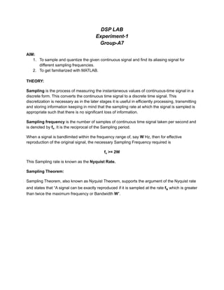
  • 1. DSP LAB Experiment-1 Group-A7 AIM: 1. To sample and quantize the given continuous signal and find its aliasing signal for different sampling frequencies. 2. To get familiarized with MATLAB. THEORY: Sampling is the process of measuring the instantaneous values of continuous-time signal in a discrete form. This converts the continuous time signal to a discrete time signal. This discretization is necessary as in the later stages it is useful in efficiently processing, transmitting and storing information keeping in mind that the sampling rate at which the signal is sampled is appropriate such that there is no significant loss of information. Sampling frequency is the number of samples of continuous time signal taken per second and is denoted by fs. It is the reciprocal of the Sampling period. When a signal is bandlimited within the frequency range of, say W Hz, then for effective reproduction of the original signal, the necessary Sampling Frequency required is fs >= 2W This Sampling rate is known as the Nyquist Rate. Sampling Theorem: Sampling Theorem, also known as Nyquist Theorem, supports the argument of the Nyquist rate and states that “A signal can be exactly reproduced if it is sampled at the rate fs which is greater than twice the maximum frequency or Bandwidth W”.
  • 2. Let’s assume a Bandlimited x(t) which has Fourier Transform X(w) as shown below. If a signal is sampled at a rate greater than 2W in the frequency domain, then the resultant Fourier Transform of the sampled signal is produced in such a manner that there will be gap in between two adjacent X(w) and the signal will be recoverable easily as shown below. If the signal is sampled at a rate of 2W, then the adjacent samples will be just touching at the ends.
  • 3. If the signal is sampled at a rate less than 2W, then the adjacent samples will be overlapping which leads to loss of information. This unwanted phenomenon of overlapping is called as aliasing. Corrective measures can be taken for prevention of aliasing such as, · A Low pass Anti-aliasing filter can be employed, before sampling to eliminate the high frequency components. · The input signal can be sampled at a rate higher than the Nyquist frequency for proper retrieval of the information. The choice of having Sampling rate greater than that of Nyquist rate also helps in easier design of the reconstruction filter at the receiver. Quantization Quantization refers to the process of digitizing the discrete time signal (which is sampled from continuous time signal) to a limited number of points by rounding off the samples to the nearest digital value.
  • 4. Both Sampling and Quantization result in loss of information but an appropriate signal can be reconstructed by taking proper Sampling rate for Sampling and Quantization levels for Quantization. The discrete amplitudes of the quantized output are known as representation levels and the space between two adjacent representation levels is known as step-size or quantum. Code and Output: Part-A: 1.Sample the sinusoid xa = 3sin(2πFt), where F = 2kHz at two different sampling frequencies, Fs1 = 3kHz and Fs2 = 5kHz and plot the sampled signals. Use functions `stem' and `subplot'. Code: F=2000; fs1=3000; fs2=5000; t=0:1/200000:0.001; %Defining f,fs1,fs2 and t x=sin(2*pi*F*t); %continuous time signal x(t) subplot(311);
  • 5. plot(t,x); %Plotting continuous signal title("X vs t"); n=0:1:10*fs1/F; Y=sin(2*pi*F/fs1*n);%Sampled signal x(nTs) at frequency fs1=3000 subplot(312); stem(n,Y); %Plotting discrete time signal using stem title("Xn vs n(fs=3000)"); n=0:1:10*fs2/F; Y=sin(2*pi*F/fs2*n);%Sampled signal x(nTs) at frequency fs1=3000 subplot(313); stem(n,Y); title("Xn vs n(fs=5000)"); Output:
  • 6. 2. Plot the sampled signals over the original continuous-time signal. (Use `hold')(All signals in MATLAB are discrete-time, but they will look like continuous-time signals if the sampling rate is much higher than the Nyquist rate). Code: F = 2000; T = 1/F; Fs1 = 3000; Fs2 = 5000; %Defining F,Fs1,Fs2 and T dt1 = 1/Fs1; dt2 = 1/Fs2; t = 0:0.00001:4*T; t1 = 0:dt1:4*T; t2 = 0:dt2:4*T; x_a = 3*sin(2*pi*F*t); %continuous time signal x(t) x_a1 = 3*sin(2*pi*F*t1); %Sampled signal x(nTs) at frequency fs1=3000 x_a2 = 3*sin(2*pi*F*t2); %Sampled signal x(nTs) at frequency fs2=5000 subplot(2,1,1); stem(t1,x_a1); %Plotting sampled signal using stem title('Sampled with Fs1'); hold on; %using hold function to plot two graphs on the same plot figure plot(t,x_a); hold off; subplot(2,1,2); stem(t2,x_a2); %Plotting sampled signal using stem title('Sampled with Fs2'); hold on;
  • 7. plot(t,x_a); hold off; Output: 3. Express the above as a 3-bit digital signal. Sample at Fs3 = 15kHz. Plot the sampled curve (use `stem') and over it plot the original curve. Code: fs=15000; f=2000; t=0:1/200000:1/500; nTs=0:1/fs:1/500; x=sin(2*pi*f*t); %continuous time signal y=sin(2*pi*f*nTs); %sampled signal x(nTs) N_samples=length(y); %creating array of length Yq=zeros(1,N_samples); %of sampled signal del=2/2^(3); %finding delta value for quantising
  • 8. disp(del); %displaying delta value V_max=1-del/2; %calculating max voltage level corresponding to 111 V_min=-1+del/2; %calculating min voltage level corresponding to 000 for i=V_min:del:V_max %doing a nested for loop to compare each for j=1:N_samples %sampled value with each voltage value corresponding if(((i-del/2)<y(j))&&(y(j)<(i+del/2)))%to each 3 bit binary value Yq(j)=i; end end end plot(t,x); %plotting the continuous time signal hold on; stem(nTs,Yq); %plotting the quantised sampled signal using stem hold off; Output:
  • 9. Part B 1. Consider an analog signal x(t) consisting of three sinusoids of frequencies of 1 kHz, 4 kHz, and 6 kHz: x(t)= cos(2000πt)+ cos(8000πt)+ cos(12000πt) Show that if this signal is sampled at a rate of Fs = 5 kHz, it will be aliased with the following signal, in the sense that their sample values will be the same: xa(t)= 3 cos(2000πt) On the same graph, plot the two signals x(t) and xa(t) versus t in the range 0 to 2 milli sec. To this plot, add the time samples x[n] (x(nTs)) and verify that x(t) and xa(t) intersect precisely at these samples. Given signal, x(t) = cos(2000πt)+ cos(8000πt)+ cos(12000πt) After sampling with sampling rate 5kHz, x(nTs) = cos(2πn/5)+ cos(8πn/5)+ cos(12π/5) It can be rearranged and written as, x[n] = cos(2πn/5)+ cos((2π-2π/5)n)+ cos((2π+2π/5)n) x[n] = 3cos(2πn/5) Hence the aliasing signal will be, xa(t) = 3cos(2000πt) Code f1 = 1000; f2 = 4000; f3 = 6000; %signal frequencies t = 0:0.000001:0.002; %defining tmin, tmax and the time step for continuous wave x_t = cos(2*pi*f1*t) + cos(2*pi*f2*t) + cos(2*pi*f3*t); % x(t) Fs = 5000; %sampling frequency dt = 1/Fs; ts = 0:dt:0.002; %defining the sampling instances x_ts = cos(2*pi*f1*ts) + cos(2*pi*f2*ts) + cos(2*pi*f3*ts); %sampled wave x_a = 3*cos(2000*pi*t); %Aliasing signal figure(3)
  • 10. subplot(3,1,1) plot(t, x_t) title("Analog signal x(t)") %plotting the analog signal subplot(3,1,2) stem(ts, x_ts) ylabel("Amplitude") title("Sampled signal x(nT)") %plotting the sampled signal subplot(3,1,3) stem(ts, x_ts) xlabel("time") title("Sampled signal x[n] intersecting with xa and x") hold on plot(t,x_a) plot(t,x_t,"r--") hold off % plotting the original, sampled and aliasing graphs Output
  • 11. 2. Repeat 1 with Fs = 10kHz. Determine the signal xa(t) with which x(t) is aliased. Given signal, x(t) = cos(2000πt)+ cos(8000πt)+ cos(12000πt) After sampling with sampling rate 10kHz, x(nTs) = cos(2πn/10)+ cos(8πn/10)+ cos(12π/10) It can be rearranged and written as, x[n] = cos(2πn/10)+ cos(8πn/10)+ cos((2π-8π/10)n) x[n] = cos(2πn/10) + 2cos(8πn/10) Hence the aliasing signal will be, xa(t) = cos(2000πt) + 2cos(8000πt) Code f1 = 1000; f2 = 4000; f3 = 6000;%signal frequencies t = 0:0.000001:0.002; %defining tmin, tmax and the time step for continuous wave x_t = cos(2*pi*f1*t) + cos(2*pi*f2*t) + cos(2*pi*f3*t) ; % x(t) Fs = 10000; %sampling frequency dt = 1/Fs; ts = 0:dt:0.002; %defining the sampling instances x_ts = cos(2*pi*f1*ts) + cos(2*pi*f2*ts) + cos(2*pi*f3*ts); %sampled wave x_a = cos(2000*pi*t) + 2*cos(8000*pi*t); %Aliasing signal figure(4) subplot(3,1,1) plot(t, x_t) title("Analog signal x(t)") %plotting the analog signal subplot(3,1,2) stem(ts, x_ts) ylabel("Amplitude") title("Sampled signal x(nT)") %plotting the sampled signal subplot(3,1,3) stem(ts, x_ts)
  • 12. xlabel("time") title("Sampled signal x[n] intersecting with xa and x") hold on plot(t,x_a) plot(t,x_t,"r--") hold off % plotting the original, sampled and aliasing graphs 3. Determine the sampling rate at which you can avoid the aliasing problem. To avoid aliasing we should have the sampling frequency should satisfy nyquist criteria. The maximum frequency of the given signal is 6000Hz. Hence the sampling frequency should be at least 12000 Hz. Code f1 = 1000; f2 = 4000; f3 = 6000;%signal frequencies
  • 13. t = 0:0.000001:0.002; %defining tmin, tmax and the time step for continuous wave x_t = cos(2*pi*f1*t) + cos(2*pi*f2*t) + cos(2*pi*f3*t) ; % x(t) Fs = 12000; %sampling frequency dt = 1/Fs; ts = 0:dt:0.002; %defining the sampling instances x_ts = cos(2*pi*f1*ts) + cos(2*pi*f2*ts) + cos(2*pi*f3*ts); %sampled wave figure(6) subplot(2,1,1) plot(t, x_t) title("Analog signal x(t)") %plotting the analog signal subplot(2,1,2) stem(ts, x_ts) ylabel("Amplitude") title("Sampled signal x(nT)") %plotting the sampled signal
  • 14. Conclusion: ● Successfully simulated the Continuous time signal and its corresponding discrete time signals sampled at various sampling frequencies. Quantization of the same discrete time signal was simulated as a 3-bit digital system. ● Aliasing effect was analyzed when the sampling rate is below the Nyquist rate and was corrected appropriately by using the Sampling Theorem. The results were verified by simulating in MATLAB. Group Members Kesavarapu Sai Sumanth B190669EC Kananathan Kajaruban B190519EC Guguloth Pramod B190776EC Laxman Satyappa Chinnannavar B190741EC Abel Antony Mathew B190660EC
  • 15. DSP Lab Experiment 2 Group A7 January 17th 2022 Kesavarapu Sai Sumanth (B190669EC), saisumanth b190669ec@nitc.ac.in Kananathan Kajaruban (B190519EC), kananathan b190519ec@nitc.ac.in Guguloth Pramod (B190776EC), pramod b190776ec@nitc.ac.in Laxman Satyappa Chinnannavar (B190741EC), laxman b190741ec@nitc.ac.in Abel Antony Mathew (B190660EC), abel b190660ec@nitc.ac.in 1 Introduction In todays world, electrical circuits consisting of resistors, inductors, capacitors and transistors are an important aspect of our everyday life. Electrical circuits are a type of system known as linear time invariant system. A system is said to be linear when it satisfies the condition of additivity and homogeneity. For the system to be time invariant the behaviour of the system should be independent of the time when the input is applied, i.e the output does not depend on the time of application of the input. The relation between the three signals;the input(x[n]), impulse response(h[n]) and output(y[n]) is given by: y[n] = x[n] ∗ h[n] The ’*’ operation is called convolution. In mathematics (in particular, func- tional analysis), convolution is a mathematical operation on two functions (x and h) that produces a third function (y) that expresses how the shape of one is modified by the other. It is the single most important function in Digital Signal Processing. In this experiment we are going: 1. To plot a signal and obtain it’s linear convolution with the given impulse response. 2. To find step response of an LTI system using the given impulse response and to compute the response to a rectangular pulse, exponential signal and a sinusoidal signal. 3. To show stable and unstable conditions for the given LTI system. 4. To show the stability condition change using pole-zero plot for the given system. 5. To apply a filter to an image by implementing circular convolution using 1
  • 16. overlap add method and overlap save method. 2 Background Topics 2.1 Aliasing In signal processing and related disciplines, aliasing is an effect that causes dif- ferent signals to become indistinguishable when sampled. It is an error created in a digital image that usually appears as a jagged outline 2.2 Impulse & Step input An impulse input is a very high pulse applied to a system over a very short time, i.e. the magnitude of the input approaches infinity while the time approaches zero. Step response is the time behaviour of the outputs of a general system when its inputs change from zero to one in a very short time. 2.3 Even & Odd signals To discern even or odd signals, waveform symmetry must be observed. Even signals are symmetric around vertical axis, and Odd signals are symmetric about origin. 3 Questions 3.1 Problem Statement Q1. Plot signal x (n) =[1 1 1 0 1 2 3 4], where x(0) = 0; (a) Plot x(n) and x(n + 2). (b) Obtain linear convolution with system h (n) =[1 2 1 -1], h(0) = 2; Show the output. (c) Verify your result with that obtained from in-built function in MATLAB. 3.1.1 Theory Convolution Convolution is a mathematical way of combining two signals to form a third signal. It is the single most important technique in Digital Signal Processing. The term convolution refers to both the result function and to the process of computing it. It is defined as the integral of the product of the two functions after one is reversed and shifted. And the integral is evaluated for all values of shift, producing the convolution function. 2
  • 17. Linear convolution Linear convolution is a mathematical operation done to calculate the output of any Linear-Time Invariant (LTI) system given its input and impulse response. We can represent Linear Convolution as y[n] = x[n] h[n] Here, y(n) is the out- put (also known as convolution sum), x(n) is the input signal, and h(n) is the impulse response of the LTI system. y[n] = ∞ X n=−∞ x[n0]h[n − n0] Linear convolution may or may not result in a periodic output signal. 3.1.2 Code x n = [1 1 1 0 1 2 3 4 ] ; n = −3:4; figure (1) subplot (3 ,1 ,1) stem(n , x n ) t i t l e (”x [ n ] ” ) n1 = −n ; subplot (3 ,1 ,2) stem(n1 , x n ) t i t l e (”x[−n ] ” ) ylabel (” Amplitude ”) n2 = −n+2; subplot (3 ,1 ,3) stem(n2 , x n ) t i t l e (”x[−n+2]”) xlabel (”n”) h n = [1 2 1 −1]; n h = −1:2; n y = −4:6; Y = convolve ( x n , h n ) ; figure (2) stem( n y ,Y) t i t l e (” Convolution using written function ”) xlabel (”n”) ylabel (”y [ n ] ” ) L = length ( x n ) ; 3
  • 18. M = length ( h n ) ; N = L + M − 1; z = zeros (1 ,N) ; z = conv( x n , h n ) ; figure (3) stem( n y , z ) t i t l e (” Convolution using i n b u i l t function ”) xlabel (”n”) ylabel (”y [ n ] ” ) function [Y] = convolve ( x n , h n ) L = length ( x n ) ; M = length ( h n ) ; N = L + M − 1; Y = zeros (1 ,N) ; X = [ x n , zeros (1 ,M) ] ; H = [ h n , zeros (1 ,L ) ] ; for i =1:N for j =1: i Y( i ) = Y( i ) + X( j )∗H( i−j +1); end end end 3.1.3 Output The output for the corresponding code is shown below in Figures 1, 2 and 3. 3.1.4 Inference Here we have performed reversal and shifting operation on discrete time signal, and we can observe that the output matches the theoretical approach. We have also performed convolution with the system h[n] using mathematical approach in the algorithm. Also we have verified our results using the inbuilt function. 4
  • 19. Figure 1: Reversal and shifting operation. Figure 2: Convolution using written function. 5
  • 20. Figure 3: Convolution using inbuilt function.. 3.2 Problem Statement Q2. Use the above program function (you wrote) to find the step response of an LTI system given the impulse response. (Take h[n] = 1, 2, 3, 4). Also compute the response of the same system to a rectangular pulse, exponential signal and a sinusoidal signal. 3.2.1 Theory LTI System Linear Time-Invariant systems are a class of systems used in signals and systems that are both linear and time invariant. Linear systems are systems whose outputs for a linear combination of inputs are the same as a linear combination of individual responses to those inputs. LTI systems play a significant role in digital communication system analysis and design, as an LTI system can be easily characterized either in the time domain using the system impulse response or in the frequency domain using the system transfer function. 6
  • 21. 3.2.2 Code h = [1 2 3 4 ] ; figure (1) stem(h) t i t l e (” Impulse Response ”) xlabel (”n”) ylabel (”h [ n ] ” ) u n = ones ( 1 , 2 0 ) ; n = 0 : 1 9 ; q = convolve ( u n , h ) ; figure (2) stem(n , u n ) t i t l e (” Unit step input ”) xlabel (”n”) ylabel (”u [ n ] ” ) figure (3) stem(q) t i t l e (” Covolution with unit step input ”) xlabel (”n”) ylabel (” Amplitude ”) rect = [0 0 0 1 1 1 1 1 0 0 0 ] ; n = −5:5; p = convolve ( rect , h ) ; figure (4) stem(n , rect ) t i t l e (” Rectangular input ”) xlabel (”n”) ylabel (” rect [ n ] ” ) figure (5) stem(p) t i t l e (” Covolution with rectangular wave”) xlabel (”n”) ylabel (” Amplitude ”) n = 0 : 2 0 ; x2 = exp(n ) ; d = conv(x2 , h ) ; figure (6) stem( x2 ) t i t l e (” Exponential input ”) xlabel (”n”) ylabel (”exp [ n ] ” ) figure (7) 7
  • 22. stem(d) t i t l e (” Covolution with exponential wave”) xlabel (”n”) ylabel (” Amplitude ”) x1 = cos (0.08∗ pi∗n ) ; f = convolve (x1 , h ) ; figure (8) stem( x1 ) t i t l e (” Sinusoidal input ”) xlabel (”n”) ylabel (”x [ n ] ” ) figure (9) stem( f ) t i t l e (” Covolution with s i n u s o i d a l wave”) xlabel (”n”) ylabel (” Amplitude ”) function [Y] = convolve ( x n , h n ) L = length ( x n ) ; M = length ( h n ) ; N = L + M − 1; Y = zeros (1 ,N) ; X = [ x n , zeros (1 ,M) ] ; H = [ h n , zeros (1 ,L ) ] ; for i =1:N for j =1: i Y( i ) = Y( i ) + X( j )∗H( i−j +1); end end end 3.2.3 Output 8
  • 23. Figure 4: Impulse Response of the system. Figure 5: Output for corresponding Unit Step input 9
  • 24. Figure 6: Output for corresponding Rectangular wave Figure 7: Output for corresponding Exponential input Figure 8: Output for corresponding Sinusoidal input 10
  • 25. 3.3 Problem Statement Q3. Show stable and unstable conditions for the linear time invariant system: h(n) = an u(n) Use the convolution function you wrote appropriately to show this outcome. (a) Obtain pole-zero plot for both conditions. (Vary location of the pole, one at ROC limit, one outside and one inside and observe the system response over time). 3.3.1 Theory BIBO stability condition A discrete-time system is BIBO stable if and only if the output sequence y[n] remains bounded for all bounded input sequence x[n] An LTI discrete-time system is BIBO stable if and only if its response sequence h[n] is absolutely summable, i.e. S = ∞ X n=−∞ |h[n]| < ∞ Analysing Stabilty of System using Z transform and ROC We can determine whether a system is stable or not using the position of poles of the system transfer function in the Z plane. In order for the system to be stable, the unit circle should lie within the Region of Covergence(ROC). For right sided sequence the ROC will be outward and vice versa. The Z-transform of the system response h[n] is given by, 11
  • 26. H(Z) = ∞ X n=−∞ h[n]Z−n In the given problem, h[n] = an u[n] Therefore using the above equation we obtain the Z-transform, H(Z) = ∞ X n=−∞ h[n]Z−n = 1/1 − aZ−1 Here since u[n] is a right sided sequence the ROC will be outwards from the pole circle. And therefore all poles must be contained within the unit circle,i.e |z| = |a| < 1 3.3.2 Code clc ; x = [−1 −2 1 3 2 4 1 ] ; nmax = 20; a = 0 . 5 0 ; %or 1.5 for unstable condition n = 0:nmax ; h = [ ] ; for i =1:nmax t = aˆ i ; h =[h t ] ; end out = convolve (x , h ) ; figure (1) subplot (221) stem(x ) ; t i t l e (” Input ”) ylabel (” Amplitude ”) xlabel (”n”) subplot (222) stem(h ) ; grid on t i t l e (” Impulse Response ( a = 0.5 ( <1))”) ylabel (” Amplitude ”) 12
  • 27. xlabel (”n”) subplot (223) stem( out ) ; grid on t i t l e (” Output ”) ylabel (” Amplitude ”) y = conv(x , h ) ; subplot (224) stem(y ) ; t i t l e (” Output using i n b u i l t function ”) xlabel (”n”) ylabel (” Amplitude ”) figure (2) subplot (211) a =1.5; zplane (0 , a ) t i t l e (” Unstable condition ( Outside ROC l i m i t ) (a>1)”) subplot (212) h = [ ] ; for i =1:nmax t = aˆ i ; h =[h t ] ; end out = convolve (x , h ) ; stem( out ) t i t l e (” System response for the given x [ n ] ” ) ylabel (” Amplitude ”) xlabel (”n”) figure (3) subplot (211) a=1; zplane (0 , a ) t i t l e (”At ROC l i m i t ( a=1)”) subplot (212) h = [ ] ; for i =1:nmax t = aˆ i ; h =[h t ] ; end out = convolve (x , h ) ; 13
  • 28. stem( out ) t i t l e (” System response for the given x [ n ] ” ) ylabel (” Amplitude ”) xlabel (”n”) figure (4) subplot (211) a =0.5; zplane (0 , a ) t i t l e (” Stable condition ( Inside ROC l i m i t ) (a<1)”) subplot (212) h = [ ] ; for i =1:nmax t = aˆ i ; h =[h t ] ; end out = convolve (x , h ) ; stem( out ) t i t l e (” System response for the given x [ n ] ” ) ylabel (” Amplitude ”) xlabel (”n”) function [Y] = convolve ( x n , h n ) L = length ( x n ) ; M = length ( h n ) ; N = L + M − 1; Y = zeros (1 ,N) ; X = [ x n , zeros (1 ,M) ] ; H = [ h n , zeros (1 ,L ) ] ; for i =1:N for j =1: i Y( i ) = Y( i ) + X( j )∗H( i−j +1); end end end 3.3.3 Output Output for the corresponding code is shown in the Figures 9,10,11,12 and 13. 14
  • 29. Figure 9: Output for Stable System. Figure 10: Output for Unstable System. 15
  • 30. Figure 11: Pole Zero plot and System Response for Unstable System (a>1). Figure 12: Pole Zero plot and System Response for Unstable System (a=1). 16
  • 31. Figure 13: Pole Zero plot and System Response for Stable System (a<1). 3.3.4 Inference Here we have assumed an input x = [-1 -2 1 3 2 4 1] (bounded input) and we have convoluted this with our impulse response to view the output for two different conditions. From the plots we can observe that when a=0.5, the output we get is absolutely summable and when a = 1.5, the output we get is in the range of 104 , which cannot be viewed as a bounded output. Hence we can conclude that when a<1 the system is stable and when a>1 the system is unstable. 3.4 Problem Statement Q4. Can you show the stability condition change using pole-zero plot, if we were dealing with the system h(0) = an n = 0 bn n 0 ,show the results as a plot. (Vary location of the pole, one at ROC limits, outside (two cases) and one inside and observe the system response over time). 17
  • 32. 3.4.1 Theory Analysing the impulse response of the given system Given the impulse response, h[n] = an u[n] + b−n u[−n − 1] The Z-transform of h[n] is given by, H(Z) = 1/(1 − aZ−1 ) + 1/(bZ−1 − 1) The ROC of the above system is, |a| |z| |b| So in order for the unit circle to be included in the ROC, |a| 1 |b| 3.4.2 Code Listing 1: Stability conditions using pole-zero plot clc x = [−1 −2 1 3 2 4 1 ] ; figure (1) subplot (211) a = 1 . 5 ; b = 2; zplane ( 0 , [ a ; b ] ) t i t l e (” Unstable condition ( Outside ROC l i m i t ) (a1 or b1)”) subplot (212) h = t r a n s f e r f u n c (a , b ) ; out = convolve (x , h ) ; stem( out ) t i t l e (” System response for the given x [ n ] ” ) ylabel (” Amplitude ”) xlabel (”n”) figure (2) subplot (211) a = 0 . 2 ; b = 0 . 5 ; zplane ( 0 , [ a ; b ] ) t i t l e (” Unstable condition ( Outside ROC l i m i t ) (a1 or b1)”) 18
  • 33. subplot (212) h = t r a n s f e r f u n c (a , b ) ; out = convolve (x , h ) ; stem( out ) t i t l e (” System response for the given x [ n ] ” ) ylabel (” Amplitude ”) xlabel (”n”) figure (3) subplot (211) a=1; b=1; zplane ( 0 , [ a ; b ] ) t i t l e (”At ROC l i m i t ( a=1 and b=1)”) subplot (212) h = t r a n s f e r f u n c (a , b ) ; out = convolve (x , h ) ; stem( out ) t i t l e (” System response for the given x [ n ] ” ) ylabel (” Amplitude ”) xlabel (”n”) figure (4) subplot (211) a = 0 . 5 ; b = 2 . 5 ; zplane ( 0 , [ a ; b ] ) t i t l e (” Stable condition ( Inside ROC l i m i t ) (a1 and b1)”) subplot (212) h = t r a n s f e r f u n c (a , b ) ; out = convolve (x , h ) ; stem( out ) t i t l e (” System response for the given x [ n ] ” ) ylabel (” Amplitude ”) xlabel (”n”) function [Y] = convolve ( x n , h n ) L = length ( x n ) ; M = length ( h n ) ; N = L + M − 1; Y = zeros (1 ,N) ; 19
  • 34. X = [ x n , zeros (1 ,M) ] ; H = [ h n , zeros (1 ,L ) ] ; for i =1:N for j =1: i Y( i ) = Y( i ) + X( j )∗H( i−j +1); end end end function [ h ] = t r a n s f e r f u n c (a , b) h = zeros (1 , 201); i = 1; for n = −10:0.1: −0.1 h( i ) = b .ˆ n ; i = i +1; end for n = 0 : 0 . 1 : 1 0 h( i ) = a .ˆ n ; i = i +1; end end 20
  • 35. 3.4.3 Output In this case we took a = 1.5 and b = 2, Here a 1 causes the instability condition As we can see in the above plot, the system response for x[n], the amplitude of the output almost reaches 600 which shows that the output is unbounded. 21
  • 36. In this case we took a = 0.2 and b = 0.5, Here b 1 causes the instability condition. As we can see in the above plot, the system response for x[n], the amplitude of the output almost reaches 7500 which shows that the output is unbounded. 22
  • 37. In this case we took a = b = 1 i.e both the poles are on the unit circle ROC. As we can see in the above plot, the system response for x[n], the maximum amplitude of the output is only 11 which shows that the output is stable and bounded 23
  • 38. In this case we took a = 0.5 and b = 2.5. As we can see in the above plot, the system response for x[n], the maximum amplitude of the output is only 8 which again shows that the output is stable and bounded. 24
  • 39. 3.5 Problem Statement Q5. Read an image and resize it to 32x32. Then convert it into a row vector of length 1x1024. Apply the filter given by h[n]= 1/3 1/3 1/3 on the long row vector by making use of overlap-add and overlap-save approach. Rearrange the output sequence to image format. What are the observations? 3.5.1 Theory Circular Convolution Circular convolution is essentially the same process as linear convolution. Just like linear convolution, it involves the operation of folding a sequence, shifting it, multiplying it with another sequence, and sum- ming the resulting products. However, in circular convolution, the signals are all periodic. Thus, the shifting can be thought of as actually being a rotation. Since the values keep repeating because of the periodicity. Hence, it is known as circular convolution. We can represent N point Circular Convolution as: y[n] = N+1 X n=−0 x[n0]h[(n − n0)N ] Overlap Add method The overlap-add procedure cuts the signal up into equal length segments with no overlap. Then takes the Linear convolution of the segments with the impulse response. Part of the convolution result cor- responds to the circular convolution. The tails that do not correspond to the circular convolution are added to the adjoining tail of the previous and sub- sequent sequence. This addition results in the aliasing that occurs in circular convolution. Overlap Save method The overlap-save algorithm filters the input signal in the frequency domain. The input is divided into overlapping blocks which are circularly convoluted with the FIR filter coefficients. 3.5.2 Code Listing 2: Convolution using overlap and add method I= imread (” pic1 . png ” ) ; K = rgb2gray ( I ) ; figure ( 1 ) ; imshow (K) ; 25
  • 40. J = K( : ) ; J = J ’ ; hn = [1/3 ,1/3 ,1/3]; M = 3; N= 2ˆM; L = N− M+1; J = [ J zeros ( 1 , 2 ) ] ; hn pad = [ hn zeros (1 ,L−1)]; over add = zeros (1 ,1026); c c i r c 1 = zeros ( 1 , 8 ) ; c c i r c 2 = zeros ( 1 , 8 ) ; for i = 1 : ( length (J)/L) xt1 = J(L∗( i −1) + 1:L∗( i −1) + L ) ; xt1 = [ xt1 zeros (1 ,M−1)]; c c i r c 1 = circ conv ( xt1 , hn pad ) ; for j =1:8 c c i r c 1 (1 , j ) = uint8 ( c c i r c 1 (1 , j ) ) ; end i f i==1 over add ( 1 :N− M+1) = c c i r c 1 ( 1 :N − M +1); continue ; else over add (L∗( i −1)+1:L∗( i −1)+2) = c c i r c 2 (N−1:N) + c c i r c 1 ( 1 : 2 ) ; over add (L∗( i −1) + 3:L∗( i −1) + 6) = c c i r c 1 ( 3 : 6 ) ; end c c i r c 2 = c c i r c 1 ; end new over add = over add ( 1 : 1 0 2 4 ) ; f i n a l a n s = uint8 ( zeros (1 ,1024)); for i =1:1024 f i n a l a n s (1 , i ) = uint8 ( new over add (1 , i ) ) ; end f i n a l a n s = reshape ( f i n a l a n s ,32 , [ ] ) ; figure ( 2 ) ; imshow ( f i n a l a n s ) function [Y] = circ conv (x , h) nx= length (x ) ; Y = zeros (1 , nx ) ; for i =1:nx for j =1:nx ind = mod(( i+j −2) ,nx)+1; 26
  • 41. Y( ind ) = Y( ind ) + x( i )∗h( j ) ; end end end Listing 3: Convolution using overlap and save method clc I= imread (” pic1 . png ” ) ; K = rgb2gray ( I ) ; figure ( 1 ) ; imshow (K) ; J = K( : ) ; J = J ’ ; hn = [1/3 ,1/3 ,1/3]; M = 3; N= 2ˆM; L = N− M+1; J len = length (J ) ; hn pad = [ hn zeros (1 ,L−1)]; over save = zeros (1 ,1024); c c i r c 1 = zeros ( 1 , 8 ) ; for i = 1: J len /L i f i == 1 xt1 = [ zeros (1 ,M−1) J ( 1 : 6 ) ] ; else xt1 = J(L∗( i −1) − 1: L∗( i −1) + 6 ) ; end c c i r c 1 = circ conv ( hn pad , xt1 ) ; over save (L∗( i −1)+1:L∗( i )) = c c i r c 1 ( 3 : 8 ) ; end whos over save f i n a l a n s = uint8 ( zeros (1 ,1024)); for i =1:1024 f i n a l a n s (1 , i ) = uint8 ( over save (1 , i ) ) ; end f i n a l a n s = reshape ( f i n a l a n s , 32 , [ ] ) ; figure ( 2 ) ; imshow ( f i n a l a n s ) ; function [Y] = circ conv (h , x) nx= length (x ) ; Y = zeros (1 , nx ) ; 27
  • 42. for i =1:nx for j =1:nx ind = mod(( i+j −2) ,nx)+1; Y( ind ) = Y( ind ) + x( i )∗h( j ) ; end end end 3.5.3 Output Figure 14: Input Picture 28
  • 43. Figure 15: Output Image after performing overlap and add convolution Figure 16: Output Image after performing overlap and save convolution 29
  • 44. 3.5.4 Inference After performing the linear convolution of the converted image matrix with the filter using the 2 methods, we observed that the outputs of both the methods were similar and a little blurred as compared to the original image but retaining some characteristics of the original image. Properties like the overall shape and color were still same as the original. From observation we also found that the neighbouring pixels of a pixel affected it to change the color and hence the blurred image is formed. 4 Outcomes and Critical Analysis of the exper- iment • Obtained a proper understanding of linear convolution and circular con- volution and its implementation in the MATLAB • Implemented the code for detecting the stability of LTI systems based on the transfer function. Also we verified the stability conditions of the pole zero plots by plotting the system response with a particular input discrete time signal. Observed that whenever the transfer function was unstable, the BIBO stability criteria was not achieved as for a bounded input the outoput was unbounded. And when the transfer function was stable, the BIBO stability criteria was achieved. • Explored different methods to evaluate the linear convolution using over- lap and add method and overlap and save method. Expanded our knowl- edge of array manipulation in MATLAB. Also obtained the knowledge of different functions used in digital image processing like imread, rgb2gray, padding, etc • Obtained a basic understanding in digital image processing. Understood what are filters used for in image processing and how to apply the filter to an image. 30
  • 45. DSP Lab Experiment 3 Group A7 February 6th 2022 Kesavarapu Sai Sumanth (B190669EC), saisumanth b190669ec@nitc.ac.in Kananathan Kajaruban (B190519EC), kananathan b190519ec@nitc.ac.in Guguloth Pramod (B190776EC), pramod b190776ec@nitc.ac.in Laxman Satyappa Chinnannavar (B190741EC), laxman b190741ec@nitc.ac.in Abel Antony Mathew (B190660EC), abel b190660ec@nitc.ac.in 1 Introduction In this experiment, we are going: 1. To plot the frequency spectrum, magnitude spectrum, and sample spectrum for the given sinusoidal signal. 2. To obtain DFT of the sampled signal and compare to the sample spectrum. 3. To multiply two DFTs and show it’s relation to circular convolution. 4. Implement the radix-2 FFT algorithm to compute the N-point DFT of a sequence. 5. To test the FFT program by computing DFT for a. Rectangular pulse b. Sinusoidal signal c. Unit impulse and to reconstruct the signals back from the spectrum using the IDFT program and to observe the effect of zero padding using different number of samples, while plotting the spectrum. 2 Questions Part A 2.1 Problem Statement Q1. Sample the sinusoid xa = 3sin(2πFt), where F = 2kHz at sampling frequency, Fs = 8kHz and plot the sampled signal. (a) Plot the frequency spectrum of the above signal. (b) The magnitude spectrum is sampled at frequencies wk = (2πk/N)∗k ; k = 0, ....., N − 1 . Plot sampled spectrum for N = 5, N = 50 and N 1
  • 46. =100. (c) Obtain DFT of the sampled signal using X(k) = 1/N PN−1 n=0 x(n)e−j2πkn/N . Plot for N = 5, 50, 100 and compare to output of part b. 2.1.1 Theory DTFT The Discrete Time Fourier Transform (DTFT) is a form of Fourier analysis that is used to analyze the discrete time non-periodic signals. The DTFT is a frequency-domain representation for a wide range of both finite and infinite-length discrete-time signals x[n]. The DTFT of a sequence x[n] is a continuous function of frequency, -, and defined as X(eiw ) = ∞ X n=−∞ x[n]eiwn DFT The Discrete Fourier transform (DFT) converts a finite sequence of equally spaced samples of a function into a same-length sequence of equally-spaced samples of the discrete-time Fourier transform (DTFT), which is a complex- valued function of frequency. The Discrete Fourier transform transforms a sequence of N complex numbers, x[N] = x[0], x[1], ..., x[N − 1] into another sequence of complex numbers, X[k] = X[0], X[1], ..., X[N − 1], which is defined as Xk = N−1 X n=0 x[n]e−i2πkn/N 2.1.2 Code c l c ; c l e a r ; F=2000; Fs=8000; ts=1/Fs ; t =0:1/200000:4/2000; n=0:4∗Fs/F; x=3∗sin (2∗ pi ∗F∗ t ) ; x n=3∗sin (2∗ pi ∗F∗ ts ∗n ) ; subplot (311) plot ( t , x ) ; t i t l e ( ’X( t ) vs t ’ ) ; ylabel ( ’ x( t ) ’ ) ; xlabel ( ’ t ’ ) ; subplot (312); 2
  • 47. stem ( x n ) ; t i t l e ( ’X[ n ] vs n ’ ) ; ylabel ( ’X[ n ] ’ ) ; xlabel ( ’n ’ ) ; w=0:1/1000:2∗ pi ; x w=0; f or i=n x w=x w+x n ( i +1)∗(exp(− j ∗w) ) . ˆ i ; end ; y=abs ( x w ) ; subplot (313); plot (w, y ) ; t i t l e ( ’X[ Ω ] vs Ω ’ ) ; ylabel ( ’X[ Ω ] ’ ) ; xlabel ( ’Ω ’ ) ; f i g u r e ( 2 ) ; N=5; wk1=0:2∗ pi /N:2∗ pi ; x w=0; f or i=n x w=x w+x n ( i +1)∗(exp(− j ∗wk1 ) ) . ˆ i ; end ; y=abs ( x w ) ; subplot (311); stem (wk1 , y ) ; N=50; wk2=0:2∗ pi /N:2∗ pi ∗(N−1)/N; x w=0; f or i=n x w=x w+x n ( i +1)∗(exp(− j ∗wk2 ) ) . ˆ i ; end ; y=abs ( x w ) ; subplot (312); stem (wk2 , y ) ; N=100; wk3=0:2∗ pi /N:2∗ pi ∗(N−1)/N; x w=0; f or i=n x w=x w+x n ( i +1)∗(exp(− j ∗wk3 ) ) . ˆ i ; end ; y=abs ( x w ) ; 3
  • 48. subplot (313); stem (wk3 , y ) ; f i g u r e ( 3 ) ; N=5; n1=0:N−1; x n1=3∗sin (2∗ pi ∗F∗ ts ∗n1 ) ; disp ( x n1 ) ; k=0:N−1; x k =0; f or i =0:N−1 x k=x k+x n1 ( i +1)∗(exp(− j ∗2∗ pi /N∗k ) ) . ˆ i end ; y=1/N∗abs ( x k ) ; subplot (311); stem (k , y ) ; t i t l e ( ’X[ k ] vs k(N=5) ’); ylabel ( ’X[ k ] ’ ) ; xlabel ( ’ k ’ ) ; N=50; n1=0:N−1; x n1=3∗sin (2∗ pi ∗F∗ ts ∗n1 ) ; disp ( x n1 ) ; k=0:N−1; x k =0; f or i =0:N−1 x k=x k+x n1 ( i +1)∗(exp(− j ∗2∗ pi /N∗k ) ) . ˆ i end ; y=1/N∗abs ( x k ) ; subplot (312); stem (k , y ) ; t i t l e ( ’X[ k ] vs k(N=50) ’); ylabel ( ’X[ k ] ’ ) ; xlabel ( ’ k ’ ) ; N=100; n1=0:N−1; x n1=3∗sin (2∗ pi ∗F∗ ts ∗n1 ) ; disp ( x n1 ) ; k=0:N−1; x k =0; f or i =0:N−1 x k=x k+x n1 ( i +1)∗(exp(− j ∗2∗ pi /N∗k ) ) . ˆ i end ; y=1/N∗abs ( x k ) ; 4
  • 49. subplot (313); stem (k , y ) ; t i t l e ( ’X[ k ] vs k(N=100) ’); ylabel ( ’X[ k ] ’ ) ; xlabel ( ’ k ’ ) ; 2.1.3 Output Figure 1: plots of (i)x(t)vst (ii)x[n]vsn (iii)X(W)vsW. 5
  • 50. Figure 2: plots of X(W) vs Wk for (i)N=5 (ii)N=50 (iii)N=100. Figure 3: plots of DFT of x[n]: X(k) vs k for (i)N=5 (ii)N=50 (iii)N=100. 2.1.4 Inference Here we have plotted the frequency spectrum(X(W) vs W) of the initial sampled x[n]. Then we sampled the frequency spectrum at Wk=2πk/N: k=0,1,2,...N-1; for N=5,50,100. Then we calculated and plotted the N-point DFT of x[n] taking N=5,50,100 and compared it to the earlier sampled frequency spectrum. We can see that the plots are similar in shape but the peaks are sharper in the DFT 6
  • 51. plots due to taking N samples of x(t) for each DFT calculation. But this is not the case in the sampled frequency spectrum. So while taking the N-point DFT of x[n] we take that much more information by taking N number of samples of x(t), and that information is reflected in each DFT plot when compared to the frequency sampling plots. 2.2 Problem Statement Q2. Let x1(n) = [1 2 3] and x2(n) = [2 3], Obtain their respective 5-point DFTs, (a) Multiply the two DFTs and plot output. (b) Show relation to circular convolution using necessary plots. 2.2.1 Theory Circular Convolution The convolution theorem is a fundamental property of the Fourier transform. It is often stated as ”Convolution in time domain equals multiplication in frequency domain” or vice versa i.e., ”Multiplication in time equals convolution in the frequency domain”. Let x(t) and y(t) be two arbitrary signals. Then, we have X(f).Y (f) = F{x(t) ∗ y(t)} where F{x(t)} and X(f) denotes the Fourier transform of x(t). 2.2.2 Code x1 = [1 2 3 ] ; x2 = [2 3 ] ; N = 5; %zero pading x1 = [ x1 zeros (1 ,N−length ( x1 ) ) ] ; x2 = [ x2 zeros (1 ,N−length ( x2 ) ) ] ; X1 = d f t c a l c ( x1 ) ; X2 = d f t c a l c ( x2 ) ; Y = X1.∗X2; figure (1) stem(Y) t i t l e (” Multiplication of X1(k) and X2(k )”) xlabel (”k”) ylabel (”X1(k ) . X2(k )”) y = circ conv (x1 , x2 ) ; %c i r c u l a r convolution 7
  • 52. Yc = d f t c a l c (y ) ; figure (2) stem(Yc) t i t l e (”DFT of c i r c u l a r convolution of x1 and x2 ”) xlabel (”k”) ylabel (”DFT( x1∗x2 )”) function X = d f t c a l c (x) N = length (x ) ; X=zeros (1 ,N) ; for k=1:N for n=1:N X(k) = X(k) + x(n)∗exp(−2∗pi∗1 i ∗(n−1)∗(k−1)/N) ; end end end function [Y] = circ conv (h , x) nx= length (x ) ; Y = zeros (1 , nx ) ; for i =1:nx for j =1:nx ind = mod(( i+j −2) ,nx)+1; Y( ind ) = Y( ind ) + x( i )∗h( j ) ; end end end 8
  • 53. 2.2.3 Output Figure 4: Multiplication of two DFTs X1(k) and X2(k). Figure 5: DFT of circular convolution between x1(t) and x2(t). 9
  • 54. 2.2.4 Inference Here we have obtained 5 point DFT of x1(n) and x2(n) and performed multi- plication in frequency domain. Also we performed circular convolution of x1(n) and x2(n), obtained the DFT of the resulting convolution and plotted it. By observing the plot, we can conclude that Multiplication in Frequency Domain is equivalent to circular convolution in in Time Domain. Part B 2.3 Problem Statement Q.3 Implement the radix-2 FFT algorithm to compute the N-point DFT X[k] of a sequence x[n] of length N. Assume N = 2m . Make ‘N’ a variable. Modify to compute the N-point IDFT x[n] of X[k]. 2.3.1 Theory FFT The Fast Fourier Transform is a particularly efficient algorithm for performing Discrete Fourier Transforms of samples containing certain numbers of points. A discrete Fourier transform can be computed using an FFT, if the number of points N is a power of two. Fast Fourier transform algorithms generally fall into two classes: 1. Decimation in time 2. Decimation in frequency. Radix-2 FFT Decimation in Time The radix-2 decimation-in-time algorithm rearranges the Discrete Fourier trans- form (DFT) equation into two parts: A sum over the even-numbered discrete time indices n = [0, 2, 4, . . . , N - 2] and a sum over the odd-numbered indices n = [1, 3, 5, . . . , N - 1] Xk = DFTN/2[x[0], x[2], ...., x[N − 2]] + Wk N DFTN/2[x[1], x[3], ...., x[N − 1]] The above equation shows that the DFT frequency outputs X(k) can be com- puted as the sum of the outputs of two length-N2 DFTs, where the odd-indexed short DFT is multiplied by a twiddle factor term Wk N = e−i2πk/N This is called a decimation in time because the time samples are rearranged in alternating groups, and a radix-2 algorithm because there are two groups. Radix-2 FFT Decimation in Frequency The radix-2 decimation-in-frequency algorithm rearranges the Discrete Fourier transform (DFT) equation into two parts: Computation of the even-numbered discrete-frequency indices X(k) for k = 10
  • 55. [0, 2, 4, ..., N−2] and computation of the odd-numbered indices k = [1, 3, 5, ..., N− 1] X(2r) = DFTN/2[x(n) + x(n + N/2)] X(2r + 1) = DFTN/2[x(n) − x(n + N/2)]Wk N The above equations show both the even-indexed and odd-indexed frequency outputs of X(k) each computed by a length of N/2 DFT. The inputs to these DFTs are sums or differences of the first and second halves of the input sig- nal, respectively, where the input to the short DFT producing the odd-indexed frequencies is multiplied by a so-called twiddle factor term Wk N = e−i2πk/N . 2.3.2 Code m = 3; N=2ˆm; x = randi ( [ 1 , 1 0 ] , 1 ,N) ; X1 = f f t c a l c (x ) ; k = 0:N−1; figure (2) subplot (411) stem(k , abs( f f t (x ) ) ) t i t l e (”DFT using i n b u i l t function ”) xlabel (”k”) ylabel (”X[ k ] ” ) y = i d f t c a l c (X1/N) ; %i n t e p r e t i n g the input as X( k )/N to get the f i n a l answer subplot (412) stem(k , abs(X1)) t i t l e (”DFT using f f t algorithm ”) xlabel (”k”) ylabel (”X[ k ] ” ) subplot (413) stem(x) t i t l e (” Input x”) xlabel (”n”) ylabel (” Amplitude ”) subplot (414) stem(y) t i t l e (”y = IDFT[DFT(x ) ] ” ) xlabel (”n”) ylabel (” Amplitude ”) 11
  • 56. function X k = f f t c a l c (x) N = length (x ) ; i f N == 1 X k = x ; else g = x ( 1 : 2 :N) ; h = x ( 2 : 2 :N) ; G k = f f t c a l c ( g ) ; H = f f t c a l c (h ) ; k = ( 0 : (N/2 −1)) ’; W = (exp(−2∗pi∗1 i /N) ) . ˆ k ; H k = W.∗H; X k = [ G k+H k ; G k−H k ] ; end end function Y n = i d f t c a l c ( x k ) N = length ( x k ) ; i f N == 1 Y n = x k ; else g = x k ( 1 : 2 :N) ; h = x k ( 2 : 2 :N) ; G k = i d f t c a l c ( g ) ; H = i d f t c a l c (h ) ; k = ( 0 : (N/2 −1)) ’; W = (exp(2∗ pi∗1 i /N) ) . ˆ k ; H k = W.∗H; Y n = [ G k+H k ; G k−H k ] ; end end 12
  • 57. 2.3.3 Output Figure 6: DFT plotted using the inbuilt function in MATLAB. Figure 7: DFT plotted using the written function. 13
  • 58. Figure 8: Input signal x[n]. Figure 9: IDFT of the derived DFT of x[n]. 14
  • 59. 2.3.4 Inference Here we have implemented the FFT algorithm using recursive function. To verify its functionality, we took N number of random integers between 1 and 10 and calculated its DFT using both inbuilt and written function. By observing the obtained plots we can say that both are similar. Hence we can verify the functionality of the written FFT function. Also we have implemented the IDFT by modifying the same function. We modified it by changing the sign in twiddle factor and giving the input to the function as X[k]/N. From the above plots we can verify that the output of IDFT is same as the input sequence. 2.4 Problem Statement Q4. Test the FFT program by computing DFT for (a) A rectangular signal (b) sinusoidal signal (c) Unit impulse. Try to reconstruct the signals back from the spectrum using your IDFT program. Observe the effect of zero padding using different number of samples, while plotting the spectrum. 2.4.1 Theory In this section, we are implementing the DFT and IDFT functions for various signals like Rectangular, Sinusoidal and Unit Impulse. Also observe the changes caused due to zero padding. We are expecting no change in spectral resolution as sampling rate and No.of samples remain constant. Also we expect the IDFT of the DFT of signal gen- erates back the original signal which confirms that the functions written are correct. 2.4.2 Code clc ; clear al l ; n = 1 : 3 2 ; % Since n = 2ˆm; Here m = 5 %DFT and IDFT of Rectangular Signal rect = zeros ( 1 , 3 2 ) ; for i =10:20 rect ( i ) = 1; end figure (1) DFT IDFT( rect ) 15
  • 60. %DFT and IDFT of Sinusoidal Signal f = 10; Ts = 1/70; sine = sin (2∗ pi∗ f ∗n∗Ts ) ; %stem (n , sine ) ; figure (2) DFT IDFT( sine ) ; %DFT and IDFT of Unit Impulse Signal imp = zeros ( 1 , 3 2 ) ; imp (16) = 1; figure (3) DFT IDFT(imp ) ; %Impact of zero padding ; Increasing N from 32 to 64 new rect = [ zeros (1 ,16) , rect , zeros ( 1 , 1 6 ) ] ; figure ( 4 ) ; DFT IDFT( new rect ) ; function DFT IDFT(x) N = length (x ) ; subplot (411) k = 0:N−1; stem(k , abs( f f t (x ) ) ) t i t l e (”DFT using i n b u i l t function ”) xlabel (”k”) ylabel (”X[ k ] ” ) subplot (412) X1 = f f t c a l c (x ) ; stem(k , abs(X1)) t i t l e (”DFT using f f t algorithm ”) xlabel (”k”) ylabel (”X[ k ] ” ) subplot (413) stem(x) t i t l e (” Input x”) xlabel (”n”) ylabel (” Amplitude ”) subplot (414) y = i d f t c a l c (X1/N) ; %i n t e r p r e t i n g the input as X( k )/N %to get the f i n a l ans 16
  • 61. stem(y) t i t l e (”y = IDFT[DFT(x ) ] ” ) xlabel (”n”) ylabel (” Amplitude ”) end function X k = f f t c a l c (x) N = length (x ) ; i f N == 1 X k = x ; else g = x ( 1 : 2 :N) ; %x [2 r ] h = x ( 2 : 2 :N) ; %x [2 r+1] G k = f f t c a l c ( g ) ; H = f f t c a l c (h ) ; k = ( 0 : (N/2 −1)) ’; W = (exp(−2∗pi∗1 i /N) ) . ˆ k ; H k = W.∗H; X k = [ G k+H k ; G k−H k ] ; end end function Y n = i d f t c a l c ( x k ) N = length ( x k ) ; i f N == 1 Y n = x k ; else g = x k ( 1 : 2 :N) ; h = x k ( 2 : 2 :N) ; G k = i d f t c a l c ( g ) ; H = i d f t c a l c (h ) ; k = ( 0 : (N/2 −1)) ’; W = (exp(2∗ pi∗1 i /N) ) . ˆ k ; H k = W.∗H; Y n = [ G k+H k ; G k−H k ] ; end end 17
  • 62. 2.4.3 Output Figure 10: Plots for Rectangular signal 18
  • 63. Figure 11: Plots for Sinusoidal signal 19
  • 64. Figure 12: Plots for Unit Impulse signal 20
  • 65. Figure 13: Impact of zero padding on signal(Rectangular) 2.4.4 Inference 1. Successfully used the DFT and IDFT functions to generate the plots for • Rectangular Signal • Sinusoidal Signal • Unit Impulse Signal 2. Performed Zero padding operation on the Rectangular Signal by increas- ing its length from 32 to 64 and observed that this operation helped in obtaining more accurate amplitude estimates of resolvable signal compo- nents. But it did not improve the spectral resolution of the DFT. Since the spectral resolution is determined by the sampling rate and the number of samples taken. 2.5 Outcomes and Critical Analysis of the experiment 1. Observed the relationship between DFT of a signal and sampling of the frequency spectrum of the Discrete time signal. 21
  • 66. 2. We have concluded that multiplication in frequency domain is equivalent to convolution in time domain by plotting the graphs appropriately. 3. We have implemented a Fast algorithm to compute DFT, which take less computational time comparing to regular dft computation. Divide and conquer algorithm is used here which recursively breakdowns the problems into more sub problems which eventually reduces to a easier computation. Similarly the IDFT can be implemented using same algorithm by making some changes appropriately. 4. Observed the effects of zero padding on the signal and also the changes caused in its corresponding DFT. The input regenerated from the DFT is same as the zero padded input signal 22
  • 67. DSP Lab Experiment-4 Group A7 February 13th 2022 Kesavarapu Sai Sumanth (B190669EC), saisumanth b190669ec@nitc.ac.in Kananathan Kajaruban (B190519EC), kananathan b190519ec@nitc.ac.in Guguloth Pramod (B190776EC), pramod b190776ec@nitc.ac.in Laxman Satyappa Chinnannavar (B190741EC), laxman b190741ec@nitc.ac.in Abel Antony Mathew (B190660EC), abel b190660ec@nitc.ac.in 1 Introduction Fourier series is an expansion of periodic signal as a linear combination of sines and cosines while Fourier transform is the process or function used to convert signals from time domain in to frequency domain. Fourier series is defined for periodic signals and the Fourier transform can be applied to aperiodic signals. Similarly for discrete time signals DTFS provides the frequency contents of the corresponding signal. In this experiment we will be analysing discrete time signals and their Fourier representations which were mentioned above. We will be performing Fourier analysis on periodic as well as aperiodic discrete signals and observe their char- acteristics. We will be also verifying one of the properties of the Fourier analysis. We will be plotting and analysing the spectrum of the signals under various sam- pling conditions. We will be also performing Z tranform analysis, which is an extended ver- sion of the discrete time Fourier transform. Here we will be analysing the poles and zeros of the system using z transform and their stability and causal- ity. Further we will be applying various inbuit functions in MATLAB such as zp2tf, impz, residuez, etc. on the transfer functions and impulse response of the system. 1
  • 68. 2 Questions Part A 2.1 Problem Statement Q1. Determine the spectra of the signals x1(n) = cos2n and x2(n) = cosn/3. Compare the spectra you generated with MATLAB function generated spectra. Does it match up properly? What are the ob- servations? What difference can you spot between the two signals defined, x1 and x2? (Reference page 243). 2.1.1 Theory DTFT is a mathematical tool used to analyse a given discrete sequence. DTFT of a discrete time signal x[n] is given by, X(w) = ∞ X n=−∞ x[n]e−jwn 2.1.2 Code n=0:50; x1=cos (2ˆ0.5∗ pi ∗n ) ; y=abs ( f f t ( x1 ) ) ; subplot (311); stem ( x1 ) ; t i t l e ( ’ x1 [ n ] vs n ’ ) ; ylabel ( ’ x1 [ n ] ’ ) ; xlabel ( ’n ’ ) ; subplot (312); plot (y ) ; t i t l e ( ’X(w) vs w’ ) ; ylabel ( ’X(w) ’ ) ; xlabel ( ’w’ ) ; d t f t c a l c ( x1 ) ; f i g u r e ( 2 ) ; x2=cos ( pi ∗n /3); y=abs ( f f t ( x2 ) ) ; subplot (311); stem ( x2 ) ; t i t l e ( ’ x2 [ n ] vs n ’ ) ; ylabel ( ’ x2 [ n ] ’ ) ; xlabel ( ’n ’ ) ; 2
  • 69. subplot (312); plot (y ) ; t i t l e ( ’X(k) vs k ’ ) ; ylabel ( ’X(k ) ’ ) ; xlabel ( ’ k ’ ) ; d t f t c a l c ( x2 ) ; function X = d t f t c a l c (x) N = length (x ) ; n = 1:N; w = −pi : 0 . 0 0 0 1 : pi ; e = exp(−1 i ∗w’∗ n ) ; X = e ∗ x ’ ; y=abs (X) ; subplot (313); plot (y ) ; t i t l e ( ’X(w) vs w’ ) ; xlabel ( ’w’ ) ; ylabel ( ’X(w) ’ ) ; end 2.1.3 Output Figure 1: Plots of (i)x1[n] (ii)system generated X1(w) (iii) function generated X1(w). 3
  • 70. Figure 2: Plots of (i)x2[n] (ii)system generated X2(w) (iii) function generated X2(w). 2.1.4 Inference In the case of x1[n] the two fourier transform do not match. This is because f/Fs = 1/ √ 2 being an irrational number which in turn means that the number of samples taken,N should be irrational, which is not possible in order to calculate the Fourier transform we need to take infinite samples. But in the case of x2[n], the two fourier transforms match, here f/Fs is an rational number and hence its fourier transform can be properly found out. 2.2 Problem Statement Q2. Determine the Fourier transform of the signal x(n) = u(n). (Reference page 263). 2.2.1 Theory When we think of the unit step function u[n], we reflexively assume it to have only the dc component.i.e, in the frequency spectrum ’X(f)’ only a single non zero component at f=0. But this is not the case. We observe that every frequency component from f=0 to Fs/2(also called folding frequency) has some value in the frequency spectrum. This is because the unit step function ’turns on’ at n=0. This causes a change 4
  • 71. in the value and this change in value causes for these components to rise up. Folding frequency is the pont of reflection in the frequency spectrum of x[n] sampled at sampling frequency Fs. The fourier transform of u[n] is given by, U(w) = ejw/2 /2j ∗ sin(w/2) 2.2.2 Code c l c ; u n=ones ( 1 , 5 0 ) ; d t f t c a l c ( u n ) ; subplot (211); stem ( u n ) ; t i t l e ( ’ x [ n ] vs n ’ ) ; xlabel ( ’n ’ ) ; ylabel ( ’ x [ n ] ’ ) ; function X = d t f t c a l c (x) N = length (x ) ; n = 1:N; w = −pi : 0 . 0 0 0 1 : pi ; e = exp(−1 i ∗w’∗ n ) ; X = e ∗ x ’ ; y=abs (X) ; subplot (212); plot (w, y ) ; t i t l e ( ’X(w) vs w’ ) ; xlabel ( ’w’ ) ; ylabel ( ’X(w) ’ ) ; end 5
  • 72. 2.2.3 Output Figure 3: x[n] and X(w) plot. 2.2.4 Inference The frequency spectrum of unit step function contains frequency components ranging from f=0 to f=Fs/2(folding frequecy). 2.3 Problem Statement Q3. Can you illustrate convolution theorem by defining two signals in time and frequency domain? 2.3.1 Theory Convolution theorem states that multiplication of two signals in a domain is equivalent to point wise multiplication in the other domain. For example, if we do convolution of two signals in time domain, this will be equivalent to point wise multiplication of those signals in frequency domain. This theorem is true vice versa also. Mathematically it can be represented as, x(t) ∗ y(t) ⇔ X(f) · Y (f) 6
  • 73. similarly, x(t) · y(t) ⇔ X(f) ∗ Y (f) where X(f) and Y (f) are the Fourier Transform of x(t) and y(t) respectively. To illustrate the above theorem, we have taken a sinusoidal signal and a rectangular signal in time domain. We will take Fourier transform of these individual signal and multiply the obtained transform. Then we will do the convolution operation on both of the signal in time domain, and then we will take the Fourier transform of the obtained result. The expected result is that both should be same plot. 2.3.2 Code F = 100; Fs = 500; N = 50; n = 0:N; x1 = cos (2∗ pi∗F∗n/Fs ) ; x2 = zeros (1 ,N) ; for i =20:30 x2 ( i ) = 1; end X1 = d t f t c a l c ( x1 ) ; X2 = d t f t c a l c ( x2 ) ; Y mul = X1.∗X2; y conv = convolve (x1 , x2 ) ; Y c = d t f t c a l c ( y conv ) ; figure (1) subplot (211) stem( x1 ) t i t l e (” Sinusoidal s i g n a l ”) xlabel (”n”) ylabel (” x1 [ n ] ” ) subplot (212) stem( x2 ) t i t l e (” Rectangular s i g n a l ”) xlabel (”n”) ylabel (” x2 [ n ] ” ) figure (2) subplot (211) plot (abs(X1)) 7
  • 74. t i t l e (”DTFT of s i n u s o i d a l function ”) ylabel (” Magnitude ”) subplot (212) plot (abs(X2)) t i t l e (”DTFT of rectangular function ”) xlabel (” f ”) ylabel (” Magnitude ”) figure (3) subplot (211) plot (abs(Y mul )) t i t l e (”X1( f ) . X2( f )”) xlabel (” frequency ”) ylabel (” Magnitude ”) subplot (212) plot (abs( Y c )) t i t l e ( ’DTFT {x1 (n) ∗ x2 (n)} ’ ) xlabel (” frequency ”) ylabel (” Magnitude ”) function [Y] = convolve (xn , hn) L = length (xn) ; M = length (hn) ; N = L + M − 1 ; Y = zeros (1 ,N) ; X = [ xn , zeros (1 ,M) ] ; H = [ hn , zeros (1 ,L ) ] ; for i =1:N for j =1: i Y( i ) = Y( i ) + X( j )∗H( i−j +1); end end end function X = d t f t c a l c (x) N = length (x ) ; n = 1:N; w = −pi : 0 . 0 0 0 1 : pi ; e = exp(−1 i ∗ w’ ∗ n ) ; X = e ∗ x ’ ; end 8
  • 75. 2.3.3 Output Figure 4: Input signals. Figure 5: DTFTs x1[n] and x2[n]. 9
  • 76. Figure 6: Multiplication of two DTFTs X1(f) and X2(f). 2.3.4 Inference To illustrate the convolution theorem we used a sinusoidal signal and a rectangu- lar signal and performed operations on them appropriately as mentioned above. From the above plots we obtained the expected results, that is convolution in time domain is equivalent to multiplication in time domain. 2.4 Problem Statement Q4. Let us consider a signal with period N(x(n) = x(n + N)). The spectrum of such a signal would be periodic with period N. Focusing on a single period k = 0 ...... N − 1, corresponding to a frequency range 0 F Fs, Fs = sampling frequency, would you be able to show effects of under sampling, sampling at Nyquist rate and oversampling by looking at the spectrum? (Be careful here, and look carefully at how the text has defined Fs). 2.4.1 Theory Sampling frequency is the frequency at which we sample the continuous time signal x(t) to get the discrete time signal x[n]. for efficient sampling, meaning to minimise the loss in signal information or to prevent aliasing, we have to satisfy the Nyquist criteria which tells us to select the sampling frequency such that it 10
  • 77. is twice the highest message frequency component ’fm’. Fs = 2fm Only the frequencies upto f=Fs/2 (w=0 to π) also called ’Folding frequency’(- because the spectra is reflected at the point f=Fs/2 in the frequency spectra) can be shown on the frequency spectra of the discrete time signal. So if a message signal containing frequency component greater than the folding frequency is sampled at Fs, only the frequencies upto Fs/2 gets shown on the frequency spectra. This is called aliasing. 2.4.2 Code c l e a r ; c l c ; f = [ 1 0 , 3 0 , 4 0 ] ; f s = 60; Ts = 1/ f s ; n=0:100; f i g u r e (1) xn1 = 3∗ sin (2∗ pi ∗ f (1)∗n∗Ts ) ; subplot (2 ,1 ,1) stem (n , xn1 ) ; t i t l e ( ’ Oversampled DT signal ’ ) xlabel ( ’ Amplitude ’ ) ; ylabel ( ’n ’ ) ; Xk1 = abs ( d f t c a l c ( xn1 ) ) ; subplot ( 2 , 1 , 2 ) ; stem (n , Xk1 ) ; t i t l e ( ’DFT of oversampled signal ’ ) xlabel ( ’ Amplitude ’ ) ; ylabel ( ’ k ’ ) ; f i g u r e (2) xn2 = 3∗ sin (2∗ pi ∗ f (2)∗n∗Ts ) ; subplot (2 ,1 ,1) stem (n , xn2 ) ; t i t l e ( ’ Nyquist sampled DT signal ’ ) xlabel ( ’ Amplitude ’ ) ; ylabel ( ’n ’ ) ; subplot ( 2 , 1 , 2 ) ; Xk2 = abs ( d f t c a l c ( xn2 ) ) ; stem (n , Xk2 ) ; t i t l e ( ’DFT of Nyquist sampled signal ’ ) xlabel ( ’ Amplitude ’ ) ; ylabel ( ’n ’ ) ; 11
  • 78. f i g u r e (3) xn3 = 3∗ sin (2∗ pi ∗ f (3)∗n∗Ts ) ; subplot (2 ,1 ,1) stem (n , xn3 ) ; disp ( xn3 ) t i t l e ( ’ Undersampled DT signal ’ ) xlabel ( ’ Amplitude ’ ) ; ylabel ( ’n ’ ) ; Xk3 = abs ( d f t c a l c ( xn3 ) ) ; subplot (2 ,1 ,2) stem (n , Xk3 ) ; t i t l e ( ’DFT of undersampled signal ’ ) xlabel ( ’ Amplitude ’ ) ; ylabel ( ’ k ’ ) ; function X = d f t c a l c (x) N = length (x ) ; X=zeros (1 ,N) ; f or k=1:N f or n=1:N X(k) = X(k) + x(n)∗ exp(−2∗ pi ∗1 i ∗(n−1)∗(k−1)/N) ; end end end 12
  • 79. 2.4.3 Output Figure 7: For fs 2 ∗ F 13
  • 80. Figure 8: For fs = 2 ∗ F 14
  • 81. Figure 9: For fs 2 ∗ F 2.4.4 Inference The following points were inferred upon carefully observing the Sampled signals and their corresponding DFT’s • For the Signal sampled at the Nyquist Rate we noticed that the sample produces very small amplitude values which are increasing linearly. This is beacause when a sinusoidal is sampled at Nyquist Frequency, the only values contained in the sample are 0’s. This is because Sampling frequency is double the signal frequency which means in one period of the signal 2 samples are taken corresponding to π and 2 ∗ π which both correspond to 0. • When we compare the Oversampled and Undersampled signal, not much information can be gathered to distinguish between the two sampled sig- nals. This is because the DFT is generated based on the F/fs ratio and this ratio when multiplied by 2π is used for generating the DFT. Part B 15
  • 82. 2.5 Problem Statement Q5. Write a MATLAB program to compute and display the poles and zeros, to compute and display the factored form and to generate the pole-zero plot of a z-transform that is a ratio of two polynomials in z − 1. Using this program, analyze the z-transform H(z) = 2 + 5z−1 + 9z−2 + 5z−3 + 3z−4 5 + 45z−1 + 2z−2 + z−3 + z−4 2.5.1 Theory Z-Transform Z-transform converts a discrete-time signal, which is a sequence of real or com- plex numbers, into a complex frequency-domain representation. It can be con- sidered as a discrete-time equivalent of the Laplace transform. The Z-transform can be defined as either a one-sided or two-sided transform. Poles and Zeroes Poles and Zeros of a transfer function are the frequencies for which the value of the denominator and numerator of transfer function becomes zero respectively. The values of the poles and the zeros of a system determine whether the system is stable, and how well the system performs. 2.5.2 Code a = [ 2 , 5 , 9 , 5 , 3 ] ; b = [ 5 , 4 5 , 2 , 1 , 1 ] ; [ zer , pol , t ] = zplane (a , b ) ; t i t l e ( ’ Pole Zero plot of Z transform ’ ) z = zeros ( 1 , 4 ) ; p = zeros ( 1 , 4 ) ; disp ( ’ Zeros of the Transfer function are : ’ ) ; f or i = 1:4 X = [ ’ ( ’ , num2str ( zer . XData( i ) ) , ’ , ’ , num2str ( zer . YData( i ) ) , ’ ) ’ ] ; z ( i ) = zer . XData( i ) + 1 i ∗ zer . YData( i ) ; disp (X) ; end disp ( ’ Poles of the t r a n s f e r function are : ’ ) ; f or i = 1 : ( length (b)−1) X = [ ’ ( ’ , num2str ( pol . XData( i ) ) , ’ , ’ , num2str ( pol . YData( i ) ) , ’ ) ’ ] ; p( i ) = pol . XData( i ) + 1 i ∗ pol . YData( i ) ; disp (X) ; end 16
  • 83. %disp ( z ) ; G = zpk ( t f (a , b, −1)) 2.5.3 Output Figure 10: Pole Zero Plot 17
  • 84. Figure 11: Poles, Zeros and the Factorized form of the Transfer function 2.5.4 Inference Using the zplane function, the poles and zeros were displayed and also the pole zero plot was displayed. Using the zpk function,the factorized form of the transfer function was found out. The transfer function has 2 imaginary poles, 2 real poles and 4 imaginary zeros. 2.6 Problem Statement Q6. From the pole-zero plot generated in part 1, determine the pos- sible ROCs. (a) Can you tell from the pole-zero plot whether or not the DTFT exists? (b) Is the filter stable if it is causal? 18
  • 85. 2.6.1 Theory Region of Convergence The region of convergence (ROC) is the set of points in the complex plane for which the Z-transform summation converges. | ∞ X n=−∞ x[n]z−n | ∞ Causality A discrete time LTI system is causal when: (a) ROC is outside the outermost pole. (b) In the transfer function H[Z], the order of numerator cannot be greater than the order of denominator. 2.6.2 Answer The poles obtained for the corresponding transfer function are: -8.96, -0.27, 0.11 + j0.26 and 0.11 - j0.26. The corresponding possible ROC’s with respect to these poles are: 1. |z| 0.26 2. 0.26 |z| 0.27 3. 0.27 |z| 8.96 4. |z| 8.96 In Z-transform, the DTFT exists if the x[n] is absolutely summable for n varying from −∞ to ∞. This means that the input most follow the BIBO stability. And according to the ROC of Z-transforms, a system is stable if the ROC contains the unit circle. This condition is satisfied only in the third case i.e 0.27 |z| ≤ 8.96. Hence only for that region the DTFT exists. Given that the filter is causal, this means that the filter is a right sided sequence and the ROC consists of right side of the pole (|z| a). This means if the filter is causal the ROC is |z| 8.96. This is not stable as DTFT does not exist. 2.7 Problem Statement Q7. Using zp2tf, determine the rational form of a z-transform whose zeros are at s1 = 0.3, s2 = 2.5, s3 = −0.2 + j0.4, and s4 = −0.2 − j0.4; the poles are at p1 = 0.5, p2 = −0.75, p3 = 0.6 + j0.7, and p4 = 0.6 − j0.7; and the gain constant k = 3.9. 19
  • 86. 2.7.1 Theory zp2tf function Converts zero-pole-gain filter parameters to transfer function form. Syntax - ([b, a] = zp2tf(z, p, k)) [b, a] = zp2tf(z, p, k)) converts a factored transfer function representation of a single-input/multi-output (SIMO) system to a polynomial transfer function representation 2.7.2 Code z = [ 0 . 3 ; 2 . 5 ; −0.2+1 i ∗ 0 . 4 ; −0.2−1 i ∗ 0 . 4 ] ; p = [ 0 . 5 ; −0.75; 0.6+1 i ∗0.7;0.6 −1 i ∗ 0 . 7 ] ; k = 3 . 9 ; [ b , a ] = zp2tf ( z , p , k ) ; zplane (b , a ) ; t i t l e ( ’ Pole Zero plot ’ ) ; H = t f (b , a, −1) 2.7.3 Output Figure 12: Pole Zero Plot 20
  • 87. Figure 13: Rational form of transfer function 2.7.4 Inference Here using the zp2tf function and zeros and poles as the input the numerator and denominator coefficients are given as outputs. These coefficients are further used in the zplane function to get the pole zero plot. 2.8 Problem Statement Q8. Using impz() determine the first 10 samples of the inverse z- transform of X(z) = z−1 3−4z−1+z−2 . Using residuez obtain the partial fraction expansion of X(z). (a) From the partial fraction expansion, write down the closed form expression of the inverse z-transform (assuming causal). (b) Evaluate the first 10 samples of the closed form expression for x[n] using your own code and compare with the result obtained using impz. 2.8.1 Theory Inverse z-transform The inverse Z-transform is x[n] = Z−1 (X(z)) = 1 2πz Z c X(z)zn−1 dz where C is a counterclockwise closed path encircling the origin and entirely in the region of convergence (ROC). In the case where the ROC is causal, this means the path C must encircle all of the poles of X(z). impz function [h, t] = impz(b, a) returns the impulse response of the digital filter with nu- merator coefficients b and denominator coefficients a. The function chooses the number of samples and returns the response coefficients in h and the sample times in t. 21
  • 88. Residuez function [ro, po, ko] = residuez(bi, ai) finds the residues, poles, and direct terms of a par- tial fraction expansion of the ratio of numerator and denominator polynomials, b and a. 2.8.2 Code syms z ; b = [0 , 1 , 0 ] ; a = [3 , −4, 1 ] ; [ h , n ] = impz (b , a ) ; [ r , p , k ] = residuez (b , a ) ; h1 = 0; for i =1:length ( r ) D1 = [1 −1∗p( i ) ] ; N1 = [ r ( i ) 0 ] ; N = poly2sym (N1, z ) ; D = poly2sym (D1, z ) ; F = N/D; f = i z t r a n s (F ) ; h1 = h1+f ; end h n = [ ] ; for n=0:10 h n = [ h n eval ( h1 ) ] ; end 22
  • 89. 2.8.3 Output Figure 14: Obtained Results. Figure 15: Obtained Results. 23
  • 90. 2.8.4 Inference Using the impz() function we obtained the first 10 impulse response samples of the given transfer function as, h[n] = [0, 0.3333, 0.4444, 0.4815, 0.4938, 0.4979, 0.4993, 0.4998, 0.4, 0.5, 0.5] We obtained the partial fraction residues poles and the partial fraction cor- responding to them is, X(z) = 1 2(z−1) − 1 2(3z−1) The closed form expression which was obtained using the above partial frac- tion is, h1[n] = 0.5 − 0.5(1 3 )n The first 10 samples we obtained from the derived closed form expression is, h2[n] = [0, 0.3333, 0.4444, 0.4815, 0.4938, 0.4979, 0.4993, 0.4998, 0.4, 0.5, 0.5] From the above results we can conclude that the samples obtained using impz() function is same as the samples obtained by deriving the impulse response. 2.9 Problem Statement Q9. Using residuez convert back the partial fraction expression for X(z) in part 4 to the rational function form. 2.9.1 Theory residuez function [ro, po, ko] = residuez(bi, ai) finds the residues, poles, and direct terms of a par- tial fraction expansion of the ratio of numerator and denominator polynomials, b and a. 2.9.2 Code r = [ 0 . 5 −0.5]; p = [1 1 / 3 ] ; k = 0; [ b , a ] = residuez ( r , p , k ) ; ts = 0 . 1 ; sys = t f (b , a , ts ) ; 24
  • 91. 2.9.3 Output Figure 16: Obtained Results. 2.9.4 Inference The rational function form of the partial fraction expression X(z) in the Qn4 is obtained using the r, p, k values from the Qn4 and the residuez function. 2.10 Problem Statement Q10. Determine the zeros for the the FIR systems H1(z) = 6 + z−1 − z−2 and H2(z) = 1 − z−1 − 6z−2 , and indicate whether the system is minimum-phase, maximum-phase or mixed-phase system. Show re- sponses. 2.10.1 Theory FIR system In signal processing, a finite impulse response (FIR) filter is a filter whose im- pulse response (or response to any finite length input) is of finite duration, because it settles to zero in finite time. 25
  • 92. Types of phases A causal stable LTI system with transfer function H(z) with all zeros inside the unit circle is called minimum phase. A causal stable system with transfer function H(z) with all zeros outside the unit circle is called maximum phase. A causal stable system with transfer function H(z) with at least one zero inside the unit circle and at least one zero outside the unit circle is called mixed phase. 2.10.2 Code a =[6 ,1 , −1]; b =[1]; subplot (211); zplane (a , b ) ; t i t l e ( ’H1(Z)=6 + zˆ1 zˆ 2 ’ ) ; N=3; n=0:N−1; y=impz (a , b ,N) ; subplot (212); stem (n , y ) ; t i t l e ( ’ Impulse respose of H1(Z ) ’ ) ; f i g u r e ( 2 ) ; subplot (211); a=[1 , −1 , −6]; b =[1]; zplane (a , b ) ; t i t l e ( ’H2(Z)=1 − zˆ1 6zˆ 2 ’ ) ; subplot (212); N=3; n=0:N−1; y=impz (a , b ,N) ; stem (n , y ) ; t i t l e ( ’ Impulse respose of H2(Z ) ’ ) ; 26
  • 93. 2.10.3 Output Figure 17: (i)Pole-zero plot of H1(z) and (ii) impulse response H1[n]. Figure 18: (i)Pole-zero plot of H2(z) and (ii) impulse response H2[n]. 27
  • 94. 2.10.4 Inference The first transfer function H1(z) is that of a minimum-phase system as both the zeros are outside the unit circle. But the second transfer function H2(z) is that of a maximum-phase system as both the poles are outside the unit circle. 3 Results and Discussion Took the MATLAB generated and function generated DTFT of the two signals and compared them both. We noticed that the first signal’s frequency spectra were not matching as the ratio of f/fs was an irrational number and therefore its Fourier transform could not be properly found out as it is an infinite sum of periodic functions. The second signal however had the f/fs ratio to be rational and therefore its Fourier transform could be properly found using appropriate sample size and we observed the two plots were matching. Took DTFT of unit step function and observed its frequency spectra which con- tains frequency component from f=0+ to Fs/2. Illustrated one of the properties of Fourier analysis, i.e. the Convolution theo- rem, and we have obtained the required results successfully. We have understood the usage and working of the inbuilt functions in MAT- LAB such as, zp2tf, zpk, impz, residuez which helps in easier processing of the transfer function, and have verified their results by performing mathematical calculations. Found out the pole zero plots of two transfer functions and determined whether they were minimum phase/maximum phase/mixed phase system. 28
  • 95. DSP Lab Experiment 5 Group A7 February 21st 2022 1 Questions 1.1 Problem Statement Q2. Consider the FIR filter, y(n) = x(n) + x(n − 4) (a) Compute and sketch its magnitude and phase response. (b) Compute its response to the input, x(n) = cosπ 2 n + cosπ 4 n. −∞ n ∞ 1.1.1 Theory FIR filter FIR (Finite Impulse Response) is a filter whose impulse response is of finite period, as a result of it settles to zero in finite time. This is often in distinction to IIR filters, which can have internal feedback and will still respond indefinitely. The impulse response of an Nth order discrete time FIR filter takes precisely N+1 samples before it then settles to zero. FIR filters are most popular kind of filters executed in software and these filters can be continuous time, analog or digital and discrete time. The z-transform of a shifted x[n], i.e, x[n-n0], is given by: Z[x[n − n0]] = Z−n0 X[z] Therefore for the given function, y[n] = x[n] + x[n − 4] The z transform of the transfer function is given by, H[z] = Y [z]/X[z] = 1 + z−4 The nth term of the impulse response of such a system can be found out by observing the coefficient of the z-n term in the z-transform. Therefore the impulse response of the above system is, h[n] = [1, 0, 0, 0, 1] 1
  • 96. 1.1.2 Code c l c ; N=5; M =N−1; n=− M/2:M/2; h =[1 ,0 ,0 ,0 ,1]; stem (n , h ) ; f i g u r e ( 1 ) ; w=0:0.0001: pi ; freqz (h ,w) ; f i g u r e ( 2 ) ; n=−50:50; x=cos ( pi ∗n/2)+ cos ( pi ∗n /4); Y=convolve (x , h ) ; stem (Y) ; t i t l e ( ’ Response to input x [ n ] ’ ) ; xlabel ( ’n ’ ) ; ylabel ( ’ x [ n ] ’ ) ; yw=d t f t c a l c (Y) ; f i g u r e ( 3 ) ; w = −pi : 0 . 0 0 0 1 : pi ; subplot (211); plot (w/pi ,yw ) ; t i t l e ( ’ Magnitude response of output y [ n ] ’ ) ; xlabel ( ’ Normalised frequency component (w/ pi ) ’ ) ; ylabel ( ’ Magnitude of Y(w) ’ ) ; subplot (212); plot (w/pi , angle (yw ) ) ; t i t l e ( ’ Phase response of output y [ n ] ’ ) ; xlabel ( ’ Normalised frequency component (w/ pi ) ’ ) ; ylabel ( ’ Phase of Y(w) ’ ) ; function X = d t f t c a l c (x) N = length (x ) ; n = 1:N; w = −pi : 0 . 0 0 0 1 : pi ; e = exp(−1 i ∗w’∗ n ) ; X = e ∗ x ’ ; X=abs (X) ; end function [Y] = convolve (xn , hn) L = length (xn) ; 2
  • 97. M = length (hn) ; N = L + M − 1 ; Y = zeros (1 ,N) ; X = [ xn , zeros (1 ,M) ] ; H = [ hn , zeros (1 ,L ) ] ; f or i =1:N f or j =1: i Y( i ) = Y( i ) + X( j )∗H( i−j +1); end end end 1.1.3 Output Figure 1: Frequency spectrum of given FIR Filter. 3
  • 98. Figure 2: Filter response to input x[n]=cos(pi*n/4)+cos(pi*n/2) Figure 3: Frequency Spectrum of the Output. 4
  • 99. 1.1.4 Inference From the figures we can see that we have successfully implemented an FIR filter. From the Frequency response of the Filter we can see that it is a Band Reject filter tha attenuates the frequency values corresponding to Ω= π/4, 3π /4. In the input signal there are two frequency components of Ω= π/4, π/2. In the output however we get only a single peak in between 0-π at Ω=π/2. The other frequency component got attenuated as expected. 1.2 Problem Statement Q3. Design an FIR filter that completely blocks the frequency w0 = π 4 and then compute its output if the input is x(n) = (sinπ 4 n)u(n) for n = 0, 1, 2, 3, 4. Does the filter fulfill your expectations? Explain. 1.2.1 Theory To design a FIR filter that only blocks the π/4 frequency component, we need to design a Band Reject Filter. The rejection range of the filter must be small. A high Stopband attenuation must be needed to suppress the frequency component properly. The order of the filter is calculated by the formula: M = 8π/∆f . Here ∆f is given by the formula: ∆f = (Wp − Ws) 1.2.2 Code W1 = 0.24∗ pi ; W2 = 0.26∗ pi ; d e l t a f = (0.26 − 0.24)∗ pi /2; M = c e i l (8∗ pi /( d e l t a f ) ) ; N = M + 1; n = 0:M; hd = (− sin (W2∗(n− M/2)) + sin (W1∗(n− M/ 2 ) ) ) . / ( pi ∗(n− M/ 2 ) ) ; hd(M/2+1) = 1 − ((W2 − W1)/ pi ) ; w n = 0.54 − 0.46∗ cos (2∗ pi ∗n/M) ; h n = hd .∗ w n ; 5
  • 100. %impulse response f i g u r e (1) freqz ( h n ) n = 0 : 4 ; x = sin ( pi ∗n /4); w1 = 0 : 0 . 0 0 0 1 : pi ; Xw = d t f t c a l c (x ) ; Hw = d t f t c a l c ( h n ) ; f i g u r e (2) plot (w1/pi , abs (Xw) ) ; t i t l e ( ’DTFT of the Input signal ’ ) ; xlabel ( ’ Normalized Frequency (W/ pi ) ’ ) ; ylabel ( ’ |H(jW ) | ’ ) ; Yw = Xw.∗Hw; f i g u r e (3) plot (w1/pi , abs (Yw) ) ; t i t l e ( ’ Frequency Spectrum of the Output ’ ) xlabel ( ’ Normalized Frequency (w/ pi ) ’ ) ; ylabel ( ’Y(w) ’ ) ; function X = d t f t c a l c (x) N = length (x ) ; n = 1:N; %w1 = −pi : 0 . 0 0 0 1 : pi ; w1 = 0 : 0 . 0 0 0 1 : pi e = exp(−1 i ∗w1’∗ n ) ; X = e ∗ x ’ ; end 6
  • 101. 1.2.3 Output Figure 4: Frequency Spectrum of the Filter Figure 5: Frequency Spectrum of the Input Signal 7
  • 102. Figure 6: Frequency Spectrum of the Output (Suppressed π/4) 1.2.4 Inference • Designed the FIR filter that blocks the frequency π/4. This filter wad realized by considering it as a Band Reject Filter with range of rejection 0.24 ∗ π to 0.26 ∗ π. • The Frequency Spectrum of the input did not have a proper peak at π/4. This is because the number of samples taken from the signal was only 5. • The Filter was successful in blocking the frequency component of π/4. 1.3 Problem Statement Q4. . Design an FIR low pass filter with pass band edge at Fpass = 1500Hz, stop-band edge at Fstop = 2000Hz, sampling at Fs = 5000Hz, stop band attenuation of atleast 50dB. 1.3.1 Theory Low Pass Filter A Low-Pass Filter (LPF) is a filter that passes signals with a frequency lower than a selected cutoff frequency and attenuates signals with frequencies higher than the cutoff frequency. 8
  • 103. 1.3.2 Code f s t o p = 2000; f p a s s = 1500; f s = 5000; omega s = 2∗pi∗ f s t o p / f s ; omega p = 2∗pi∗ f p a s s / f s ; d e l t a f = abs( omega p−omega s ) ; M = ceil (8∗ pi /( d e l t a f ))+1; N = M + 1; omega c = ( omega p + omega s )/2; n = 0:M; hd = sin ( omega c ∗(n−N/ 2 ) ) . / ( pi ∗(n−N/ 2 ) ) ; hd(N/2+1) = omega c/pi ; w n = 0.54 − 0.46∗ cos (2∗ pi∗n/M) ; h n = hd .∗ w n ; figure (1) freqz ( h n ) ; figure (2) stem(n , h n ) t i t l e ( ’ Impulse Response of the LPF ’ ) xlabel ( ’n ’ ) ylabel ( ’h [ n ] ’ ) figure (3) stem(n , w n) t i t l e ( ’ Impulse Response of the Hamming Window ’ ) xlabel ( ’n ’ ) ylabel ( ’h [ n ] ’ ) 9
  • 104. 1.3.3 Output Figure 7: Impulse Response of the Hamming Window 10
  • 105. Figure 8: Impulse Response of the Low Pass FIR Filter Figure 9: Frequency Spectrum of the Low Pass FIR Filter 11
  • 106. 1.3.4 Inference For the given specifications, that is Fpass = 1500 Hz, Fstop = 2000 Hz, Fs = 5000 Hz, and stop band attenuation of -50 dB, hamming window was selected as the window type. We obtained the length of the filter as 42. The impulse response corresponding to the designed filter is shown in the above figure. By observing the Frequency response of the filter, we can say that the obtained FIR low pass filter, meets the given specifications. 1.4 Problem Statement Q5. Design a high pass filter with the following specifications (a) Pass band edge frequency = 1500Hz; Stop band edge frequency =1000Hz; Minimum stop band attenuation = 50dB; Maximum pass band attenuation = 0.9dB Sampling Frequency = 8000Hz. Plot the impulse response, magnitude spectrum and phase spectrum. 1.4.1 Theory High Pass Filter A High-Pass Filter (HPF) is a filter that passes signals with a frequency higher than a certain cutoff frequency and attenuates signals with frequencies lower than the cutoff frequency. To design a FIR HPF, firstly the order of the filter is calculated. This is done using the formula: M = (−10δpδs − 15)/(14∆) The values of δp, δs and ∆ are given by: δp = (10Ap/20 − 1)/(10Ap/20 ) δs = (δp + 1)/(10As/20 ) ∆ = (Wp − Ws)/2π 1.4.2 Code %Given f s t o p = 1000; f p a s s = 1500; f s = 8000; W stop = 2∗ pi ∗ f s t o p / f s ; W pass = 2∗ pi ∗ f p a s s / f s ; Ap = 0 . 9 ; As = 50; %Calculating M, Cutoff frequency . 12
  • 107. del p = ( power (10 ,Ap/20) − 1)/( power (10 ,Ap/20)); d e l s = (1 + del p )/ power (10 ,As /20); width = ( W pass − W stop )/(2∗ pi ) ; M = f l o o r ((−10∗ log10 ( del p ∗ d e l s ) − 15)/(14∗ width ) ) ; N = M+1; Wc = ( W stop + W pass )/2; %Creating Ideal F i l t e r n = −50:50; ind = 1:101; H Ideal = zeros (1 ,101); f or i = n i f ( i ==0) H Ideal ( i +51) = 1 − Wc/ pi ; e l s e H Ideal ( i +51) = −( sin (Wc∗ i ))/( pi ∗ i ) ; end end f i g u r e ( 1 ) ; subplot ( 2 , 1 , 1 ) ; stem (n , H Ideal ) ; xlabel ( ’N’ ) ylabel ( ’ Amplitude ’ ) t i t l e ( ’ Ideal High Pass Filter ’ ) %S h i f t i n g f i l t e r by M/2 n new = n+f l o o r (M/2); subplot ( 2 , 1 , 2 ) ; stem ( n new , ( H Ideal ) ) ; xlabel ( ’N’ ) ylabel ( ’ Amplitude ’ ) t i t l e ( ’ Shifted Ideal High Pass Filter ’ ) %Creating Hamming Window n win = 0:M; window = 0.54 − 0.46∗ cos (2∗ pi ∗n win/M) ; f i g u r e ( 2 ) ; subplot ( 2 , 1 , 1 ) ; stem ( n win , window ) ; xlabel ( ’N’ ) ylabel ( ’ Amplitude ’ ) t i t l e ( ’Hamming Window ’ ) %Applying windoww to i d e a l f i l t e r H final = zeros (1 ,M+1); f or i = n win H final ( i +1) = window( i +1)∗ H Ideal (−(n new(1))+1+ i ) ; 13
  • 108. end subplot ( 2 , 1 , 2 ) ; stem ( n win , H final ) ; xlabel ( ’N’ ) ylabel ( ’ Amplitude ’ ) t i t l e ( ’Window ∗ Shifted Ideal High Pass Filter ’ ) f i g u r e (3) freqz ( H final ) 1.4.3 Output Figure 10: Ideal High Pass Filter 14
  • 109. Figure 11: Output of the Hamming Window and the Desired HPF Figure 12: Magnitude and Phase Spectrum of the HPF 15
  • 110. 1.4.4 Inference Successfully designed the FIR HPF meeting all the required specifications of this filter. We used the Hamming window here as the minimum stopband at- tenuation criteria was met using this window (i.e 50dB). 1.5 Problem Statement Q6. Design a filter with the following specifications: f(x) = ( −1 |H(ejw |dB 0, ∀ 0.4π w 0.6π |H(ejw |dB −60, ∀ 0 w 0.15π and 0.8π w π. Plot the impulse response, magnitude spectrum and phase spec- trum. 1.5.1 Theory Magnitude Spectrum Any practical signal s(t) can be represented in the frequency domain by its Fourier transform s(f) given by s(f) = Z ∞ k=−∞ s(t)e−j2πft The Fourier Transform (FT) is in general complex its magnitude is called the magnitude spectrum. Phase Spectrum Any practical signal s(t) can be represented in the frequency domain by its Fourier transform s(F) given by s(f) = Z ∞ k=−∞ s(t)e−2j Impulse Response In addition to difference-equation coefficients, any LTI filter may be represented in the time domain by its response to a specific signal called the impulse. This response is called, naturally enough, the impulse response of the filter. y[n] = ∞ X k=0 x[k]h[n − k] where h[n] is the system’s impulse response. The above equation is the convolution theorem for discrete-time LTI systems. That is, for any signal x[n] that is input to an LTI system, the system’s output y[n] is equal to the discrete convolution of the input signal and the system’s impulse response. 16
  • 111. 1.5.2 Code om p1 = 0.4∗ pi ; om p2 = 0.6∗ pi ; om s1 = 0.15∗ pi ; om s2 = 0.8∗ pi ; d e l t a f = min( abs (om p1−om s1 ) , abs (om p2−om s2 ) ) ; M = c e i l (8∗ pi /( d e l t a f ) ) ; N = M + 1; n = 0:M; hd = ( sin (om p2∗(n− M/2)) − sin (om p1∗(n− M/ 2 ) ) ) . / ( pi ∗(n− M/ 2 ) ) ; hd(M/2+1) = (om p2 − om p1)/ pi ; w n = 0.54 − 0.46∗ cos (2∗ pi ∗n/M) ; h n = hd .∗ w n ; %impulse response f i g u r e (1) stem ( h n ) t i t l e (” Impulse Reponse of the BPF”) xlabel ( ’n ’ ) ylabel ( ’ h [ n ] ’ ) f i g u r e (2) freqz ( h n ) 17
  • 112. 1.5.3 Output Figure 13: Impulse Response of the FIR Band Pass Filter Figure 14: Frequency Spectrum of the FIR Band Pass Filter 18
  • 113. 1.5.4 Inference Designed the FIR Band Pass Filter according to the given specifications and the Impulse Response and the Frequency Spectrum of the filter is shown above in the figures. By observing the frequency spectrum, we can say that the required specifications have been met. 1.6 Problem Statement Q7. Generate a composite signal by adding sinusoids of different frequencies (100Hz, 200Hz, 500Hz, 2000Hz, and 4000Hz). Compute the output of the filters designed in Questions 4, 5 by giving the composite signal as input and verify the design 1.6.1 Theory 1.6.2 Code %Input Signal Ts = 1/ f s ; n = 0 : 4 0 ; X in = 4∗ sin (2∗ pi ∗100∗n∗Ts) + 2∗ sin (2∗ pi ∗200∗n∗Ts) + . . . sin (2∗ pi ∗500∗n∗Ts) + 3∗ sin (2∗ pi ∗2000∗n∗Ts) + sin (2∗ pi ∗4000∗n∗Ts ) ; %Using FIR LPF h l p f = LPF( ) ; y n = circ conv ( h lpf , X in ) ; Y = abs ( d t f t c a l c ( y n ) ) ; Xw = abs ( d t f t c a l c ( X in ) ) ; f i g u r e (1) w = −pi : 0 . 0 0 0 1 : pi ; w = w∗ f s /(2∗ pi ) ; plot (w,Xw) t i t l e (” Frequency response of the input ”) xlabel ( ’ f ’ ) ylabel ( ’ Magnitude ’ ) f i g u r e (2) plot (w,Y) t i t l e (” Frequency response of the f i l t e r e d output ”) xlabel ( ’ f ’ ) ylabel ( ’ Magnitude ’ ) %Using FIR HPF f i g u r e (3) h hpf = HPF( ) ; 19
  • 114. Y out = convolve ( X in , h hpf ) ; Y Freq = d t f t c a l c ( Y out ) ; range = −4000: length ( Y Freq )/8000:4000; w = −pi : 0 . 0 0 0 1 : pi ; w = w∗4000/ pi ; plot (w, Y Freq ) ; t i t l e ( ’ Final Frequency Spectrum of the Output ’ ) ; xlabel ( ’ Frequency ( f in Hz ) ’ ) ; ylabel ( ’X( f ) ’ ) ; function h n = LPF() f s t o p = 2000; f p a s s = 1500; f s = 5000; omega s = 2∗ pi ∗ f s t o p / f s ; omega p = 2∗ pi ∗ f p a s s / f s ; d e l t a f = abs ( omega p−omega s ) ; M = c e i l (8∗ pi /( d e l t a f ))+1; N = M + 1; omega c = ( omega p + omega s )/2; n = 0:M; hd = sin ( omega c ∗(n−N/ 2 ) ) . / ( pi ∗(n−N/ 2 ) ) ; hd(N/2+1) = omega c/ pi ; w n = 0.54 − 0.46∗ cos (2∗ pi ∗n/M) ; h n = hd .∗ w n ; %f i l t e r IR end function H final= HPF() f s t o p = 1000; f p a s s = 1500; f s = 8000; W stop = 2∗ pi ∗ f s t o p / f s ; W pass = 2∗ pi ∗ f p a s s / f s ; Ap = 0 . 9 ; As = 50; %Calculating M, Cutoff frequency . del p = ( power (10 ,Ap/20) − 1)/( power (10 ,Ap/20)); d e l s = (1 + del p )/ power (10 ,As /20); width = ( W pass − W stop )/(2∗ pi ) ; 20
  • 115. M = f l o o r ((−10∗ log10 ( del p ∗ d e l s ) − 15)/(14∗ width ) ) ; N = M+1; Wc = ( W stop + W pass )/2; %Creating Ideal F i l t e r n = −50:50; ind = 1:101; H Ideal = zeros (1 ,101); f or i = n i f ( i ==0) H Ideal ( i +51) = 1 − Wc/ pi ; e l s e H Ideal ( i +51) = −( sin (Wc∗ i ))/( pi ∗ i ) ; end end %S h i f t i n g f i l t e r by M/2 n new = n+f l o o r (M/2); %Creating Hamming Window n win = 0:M; window = 0.54 − 0.46∗ cos (2∗ pi ∗n win/M) ; %Applying window to i d e a l f i l t e r H final = zeros (1 ,M+1); f or i = n win H final ( i +1) = window( i +1)∗ H Ideal (−(n new(1))+1+ i ) ; end end function X = d t f t c a l c (x) N = length (x ) ; n = 1:N; w = −pi : 0 . 0 0 0 1 : pi ; e = exp(−1 i ∗w’∗ n ) ; X = e ∗ x ’ ; X=abs (X) ; end function [Y] = convolve (xn , hn) L = length (xn) ; M = length (hn) ; N = L + M − 1 ; Y = zeros (1 ,N) ; X = [ xn , zeros (1 ,M) ] ; H = [ hn , zeros (1 ,L ) ] ; f or i =1:N 21
  • 116. f or j =1: i Y( i ) = Y( i ) + X( j )∗H( i−j +1); end end end function [Y] = circ conv (h , x) nx= length (x ) ; Y = zeros (1 , nx ) ; f or i =1:nx f or j =1:nx ind = mod(( i+j −2) ,nx)+1; Y( ind ) = Y( ind ) + x( i )∗h( j ) ; end end end 1.6.3 Output Figure 15: Frequency Spectrum of the Input compound Sinusoidal function 22
  • 117. Figure 16: Frequency Spectrum of the Output(using LPF Filter) 23
  • 118. Figure 17: Frequency Spectrum of the Output(using HPF Filter) 1.6.4 Inference • From the Frequency Response of the Input, we can clearly notice the frequency components present are 100, 200, 500 and 2000Hz. Since the Sampling frequency of the LPF is 5000Hz and that of HPF is 8000Hz. The maximum allowable input frequency without any aliasing to occur will be 4000Hz in case of HPF ans 2500Hz in case of LPF. • The Frequency response of the LPF output contains all the frequency components except 2000Hz and 4000Hz as the passband edge frequency is 1500Hz and the stopband edge frequency is 2000Hz. • For the HPF filter, the stopband edge frequency is 1000Hz and passband edge frequency is 1500Hz. Hence the only frequency component available is the 2000Hz. 24
  • 119. 2 Results and Discussions 1. Vary the window size how does the response vary? When we increase the window size, the ripples in the sideband increase and the MLW(Main Lobe width) related inversely to the order, decreases. 2.Vary the window type, show responses. When we vary the Window type, the atenuation achieved in the stop band in- crease depending on the type of window used. The different windows and their PSLA(Peak Side Lobe Amplitude) is shown in the below table: the different windows and their responses are given below: 25
  • 120. 26
  • 121. 27
  • 122. 28
  • 123. 3. Filter two signals at different frequencies, one is pass band and the other is in the stop band. Do you get the results as expected? If we look at the outputs of Q.7 we have given composite signals containing sinusoids of different frequencies-100,200,500,2000and 4000 Hz to the LPF de- signed in Q.4. We can see from the frequency spectrum of the output that the frequency of 2000Hz which is in the stop band and the frequencies 100,200 and 500 Hz are present in the output.. 29
  • 124. DSP Lab Experiment 6 Group A7 February 27th 2022 Kesavarapu Sai Sumanth (B190669EC), saisumanth b190669ec@nitc.ac.in Kananathan Kajaruban (B190519EC), kananathan b190519ec@nitc.ac.in Guguloth Pramod (B190776EC), pramod b190776ec@nitc.ac.in Laxman Satyappa Chinnannavar (B190741EC), laxman b190741ec@nitc.ac.in Abel Antony Mathew (B190660EC), abel b190660ec@nitc.ac.in 1 Introduction Infinite Impulse Response Filter (IIR filter) The infinite impulse response is a type of digital filter that is used in Digital Signal Processing applications. A filter’s job is to allow certain types of signals to pass and block the rest. The infinite impulse response filter is unique because it uses a feedback mechanism. It requires current as well as past output data. Though they are harder to design, IIR filters are computationally efficient and generally cheaper. It is a property applying to many linear time- invariant systems that are distin- guished by having an impulse response h(t) which does not become exactly zero past a certain point, but continues indefinitely. This is in contrast to a finite im- pulse response (FIR) system in which the impulse response does become exactly zero at times t T for some finite T, thus being of finite duration. Common examples of linear time-invariant systems are most electronic and digital filters. Systems with this property are known as IIR systems or IIR filters. In this experiment we will be designing and implementing a Butterworth lowpass filter using Impulse Invariance Transformation method and Bilinear Transfor- mation method for the given specifications. Also we will be designing and im- plementing Chebyshev lowpass filter using Impulse Invariance Transformation method for the same specifications as Butterworth filter. 1
  • 125. 2 Questions 2.1 Problem Statement Q.1(a) Design a low pass Butterworth filter using Impulse Invariance Transformation (IIT). The specifications are given below. Pass band edge frequency = 1000Hz; Stop band edge frequency = 2000Hz; Minimum stop band attenuation = 30 dB; Maximum pass band attenuation = 0.5 dB; Sampling Frequency = 8000Hz. Plot the magnitude spectrum and phase spectrum. 2.1.1 Theory Butterworth Filter The signal processing filter which is having a flat frequency response in the passband can be termed as Butterworth filter and is also called as a maximally flat magnitude filter. There are various types of Butterworth filters such as low pass Butterworth filter and digital Butterworth filter. Order of the filter : Nb = log10 q ( 1 δ2 s − 1)/( 1 δ2 p − 1) log10 ωs ωp where δs - minimum stop band attenuation δp - maximum pass band ripple ωs - stop band edge frequency ωp - pass band frequency Cut-off frequency: ωc = ωp ( 1 δ2 p − 1) 1 2N Hence the transfer function of the analog Butterworth filter can be given as,when N is even, H(s) = ωN c QN/2 k=1(s2 + bkωcs + ω2 c ) and when N is odd, H(s) = ωN c (s + ωc) Q(N−1)/2 k=1 (s2 + bkωcs + ω2 c ) 2
  • 126. where, bk = 2sin( 2k − 1 2N π) Impulse Invariance Transformation (IIT) The impulse invariant transform (IIT) is a method of taking a continuous-time system H(s) and converting it to a discrete-time system. There are multiple ways of doing this,but the IIT does so with the constraint that the impulse response of the discrete-time system is a sampled version of the impulse response of the continuous- time system. ω = Ω ∗ T where Ω - analog frequency ω - digital frequency T - sampling time 2.1.2 Code clc ; clear ; close a ll ; fp =1000; f s =2000; As=−30; %in dB Ap=−0.5; %in dB Fs=8000; delta p =10ˆ(Ap/20); d e l t a s =10ˆ(As /20); T=1; Omega p=2∗pi ∗( fp /Fs ) ; Omega s=2∗pi ∗( f s /Fs ) ; wp=Omega p/T; ws=Omega s/T; delta p square=delta p ˆ2; d e l t a s s q u a r e=d e l t a s ˆ2; A=log10 ( sqrt (((1/ d e l t a s s q u a r e ) −1)/((1/ delta p square ) −1))); B=log10 (ws/wp ) ; N=ceil ((A/B) ) ; disp (N) ; C=((1/ delta p square ) −1)ˆ(1/(2∗N) ) ; wc=wp/C; p = [ ] ; for i =1:N p( i )=wc∗exp((1 i ∗pi ∗(N+2∗i −1))/(2∗N)) ; 3
  • 127. end ; z = [ ] ; k=(wc)ˆN ; [ b , a]= zp2tf ( z , p , k) ; [ r b , p b , k b]=residue (b , a ) ; for i =1:N IIT ( i )=exp( p b ( i ) ) ; end for n=1:1000 for i =1:N t ( i )=r b ( i )∗(( IIT ( i ))ˆ( n ) ) ; end h(n)=sum( t ) ; end freqz ( h ) ; 2.1.3 Output Figure 1: Butterworth LPF using IIT 4
  • 128. Figure 2: The Magnitude at Passband and Stopband edge frequency 2.1.4 Inference We have successfully designed and implemented a lowpass Butterworth filter using Impulse Invariance Transformation method. From the above figure which contains the Magnitude and Phase spectrum of the Butterworth filter, we can observe that the required filter specifications are met. Also from the phase spec- trum we can observe that the phase is non-linear, which one of the characteristics of the IIR filter. 2.2 Problem Statement Q.1(b) Design a low pass Butterworth filter using Bilinear Transfor- mation (BLT). The specifications are given below. Pass band edge frequency = 1000Hz; Stop band edge frequency = 2000Hz; Minimum stop band attenuation = 30 dB; Maximum pass band attenuation = 0.5 dB; Sampling Frequency = 8000Hz. Plot the magnitude spectrum and phase spectrum. 2.2.1 Theory Bilinear Transformation (BLT) The Bilinear transform is a mathematical relationship which can be used to 5
  • 129. convert the transfer function of a particular filter in the complex Laplace do- main into the z-domain, and vice-versa. The resulting filter will have the same characteristics of the original filter, but can be implemented using different techniques. The Laplace Domain is better suited for designing analog filter components,While the Z-Transform is better suited for designing digital filter components. Frequency warping follows a known pattern, and there is a known relationship between the warped frequency and the known frequency. We can use a tech- nique called Prewarping to account for the nonlinearity, and produce a more faithful mapping. ω = 2 T tan( Ω 2 ) where Ω - digital frequency ω - analog frequency T - sampling time In frequency domain: s = 2 T ∗ 1 − z−1 1 + z−1 2.2.2 Code As = −30; Ap = −0.5; wp = 2∗pi ∗1000; ws = 2∗pi ∗2000; f s = 8000; om p = wp/ f s ; om s = ws/ f s ; T = 1/ f s ; wp1 = (2/T) ∗ tan(om p /2); ws1 = (2/T) ∗ tan( om s /2); del p = power (10 ,Ap/20); d e l s = power (10 ,As /20); p = ((1/ power ( del s , 2 ) ) − 1)/((1/ power ( del p , 2 ) ) − 1 ) ; q = ws1/wp1 ; N = ceil (0.5∗ log (p)/ log (q ) ) ; Wc = wp1/( power (((1/ power ( del p ,2)) −1) ,1/(2∗N) ) ) ; om c = Wc; 6
  • 130. syms p q r s z ; p =1; r = om c ˆ2; k = 1; for i =1: N /2 q = om c∗2∗ sin ((2∗ i −1)∗pi /(2∗N)) ; k = k∗poly2sym ( [ p ,q , r ] ) ; end c o e f f = c o e f f s (k ) ; N1 = [0 om cˆN ] ; D1= double ( c o e f f ) ; D1 = f l i p (D1) ; H = poly2sym (N1, s )/ poly2sym (D1, s ) ; b l t t r a n s = (2∗(1−z ˆ( −1)))/(T∗(1+z ˆ( −1))); H z = subs (H, s , b l t t r a n s ) ; [num, den ] = numden( H z ) ; figure (1) t i t l e ( ’ IIR LPF using BLT ’ ) ; freqz ( sym2poly (num) , sym2poly ( den ) ) ; 7
  • 131. 2.2.3 Output Figure 3: Butterworth LPF using BLT 2.2.4 Inference We have successfully designed and implemented a Lowpass Butterworth Filter using Bilenear Transformation method. From the above figure which contains the Magnitude and Phase spectrum of the Butterworth filter, we can observe that the required filter specifications are met. Also from the phase spectrum we can observe that the phase is non-linear, which one of the characteristics of the IIR filter. 2.3 Problem Statement Q.2 Design a low pass Chebychev filter using IIT for the specifications given in Qn.1. 2.3.1 Theory Chebyshev filter Chebyshev filter are analog or digital filters having a steeper roll-off than But- 8
  • 132. terworth filters, and have passband ripple (type I) or stop band ripple (type II). Chebyshev filters have the property that they minimize the error between the idealized and the actual filter characteristic over the range of the filter but with ripples in the pass band. This type of filter is named after Pafnuty Chebyshev because its mathematical characteristics are derived from Chebyshev polynomi- als. The type I Chebyshev filters are called usually as just ”Chebyshev filters”, the type II ones are usually called ”inverse Chebyshev filters”. Order of the filter: Nc = cosh−1 q ( 1 δ2 s − 1)/( 1 δ2 p − 1) cosh−1 ωs ωp where, δs - minimum stop band attenuation δp - maximum pass band ripple ωs - stop band edge frequency ωs - pass band frequency Cut-off frequency ωc = ωpcosh[ 1 N cosh−1 1 ϵ ] where, ϵ = s 1 δ2 p − 1 The filter function is given by: Ha(s) = ωN p c0 Q(N−1)/2 k=1 ck (s + ωpc0) Q(N−1)/2 k=1 (s2 + bkωps + ckω2 p) if N is odd; Ha(s) = ωN p QN/2 k=1 ck √ 1+ϵ2 QN/2 k=1(s2 + bkωps + ckω2 p) if N is even; where, c0 = yN yN = 1 2 r 1 + 1 ϵ2 + 1 ϵ 1/N − r 1 + 1 ϵ2 + 1 ϵ −1/N ck = y2 N + cos2 (2k − 1)π 2N bk = 2yN sin (2k − 1)π 2N 9