Communication engineering notes uniit ii

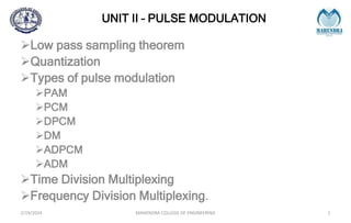
UNIT II – PULSE MODULATION
Low pass sampling theorem
Quantization
Types of pulse modulation
PAM
PCM
DPCM
DM
ADPCM
ADM
Time Division Multiplexing
Frequency Division Multiplexing.
2/19/2024 MAHENDRA COLLEGE OF ENGINEERING 1

PULSE MODULATION
 In Analog modulation both carrier and modulating signal
are in analog.
 In pulse modulation ,modulation signal is analog signal but
carrier signal is discrete pulse signal.

SAMPLING THEOREM
 This provides a mechanism for representing a continuous
time signal by a discrete time signal, taking sufficient
number of samples of signal so that original signal is
represented in its samples completely. It can be stated as:
(i) A band-limited signal of finite energy with
no frequency component higher than fm Hz, is completely
described by its sample values which are at uniform
intervals less than or equal to 1/2fm seconds apart.
[Ts=1 / 𝟐𝒇𝒎 ]where Ts is sampling time.
 Sampling frequency must be equal to or higher than 2fm
Hz. [fs ≥ 2fm]
 A continuous time signal may be completely represented
in samples and recovered back, if fs≥2fm, where fs is

SAMPLING THEOREM

ALIASING EFFECT
The overlapped region in case of under sampling represents
Aliasing effect. It can be termed as “the phenomenon of a
high-frequency component in the spectrum of a signal, taking
on the identity of a lower-frequency component in the
spectrum of its sampled version.
This effect can be removed by considering
(i) fs >2fm or
(ii) by using anti aliasing filters which are low pass filters and
eliminate high frequency components

TYPES OF SAMPLING TECHNIQUES
There are three types of Sampling Techniques
 Impulse sampling (or) Ideal Sampling (or) Instantaneous
Sampling
 Natural sampling
 Flat Top sampling (or) Rectangular Pulse Sampling
IMPULSE SAMPLING:
• Impulse Sampling is obtained by multiplying input signal x(t)
with impulse train of period 'Ts. Also called ideal
sampling. Practically not used because pulse width cannot be
zero and the generation of impulse train not possible.

NATURAL SAMPLING
 This type of sampling similar to
ideal sampling except for the fact that
instead of delta function, now we use
rectangular train of period Ts. i.e. multiply
input signal x(t) to pulse train
 An electronic switch is used to
periodically shift between the two contacts
at a rate of fs = (1/Ts ) Hz, staying on the
input contact for C seconds and on the
grounded contact for the remainder of each
sampling
 The output xs(t) of the sampler
consists of segments of x(t) and hence Xs(t)
can be considered as the product of x(t) and

Flat Top sampling:
During transmission, noise is introduced at
top of the transmission pulse which can be
easily removed if the pulse is in the form
of flat top.
Here, the top of the samples are flat i.e.
they have constant amplitude and is equal
to the instantaneous value of the baseband
signal x(t) at the start of sampling. Hence, it
is called as flat top sampling or practical
sampling.
Flat top sampling makes use of sample
and hold circuit
Theoretically, the sampled signal can be
obtained by convolution of rectangular
pulse h(t) with ideally sampled signal
,sδ(t)

APERTURE EFFECT
Spectrum of flat topped sample is given by
G(f)=fs ∑〖𝑿(𝒇−𝒏𝒇𝒔)𝑯(𝒇)〗 , where H(f)= τ.sin c(fs.t)𝒆^(−𝒋𝝅𝒇𝝉)
This equation shows that signal g(t) is obtained by passing the
signal s(t) through a filter having transfer function H(f).
Figure(a) shows one pulse of rectangular pulse train and each sample of
x(t) i.e. s(t) is convolved with this pulse
Figure (b) shows the spectrum of this pulse. Thus, flat top sampling
introduces an amplitude distortion in reconstructed signal x(t) from g(t).
There is a high frequency roll off making H(f) act like a LPF, thus
attenuating the upper portion of message signal spectrum. This is
known as aperture effect

TYPES OF PULSE MODULATION

NYQUIST RATE AND NYQUIST INTERVAL
NYQUIST RATE
When the sampling rate becomes exactly equal to 2fm
samples/ sec, for a signal bandwidth fm, then it is called Nyquist
Rate.
fs = 2fm Samples/sec
NYQUIST INTERVAL
It is the time interval between any two adjacent samples
when sampling rate is Nyquist rate.
Ts= ½ fm, Ts-> Sampling time.
QUANTIZATION
The digitization of analog signals involves the
rounding off of the values which are approximately equal to the
analog values. The method of sampling chooses a few points
on the analog signal and then these points are joined to round
off the value to a near stabilized value. Such a process is called

QUANTIZATION OF ANALOG SIGNAL
The analog-to-digital converters
perform this type of function to
create a series of digital values out
of the given analog signal. The
figure represents an analog signal.
This signal to get converted into
digital, has to undergo sampling and
quantizing.
The quantizing of an analog
signal is done by discretizing the
signal with a number of quantization
levels. Quantization is representing
the sampled values of the amplitude
by a finite set of levels, which
means converting a continuous-
amplitude sample into a discrete-

QUANTIZATION OF ANALOG SIGNAL
TYPES OF QUANTIZATION
• There are two types of
Quantization - Uniform
Quantization and Non-uniform
Quantization.
• The type of quantization in which
the quantization levels are
uniformly spaced is termed as
a Uniform Quantization. The
type of quantization in which the
quantization levels are unequal
and mostly the relation between
them is logarithmic, is termed as

PULSE AMPLITUDE MODULATION
DEFINITION
Pulse Amplitude Modulation (PAM) is an analog
modulating scheme in which the amplitude of the
pulse carrier varies proportional to the instantaneous
amplitude of the message signal.
GENERATION OF PAM

GENERATION OF PAM
Here the modulating signal is given to the low pass filter in order to
band limit the message signal.
The LPF at the beginning is placed in order to avoid aliasing of the
samples. The LPF passes only the low-frequency component of the
signal and eliminates the high-frequency signal component. The output
of LPF is then provided to a modulator, where it gets mixed with the
rectangular pulse train.
Basically, the pulsed carrier gets modulated by the message signal
here. The rectangular carrier pulse is generated by the pulse generator
circuit.
The modulator generates a pulse amplitude modulated signal. The
sampled pulses can be achieved either by natural or flat top sampling.
The output of the modulator is provided to the pulse reshaping circuit.
This basically shapes the pulses so that it can be easily detected at the

DETECTION OF NATURAL PAM
PAM signal can be detected by passing it through a
LPF which is tuned to fm.
So all high frequency ripples are removed and the
original modulating signal is recovered back

FLAT TOP PAM
• A sample of hold circuit is used to
produce flat top sampled PAM. This
consists of two FET switches and a
capacitor.
• Flat top PAM signals are generated
by applying the input modulating
signal changing switch. Sampling
switch is closed for a short duration
by a short pulse applied to gate G1
of the transistor.
• During this period, the capacitor C
quickly charged up to a voltage
equal to the instantaneous sample
value of the incoming signal.
• Now, sampling switch is opened
and capacitor C holds the charge.
The discharge switch is then closed
by a pulse applied to gate G2, Due

ADVANTAGES OF PAM
 Simple generation
 Simple detection
DISADVANTAGES OF PAM
 In PAM noise cannot be e removed easily.
 Transmission bandwidth required is too large.
 Transmission power is not constant.

PULSE CODE MODULATION PCM
Definition
Pulse code modulation is essentially an analog
to digital conversion process , where the information
contained in the instantaneous sample of analog signal
are represented by digital codes and are transmitted as a
serial bit stream.
The PCM system includes the following basic elements
• Transmitter
• Transmission path
• Receiver

PCM TRANSMITTER
The basic operations performed in the transmitter of
a PCM system are
 Sampling
 quantizing
 encoding
The quantizing and encoding operations
are usually performed in the same circuit which is
called analogue to digital converter.

LPF: The LPF are used to aliasing of the message signal by
adjusting the frequenciesgreater than fm so that a proper
sampling rate can be obtained at PCM transmitter.
Sampler:
A train of narrow rectangular pulse are used to sample the
message signal fs ≥ 2fm
Quantizer
The process of making the signal discrete in amplitude
by approximating the sampled signal to the nearest predefined or
representation level is called quantization.
It has two types
Uniform quantization, Non uniform quantization
Encoder

PCM transmission path
 The PCM transmission path is referred as the path
between PCM transmitter and PCM receiver over which
the PCM signal travel.
 The ability of controlling the effects caused by
distortion and noise in the transmission of PCM wave is
the important feature of PCM system
 PCM achieves the capacity with the help of a chain of
regenerative repeaters

PCM RECEIVER
 The noise removed pulses are applied to decoder.
 A sample and hold circuit in the decoder can be used to
convert the digitized word into to its analog value.
 Message signal is recovered by passing the decoder
output through a LPF whose cutoff frequency is equal to
the message bandwidth fm bandwidth of PCM= 1/2 Nfs,
N=No of samples

PULSE TIME MODULATION
• Pulse Time Modulation (PTM) is a class of
analog signaling technique that encodes
the sample values of an analog signal onto
the time axis of a digital signal.
• The two main types of pulse
time modulation are:
1.Pulse Width Modulation (PWM)
2.Pulse Position Modulation (PPM)

PULSE WIDTH MODULATION (PWM)
 The pulse width modulation is the modulation of signals by
varying the width of pulses. The amplitude and positions of
the pulses are constant in this modulation
 It is also known as Pulse duration modulation (PDM).
 It is a type of Pulse Time Modulation (PTM)
technique where the timing of the carrier pulse is varied
according to the modulating signal.
 Due to constant amplitude property, it gets less affected by
noise. However, during transmission channel noise
introduces some variation in amplitude as it is additive in
nature. But that is totally easy removable at the receiver by
making use of limiter circuit.
 Since the width of the pulses contains information, the
noise factor does not cause much signal distortion. Hence

GENERATION OF PWM

GENERATION OF PWM
• The message signal and the carrier waveform is fed to a
modulator which generates PAM signal. This pulse
amplitude modulated signal is fed to the non-inverting
terminal of the comparator.
• A ramp signal generated by the sawtooth generator is fed
to the inverting terminal of the comparator.
• These two signals are added and compared with the
reference voltage of the comparator circuit. The level of the
comparator is so adjusted to have the intersection of the
reference with the slope of the waveform.
• The PWM pulse begins with the leading edge of the ramp
signal and the width of the pulse is determined by the
comparator circuit.
• The width of the PWM signal is proportional to the omitted

GENERATION OF PWM
• There are three types of PWM.
– The leading edge of the pulse
being constant, the trailing edge
varies according to the message
signal. The waveform for this type
of PWM is denoted as (a) in the
above figure.
– The trailing edge of the pulse
being constant, the leading edge
varies according to the message
signal. The waveform for this type
of PWM is denoted as (b) in the
above figure.
– The center of the pulse being
constant, the leading edge and
the trailing edge varies
according to the message signal.

WAVEFORM OF GENERATION OF PWM

DETECTION OF PWM

DETECTION OF PWM
• As we know during signal transmission, some noise gets
added to the PWM signal. So firstly to remove the noise
introduced in the transmitted signal, the incoming signal is fed
to a pulse generator. This regenerates the PWM signal.
• This regenerated PWM pulse is then given to a reference
pulse generator that generates pulses of constant amplitude
along with constant width.
• The regenerated pulses are also given to the ramp signal
generator, that generates a ramp signal of constant slope,
whose duration is similar to the pulse duration. Thus we have
ramp signal height proportional to the PWM pulse width.
• The constant amplitude pulses are then provided to a
summation unit in order to get added with the ramp signal.
The added output is then fed to a clipper, this clips off the
signal up to its threshold value thereby generating a PAM

WAVEFORM OF DETECTION OF PWM

ADVANATAGES AND DISADVANTAGES OF PWM
ADVANTAGES OF PWM
 Less effect of noise , very good noise immunity
 Synchronisation between the transmitter and receiver is not
essential
 It is possible to reconstruct the PWM signal signal from a
noise or contaminated PWM.
DISADVANTAGES OF PWM
 Due to changing width of the pulses, variation in
transmission power is also noticed.
 Bandwidth requirement in case of PWM is somewhat larger
than PAM.
APPLICATIONS OF PULSE WIDTH MODULATION
 It is used in telecommunications, brightness controlling of
light or speed controlling of fans etc.

PULSE POSITION MODULATION (PPM)
DEFINITION:
A modulation technique that allows variation in
the position of the pulses according to the amplitude of
the sampled modulating signal is known as Pulse Position
Modulation (PPM). It is another type of PTM, where the
amplitude and width of the pulses are kept constant and
only the position of the pulses is varied
• The information is transmitted with the varying position
of the pulses in pulse position modulation.
• The pulse displacement is directly proportional to the
sampled value of the message signal.

GENERATION OF PPM

GENERATION OF PPM
• A PAM signal is produced with is further processed at
the comparator in order to generate a PWM signal.
• The output of the comparator is fed to a monostable
multivibrator. It is negative edge triggered. Hence, with
the trailing edge of the PWM signal, the output of the
monostable goes high.
• This is why a pulse of PPM signal begins with the
trailing edge of the PWM signal.
• It is to be noted in case of PPM that the duration for
which the output will be high depends on the RC
components of the multivibrator. This is the reason
why a constant width pulse is obtained in case of the
PPM signal.
• With the modulating signal, the trailing edge of PWM
signal shifts, thus with that shift, the PPM pulses

GENERATION OF PPM
• Pulse Position Modulation (PPM) is an analog
modulation scheme in which, the amplitude and the
width of the pulses are kept constant, while the
position of each pulse, with reference to the
position of a reference pulse varies according to the
instantaneous sampled value of the message signal.
• The transmitter has to send synchronizing pulses (or
simply sync pulses) to keep the transmitter and the
receiver in sync. These sync pulses help to maintain
the position of the pulses. The following figures
explain the Pulse Position Modulation.
• Pulse position modulation is done in accordance with
the pulse width modulated signal. Each trailing edge
of the pulse width modulated signal becomes the
starting point for pulses in PPM signal. Hence, the
position of these pulses is proportional to the width
of the PWM pulses

WAVEFORM OF PPM

DETECTION OF PPM

DETECTION OF PPM
• The PPM signal transmitted from the modulation circuit
gets distorted by the noise during transmission. This
distorted PPM signal reaches the demodulator circuit.
The pulse generator employed in the circuit generates a
pulsed waveform. This waveform is of fixed duration
which is fed to the reset pin (R) of the SR flip-flop.
• The reference pulse generator generates, reference
pulse of a fixed period when transmitted PPM signal is
applied to it. This reference pulse is used to set the flip-
flop.
• These set and reset signals generate a PWM signal at
the output of the flip-flop. This PWM signal is then further
processed in order to provide the original message

ADVANATAGES AND DISADVANTAGES OF PPM
ADVANTAGES OF PWM
• Similar to PWM, PPM also shows better noise immunity as
compared to PAM. This is so because information content is
present in the position of the pulses rather than amplitude.
• As the amplitude and width of the pulses remain constant. Thus
the transmission power also remains constant and does not
show variation.
• Recovering a PPM signal from distorted PPM is quite easy.
• Interference due to noise in more minimal than PAM and PWM.
DISADVANTAGES OF PULSE POSITION MODULATION
• In order to have proper detection of the signal at the receiver,
transmitter and receiver must be in synchronization.
• The bandwidth requirement is large.
APPLICATIONS OF PULSE POSITION MODULATION
• The technique is used in an optical communication system, in
radio control and in military applications.

ADVANTAGES AND DISADVANTAGES OF PPM
PAM PWM PPM
Amplitude is varied Width is varied Position is varied
Bandwidth depends on the width
of the pulse
Bandwidth depends on the rise
time of the pulse
Bandwidth depends on the rise
time of the pulse
Instantaneous transmitter power
varies with the amplitude of the
pulses
varies with the amplitude and
the width of the pulses
remains constant with the width
of the pulses
System complexity is high System complexity is low System complexity is low
Noise interference is high Noise interference is low Noise interference is low

LINE CODING
2/19/2024 MAHENDRA COLLEGE OF ENGINEERING
LINE CODES:
These codes are various formats (waveforms) for
representing the binary sequence. They are called as line
codes. It is also known as data transmission codes or
modulation codes.
DEFINITION
It is the process of converting binary data, a sequence of
bits to a digital data. The data, text, numbers, graphical
images, audio and video which are stored in computer
memory are in the form of sequences of bits. Line Coding
converts these sequences into signals
53

LINE CODING
At the sender side digital data are encoded into a
digital signal and at the receiver side the digital
data are recreated by decoding the digital signal.
54

MAPPING DATA SYMBOLS ONTO SIGNAL LEVELS
• A data symbol (or element) can consist of a number of
data bits:
• 1 , 0 or
• 11, 10, 01, …
…
• A data symbolcan be codedinto a singlesignal element
or multiple signal elements
• 1 -> +V, 0 -> -V
• 1 -> +V and -V, 0 -> -V and +V
• The ratio ‘r’ is the number of data elements carried by a
55

RELATIONSHIP BETWEEN DATA RATE AND SIGNAL
RATE
• The data rate defines the number of bits sent per sec-
bps. It is often referred to the bit rate.
• The signal rate is the number of signal elements sent
in a second and is measured in bauds. It is also
referred to as the baud rate.
• Goal is to increase the data rate whilst reducing the
baud rate.
56

SIGNAL ELEMENT VERSUS DATA ELEMENT
r = number of data elements / number
of signal elements

CONSIDERATIONS ABOUT LINE CODING
• Transmission Bandwidth
The transmission bandwidth should be as small as possible.
• Power Efficiency
For a given bandwidth and specified error rate the
transmitted power should be as low as possible.
• Self synchronization
The clocks at the sender and the receiver must
have the same bit interval. If the receiver clock is faster
or slower it will misinterpret the incoming bit stream. It
may become the source of incorrigible errors.
58

Effect of lack of synchronization
59

• Error detection
• errors occur during transmission due to line impairments.
• Some codes are constructed such that when an error occurs
it can be detected.
• For example: a particular signal transition is not part of the
code. When it occurs, the receiver will know that a symbol
error has occurred.
• Noise and interference
• there are line encoding techniques that make the transmitted
signal “immune” to noise and interference.
• This means that the signal cannot be corrupted, it is stronger
than error detection.
• Complexity
• the more robust and resilient the code, the more complex it
is to implement and the price is often paid in baud rate or

• Baseline wandering:
• a receiver will evaluate the average power of the
received signal (called the baseline) and use that to
determine the value of the incoming data elements.
• If the incoming signal does not vary over a long period of
time, the baseline will drift and thus cause errors in
detection of incoming data elements.
• A good line encoding scheme will prevent long runs of
fixed amplitude.

• DC components
• When the voltage level in a digital signal is constant for a
while, the spectrum creates very low frequencies (results
of Fourier analysis).
• These frequencies around zero, call DC (direct-current)
components, present problems for a system that cannot
pass low frequencies or a system that uses electrical
coupling (via a transformer).
• For example, a telephone line cannot pass frequencies
below 200 Hz.

LINE CODING CLASSIFICATION

UNIPOLAR – NRZ & RZ
• In unipolar format, the waveform has a single
polarity.
• The waveform can have +5 or +12 volts when high.
• The waveform is simple On-Off.
UNIPOLAR RZ – Waveform and Expression
In the unipolar RZ form, the waveform has
zero value when symbol 1 is transmitted and
waveform has A volts when 1 is transmitted.
In the RZ form, the A volts is present for Tb / 2
period if symbol 1 is transmitted and for remaining
T / 2 , waveform returns value., for unipolar RZ 64

UNIPOLAR NRZ : WAVEFORM AND EXPRESSION
A unipolar NRZ (not return to zero) format, when
symbol 1 is transmitted the signal has A volts for full
duration. When symbol 0 is to be transmitted, the signal
has zero volts (no signal) for completed symbol duration
66

POLAR – NRZ & RZ
POLAR RZ: Waveform and expression
67

POLAR – NRZ & RZ
POLAR NRZ: Waveform and expression
68

BIPOLAR NRZ (ALTERNATE MARK INVERSION)
BIPOLAR NRZ:
In this format, the successive 1s are represented
by pulses with alternate polarity and zeros are
represented by no pulses
69

DPCM – DIFFERENTIAL PULSE CODE MODULATION
• In PCM, each sample of the
waveform is encoded
independently of all the other
samples.
• The average change in
amplitude between
successive samples is
relatively small.
• Hence an encoding scheme
that exploits the redundancy
in the samples will result in a
lower bit rate for the source
output.

DPCM – DIFFERENTIAL PULSE CODE
MODULATION
• In DPCM we encode the differences between
successive samples rather than the samples.
• Since differences between samples are expected to
be smaller than the actual sampled amplitudes, fewer
bits are required to represent the differences.
• In this case we quantize and transmit the differenced
signal sequence
• The differential pulse code modulation works on the
principle of prediction. The value of the present
sample is predicted from the past samples.
• The prediction may not be exact but it is very close to
the actual sample value.
71

• Need of Predictor:
• When the sampling rate is set at the nyquist rate, it generates
unacceptably excessive quantization noise in comparison to
PCM.(in some cases signal may change drastically, change may
be +ve or -ve)
• If we increase the sampling rate the quantization noise may
decrease but the bit rate of DPCM (bits per sample x sample
rate) may exceeds the bit rate of PCM.
• It is improved by recognizing that there is a co- relation between
successive samples of the signals.
• A natural refinement of this general approach is to predict the
current sample based on the previous M samples utilizing linear
prediction (LP), where LP parameters are dynamically estimated.
• Hence predictor is something which can predict the range of next
required increment to the past value in order to produce the
present value with some probability of being correct.
73

ADAPTIVE DIFFERENTIAL PULSE CODE
MODULATION- ADPCM

MODULATION- ADPCM
 ADPCM is a technique for converting sound or analog
information to binary information(a sting of 0s and 1s) by
taking frequent samples of the sound and expressing the
value of the sampled sound modulation in binary terms
 ADPCM is a variant of DPCM that varies the size of the
quantization step, to allow further reduction of the required
data bandwidth for a given signal to noise ratio
 Typically, the adaption to signal statistics in ADPCM consists
simply of an adaptive scale factor before quantizing the
difference in the DPCM encoder
 Adaptive DPCM further improves the efficiency of DPCM
encoding by incorporating an adaptive quantizer at the 80

MODULATION- ADPCM
DESIGN OBJECTIVES
 Remove redundancies from speech signals
 Assign available bits to encode non-redundant parts of
speech signal in an efficient way
 Standard PCM is at 64 kb/s – can be reduced to 32, 16, 8 or
even 4 kb/s
 Price = proportionally increased complexity
 For same speech quality but Half the bit rate - Computational
complexity is an order of magnitude higher 81

MODULATION- ADPCM
ADPCM PRINCIPLES
82
• Allows encoding of speech at 32 kb/s – requires 4 bits
per sample
• Uses adaptive quantization and adaptive prediction
– adaptive quantization – uses a time-varying step Δ[n].
The step-size is varied to match the input signal σM
2
• φ is a constant; σ– estimate of the standard deviation -
has to be computed continuously
ˆ
[ ] [ ]
M
n n

 
ˆ

ˆ

ˆ


MODULATION- ADPCM
– adaptive quantization with forward
estimation (AQF) – uses
unquantized samples of the input
signal to derive forward estimates
of σM[n]; requires a buffer to store
samples for a certain learning
period; incurs delay (~ 16 ms for
speech)
– adaptive quantization with
backward estimation (AQB) –
uses samples of the quantizer
output to derive backwards
estimates of σ [n]

DELTA MODULATION

DELTA MODULATION
WORKING OF TRANSMITTER
• The summer in the accumulator adds quantizer output(+ or -
Δ) with the previous sample approximation. This gives the
present sample approximation,
u(nTs) = u (nTs - Ts) + [ +/- Δ]
u(nTs) = u [(n-1)Ts)] + b(nTs)
• The previous sample approximation u[(n-1)Ts] is restored by
delaying one sample period Ts.
• The Sampled input signal x(nTs) and staircase approximated
signal x^(nTs) are subtracted to get error signal e(nTs)
• Thus depending on the sign of e(nTs), one bit quantizer
generates an output of +Δ or –Δ. If the step size is +Δ, then a
binary 1 is transmitted and if the step size is –Δ, then a binary

DELTA MODULATION
WORKING OF RECEIVER
• The DM receiver uses a accumulator and a low pass filter.
The accumulator generates the staircase approximated signal
output and is delayed by one sampling period Ts.
• It is then added to the input signal. If input is binary 1 then it
adds + Δ step to the previous output which is delayed.
• If the input is binary 0 then one step Δ is subtracted from the
delayed signal.
• Also the low pass filter cuts off high frequency in x(t). This low

ADVANTAGES OF DELTA MODULATION
ADVANTAGES
Delta Modulation has certain advantages over Pulse code
Modulation:
(i) Since Delta modulation transmits only one bit for one
sample, therefore the signalling rate and transmission
channel bandwidth is quite small for delta modulation
compared to PCM
(ii) The transmitter and receiver implementation is very much
simple for delta modulation.
(iii) There is no requirement of analog to digital converters in
delta modulation
DRAWBACKS OF DELTA MODULATION

SLOPE OVERLOAD
DISTORTION
 This distortion arises
because of large dynamic
range of the input signal
 As the fig shows, the rate of
rise of input signal is very high
that the staircase signal
cannot approximate it, the
step size Δ becomes too small
for staircase signal u(t) to
follow the step segment of x(t)
 Hence there is a large error
between the staircase

GRANULAR or IDEAL NOISE
 Granular or ideal noise
occurs when the step size is too
large compared to small
variations in the input signal.
 For very small variation in the
input signal, the staircase signal
is changed by large amount Δ
because of large step size.
 When the input signal is almost
flat the staircase signal u(t)
keeps on oscillating by +/- Δ
around the signal

ADAPTIVE DELTA MODULATION

• The entire operation of receiver is divided into two parts. In
the first stage, for each incoming bit the step size is
produced.
• The step size is decided by both previous and present input
• Then it is applied to the accumulator whose function is to
generate staircase
waveform depending on the input applied to it
• Finally the original message signal is reconstructed from the

COMPARISON OF PCM, DPCM, DM, ADM
PARAMETER PCM DM ADM DPCM
No of bits or
Sample N can be
4,8,16,32…
N=1 N=1 N is more than
1
Step size Depends on Q-
level
Step size is
fixed
Step size is
variable
Step size is
fixed.
Errors Quantization
errors
Slope overload
& Granular
Errors.
Granular Errors Slope Overload
& Granular
Signal rate High Low Low Lower than
PCM
System
Complexity
Complex Simple Simple Simple
Noise
Immunity Very Good Very Good Very Good Very Good

CHANNEL VOCODERS

CHANNEL VOCODER

MULTIPLEXING
• Multiplexing is the set of techniques that allows the
simultaneous transmission of multiple signals across a
single data link.
• A Multiplexer (MUX) is a device that combines
several signals into a single signal.
• A Demultiplexer (DEMUX) is a device that performs
the inverse operation

MULTIPLEXING

FREQUENCY-DIVISION MULTIPLEXING
(FDM)
FDM is an analog technique that can be applied when
the bandwidth of a link is greater than the combined
bandwidths of the signals to be transmitted.
In FDM signals generated by each device modulate
different carrier frequencies. These modulated signals
are combined into a single composite signal that can be
transported by the link.

(FDM)
• In FDM signals generated by each device modulate
different carrier frequencies. These modulated signals
are combined into a single composite signal that can
be transported by the link.
• Carrier frequencies are separated by enough
bandwidth to accommodate the modulated signal.
• These bandwidth ranges arte the channels through
which various signals travel.
• Channels must separated by strips of unused
bandwidth (guard bands) to prevent signal
overlapping.

(FDM)
FDM TRANSMITTER SECTION
• The numerous signals that are to be transmitted along a
common channel modulate different carriers in the
modulating section. The output of the modulator will
have multiple signals of different carrier frequency.
• The modulated signals are then fed to a linear mixer
which is different from a normal mixer.
• Linear mixer simply produces the algebraic sum of the
generated modulated signals. The combined signal at
the output of the mixer is then transmitted along a
single channel.

(FDM)
FDM RECEIVER SECTION
• The receiver section will have a composite signal that was
transmitted by the linear mixer over a channel.This
composite signal is then fed to different filters mainly BPF
each having a centre frequency corresponding to the carrier
frequency.
• The BPF passes the channel information without any
distortion. BPF rejects signals of all other frequencies and
accepts the signal of the desired centre frequency.
• Further, the signals after being processed by the BPF goes
to individual demodulator section where demodulation of
the signals takes place to separate modulating signal from
that of the carrier signal.

(FDM)

TIME DIVISION MULTIPLEXING (TDM)
Digital Multiplexing
The term digital represents the discrete bits of
information. Hence, the available data is in the form of
frames or packets, which are discrete.
Time Division Multiplexing (TDM)
In TDM, the time frame is divided into slots. This
technique is used to transmit a signal over a single
communication channel, by allotting one slot for each
message.
Of all the types of TDM, the main ones are
Synchronous and Asynchronous TDM.

TIME-DIVISION MULTIPLEXING

• The technique efficiently utilizes the complete channel for data
transmission hence sometimes known as PAM/TDM. This is
so because a TDM system uses a pulse amplitude
modulation. In this modulation technique, each pulse holds
some short time duration allowing maximal channel usage.
• Here at the beginning, the system consists of multiple LPF
depending on the number of data inputs. These low pass
filters are basically anti-aliasing filters that eliminate the
aliasing of the data input signal.
• The output of the LPF is then fed to the commutator. As per
the rotation of the commutator the samples of the data inputs
are collected by it. Here, fs is the rate of rotation of the
commutator, thus denotes the sampling frequency of the

• Suppose we have n data inputs, then one after the other,
according to the rotation, these data inputs after getting
multiplexed transmitted over the common channel.
• Now, at the receiver end, a de-commutator is placed that is
synchronized with the commutator at the transmitting end. This de-
commutator separates the time division multiplexed signal at the
receiving end.
• The commutator and de-commutator must have same rotational
speed so as to have accurate demultiplexing of the signal at the

SYNCHRONOUS TIME-DIVISION MULTIPLEXING
• In synchronous time-division multiplexing, the term
synchronous means that the multiplexer allocates
exactly the same time slot to each device at all times,
whether or not a device has anything to transmit.
Frames
Time slots are grouped into frames. A frame
consists of a one complete cycle of time slots,
including one or more slots dedicated to each sending
device.

• Synchronous TDM: In this technique, the time slots
are assigned at the beginning, irrespective of the idea
about the presence of data at the source. This leads to
the wastage of the channel capacity. As in the
absence of any data unit, that particular time slot gets
entirely wasted.

ASYNCHRONOUS TIME-DIVISION
MULTIPLEXING
• Asynchronous TDM: It is also termed as statistical or
intelligent TDM technique as it eliminates the drawback of
wastage of time slot present in synchronous TDM.
• Here, a particular frame is transmitted by the transmitting end
only when it gets completely filled by the data units. It exhibits
higher efficiency than that of synchronous TDM technique as it
requires smaller transmission time and ensures better
bandwidth utilization.

Communication engineering notes uniit ii

Recommended

Recommended

More Related Content

Similar to Communication engineering notes uniit ii

Similar to Communication engineering notes uniit ii (20)

Recently uploaded

Recently uploaded (20)

Communication engineering notes uniit ii