1. The document discusses the chain rule for functions of several variables. It provides examples of how to use a "tree diagram" to represent variable dependencies and derive the appropriate chain rule statement.
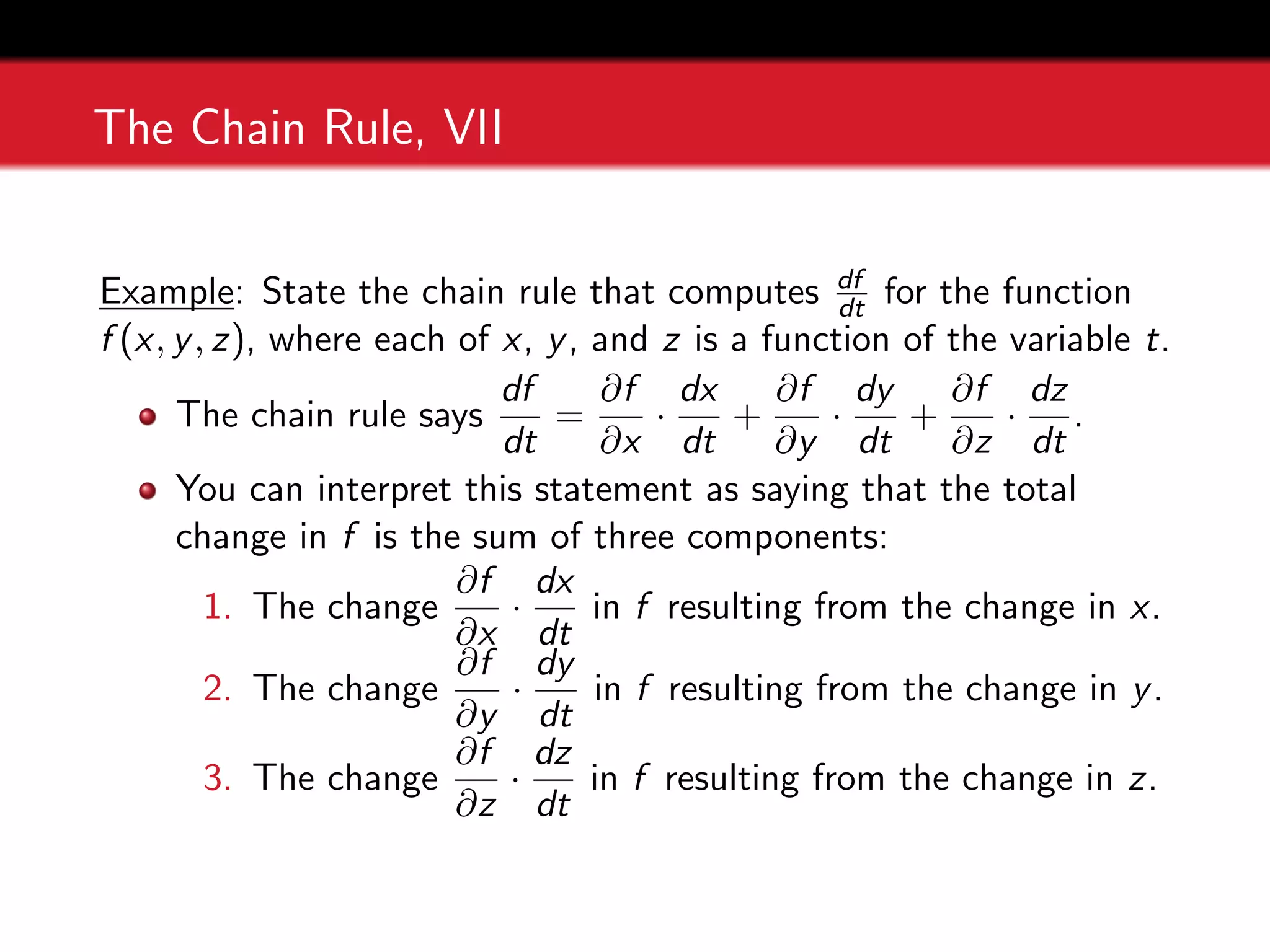
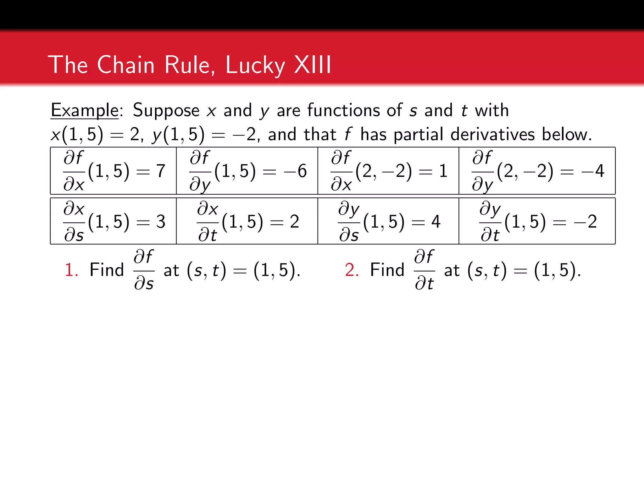
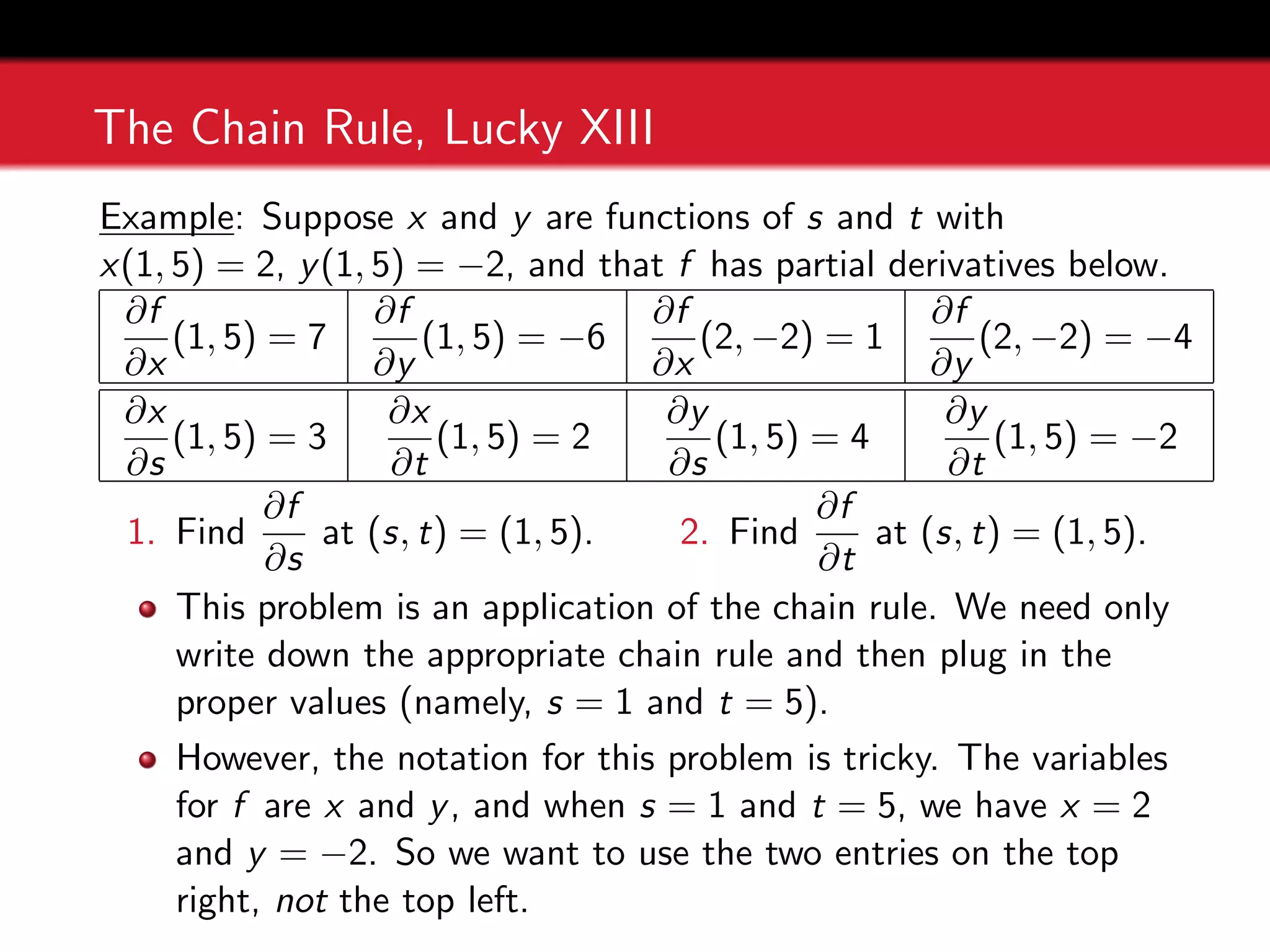
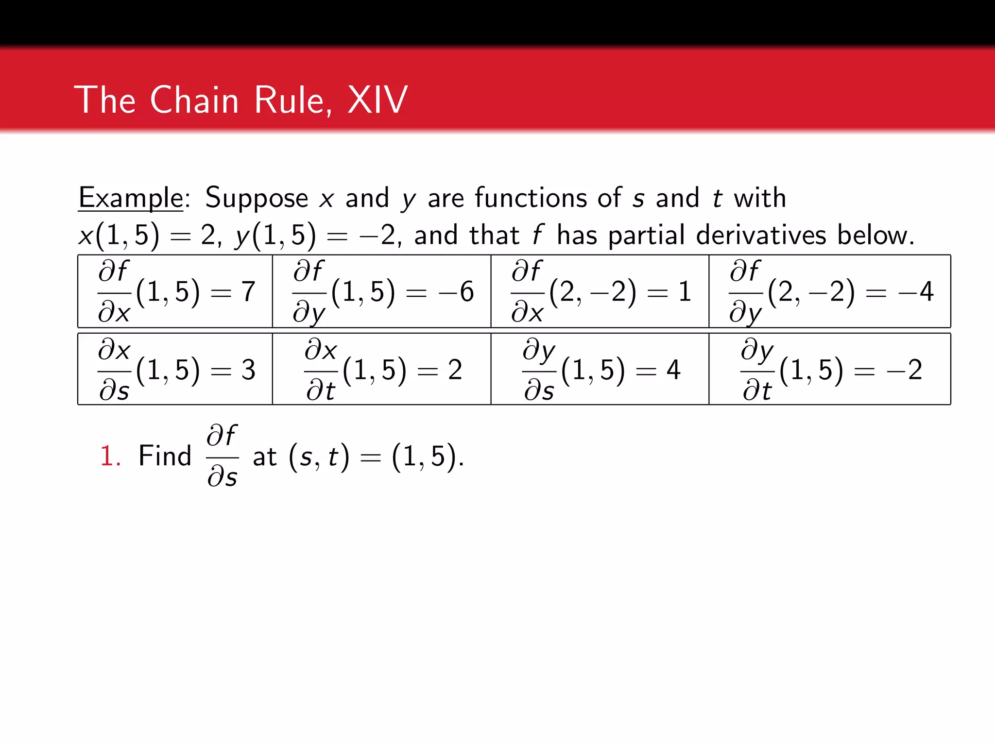
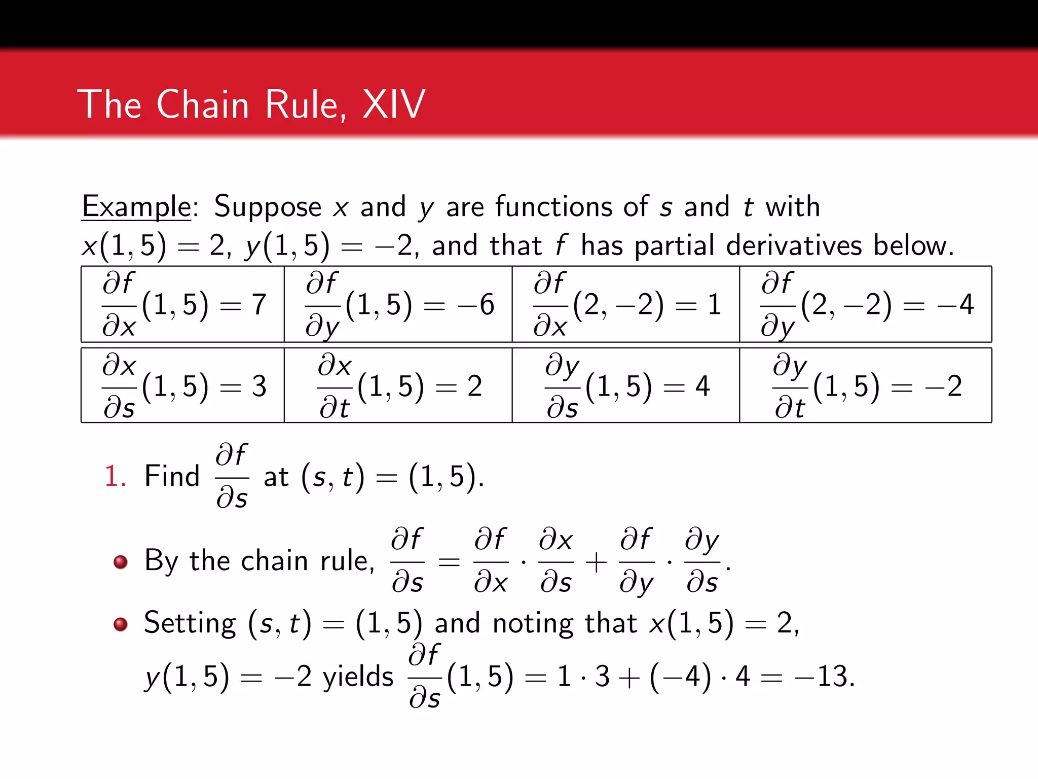
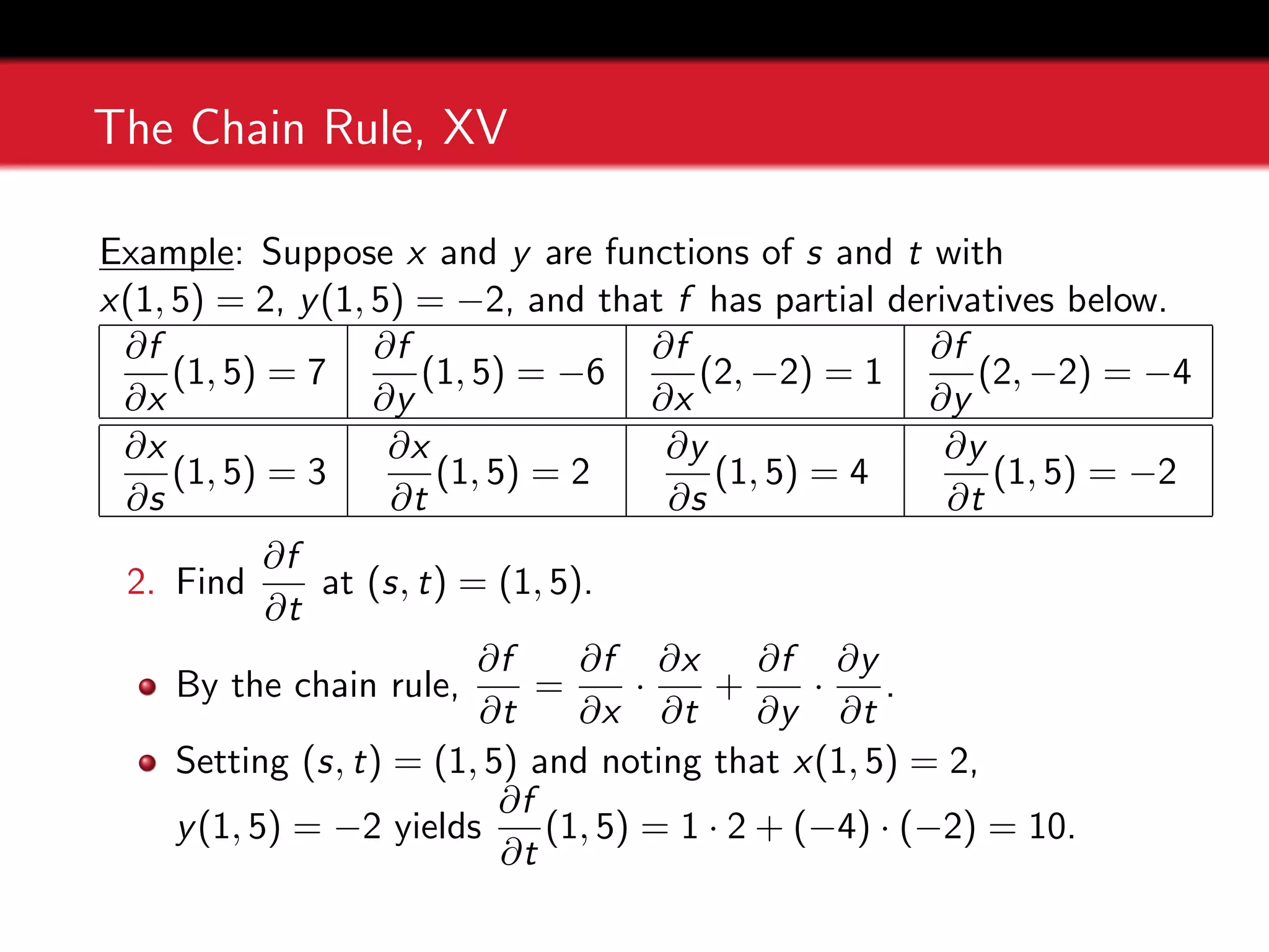
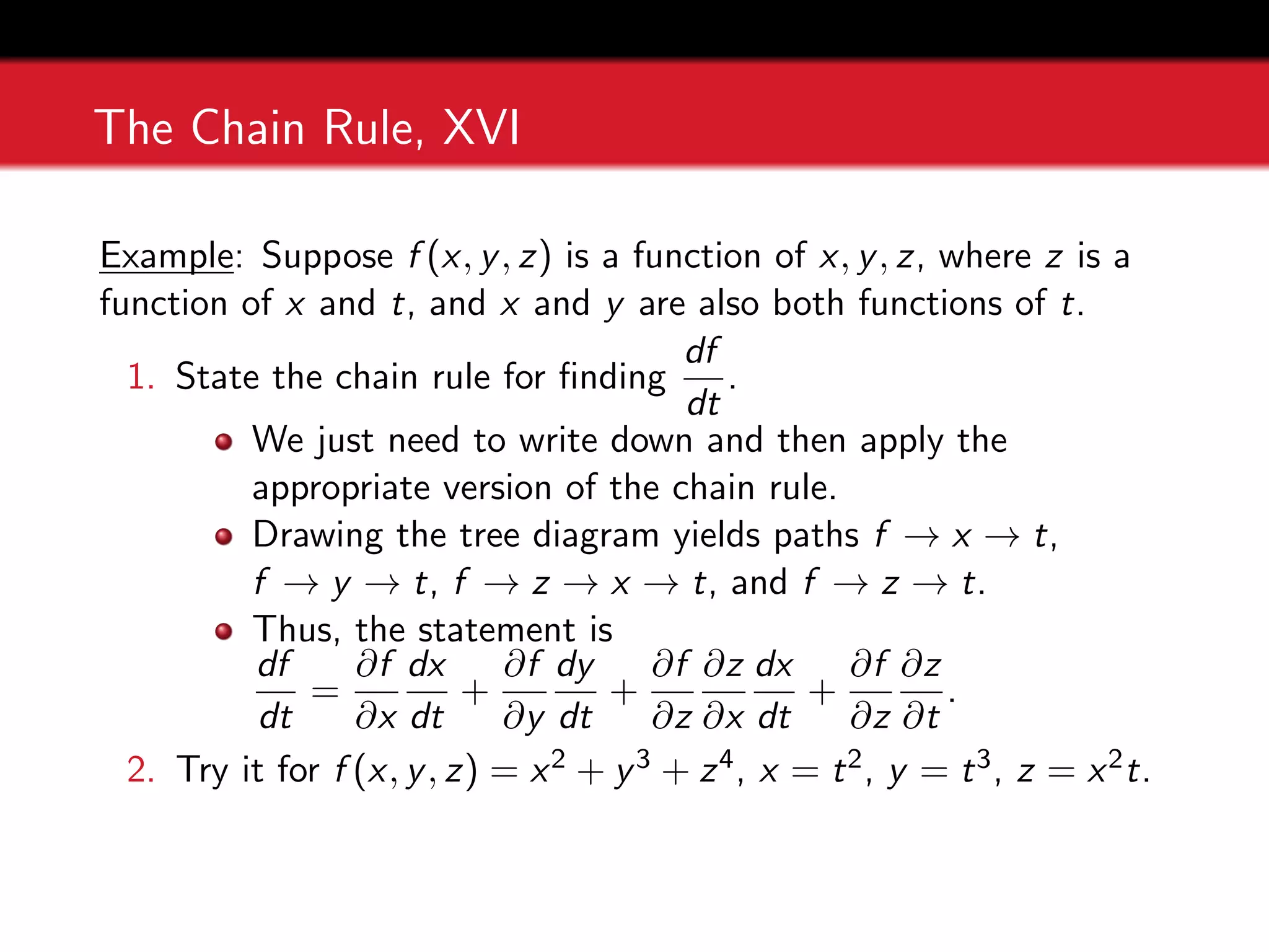
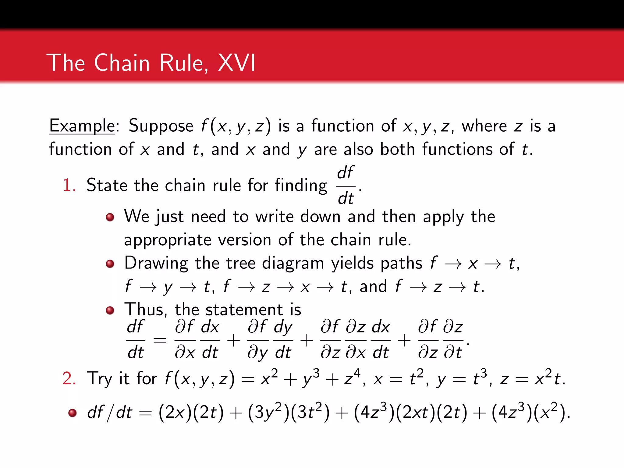
2. It also gives examples of applying the chain rule to find derivatives like df/dt for functions where variables like x, y, and z depend on t, or to find partial derivatives like ∂f/∂s and ∂f/∂t.
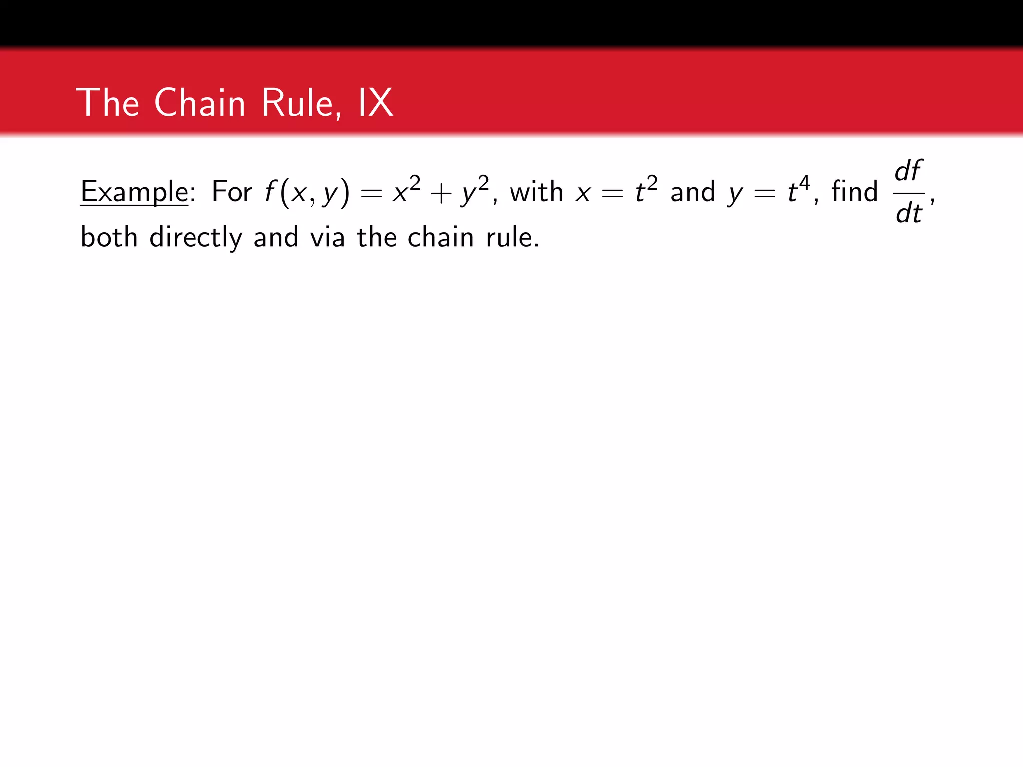
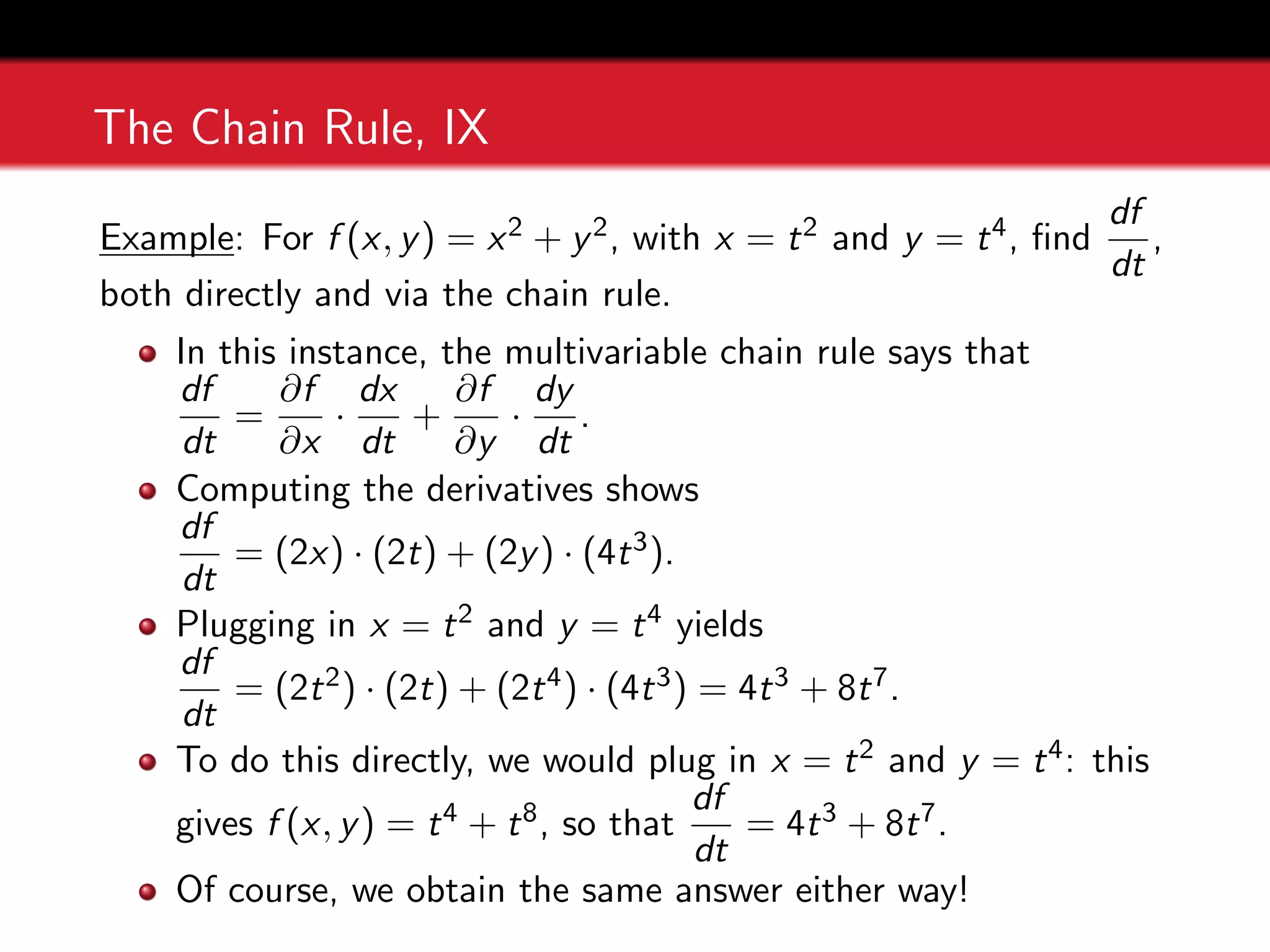
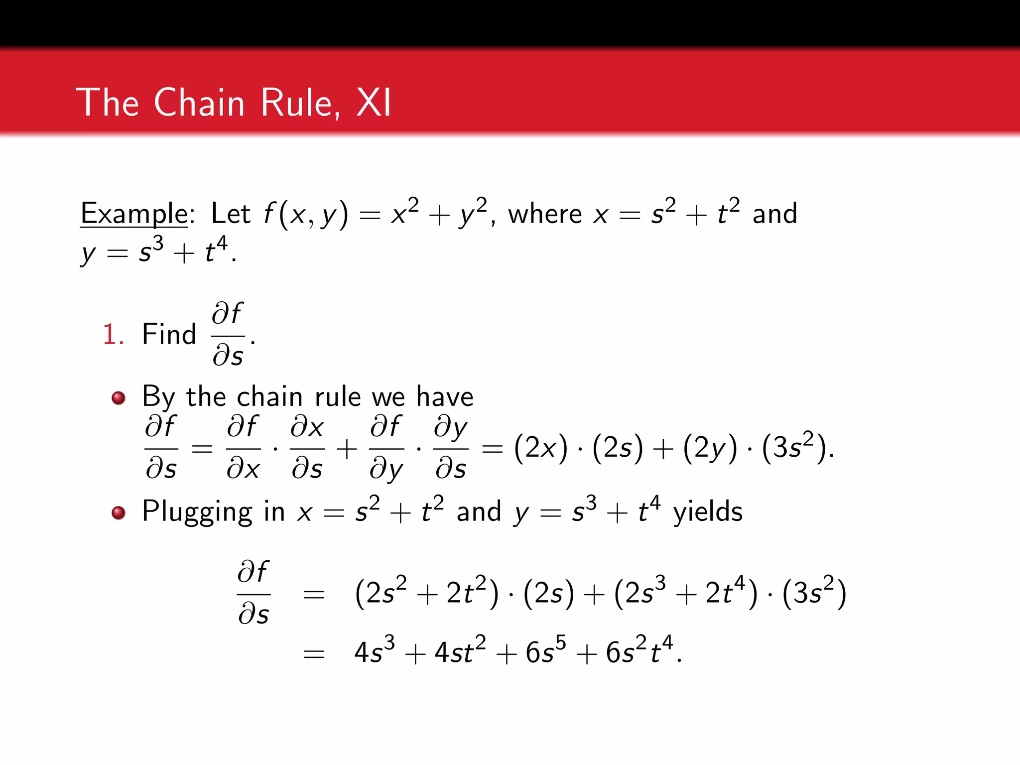
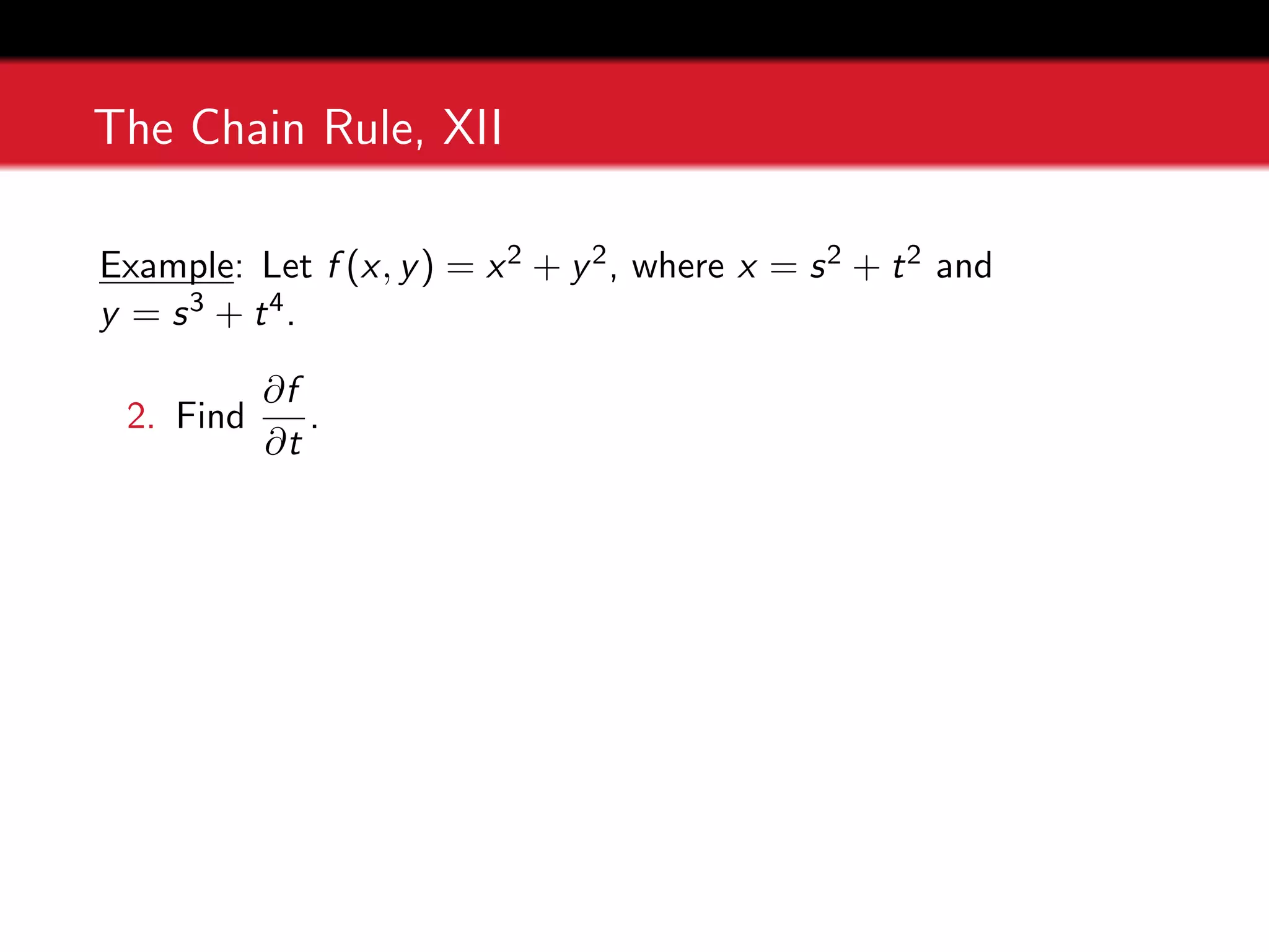
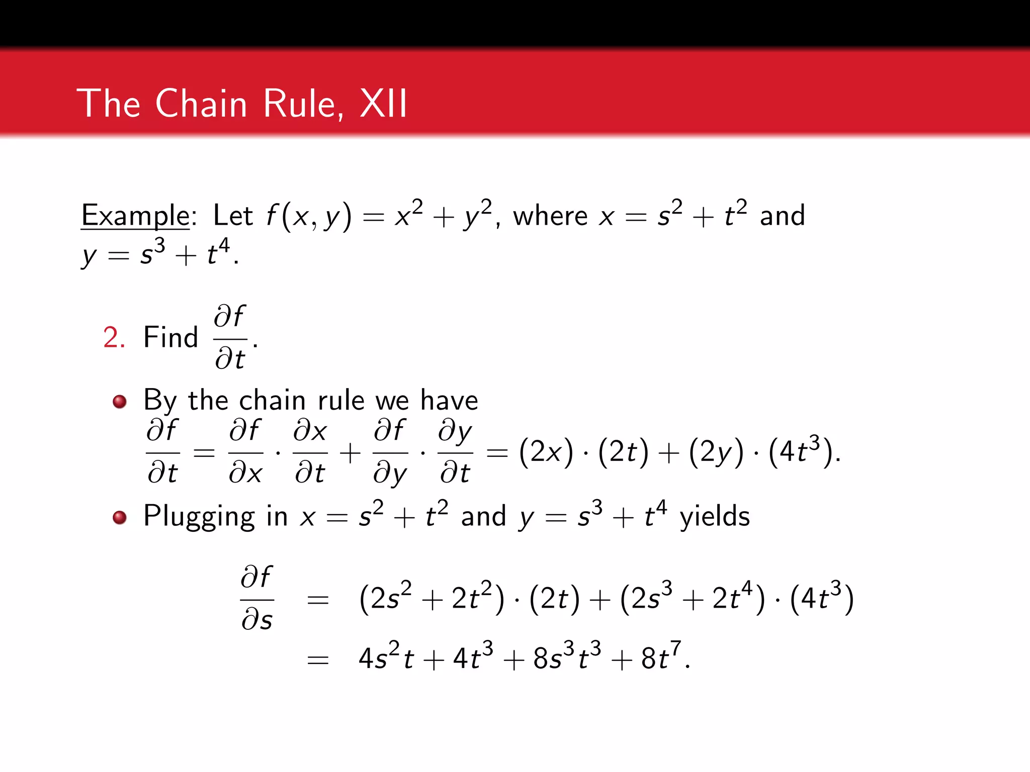
3. One example works through applying the chain rule to find df/dt for the function f(x,y) = x^2 + y^2, where x = t^2 and y = t^4, and verifies the
This document discusses the chain rule for functions of multiple variables. It begins by reviewing the chain rule for single-variable functions, then extends it to functions of more variables. The chain rule is presented for cases where the dependent variable z is a function of intermediate variables x and y, which are themselves functions of independent variables s and t. General formulas are given using partial derivatives. Examples are worked out, such as finding the derivative of a function defined implicitly by an equation. Diagrams are used to illustrate the relationships between variables.
This document summarizes a lecture on multivariable calculus that introduces limits and partial derivatives. It begins with an overview of limits in multiple variables and how they generalize limits from single variable calculus. It then defines partial derivatives, which measure how a function changes with respect to one variable while holding others constant. Examples are provided to demonstrate computing partial derivatives using differentiation rules.
The document discusses differentiation rules for products and quotients of functions. It begins by introducing the product rule, which states that the derivative of a product of two functions f and g is equal to f times the derivative of g plus g times the derivative of f. Next, it derives the quotient rule through a similar process, concluding that the derivative of a quotient of two functions u and v is equal to the denominator v times the derivative of the numerator u minus the numerator u times the derivative of the denominator v, all over the square of the denominator v squared. Several examples are provided to demonstrate applying these rules to find derivatives.
The document discusses concepts related to partial differentiation and its applications. It covers topics like tangent planes, linear approximations, differentials, Taylor expansions, maxima and minima problems, and the Lagrange method. Specifically, it defines the tangent plane to a surface at a point using partial derivatives, describes how to find the linear approximation of functions, and explains how to find maximum and minimum values of functions using critical points and the second derivative test.
The document presents information on partial differentiation including:
- Partial differentiation involves a function with more than one independent variable and partial derivatives.
- Notation for partial derivatives is presented.
- Methods for computing first and higher order partial derivatives are explained with examples.
- The concepts of homogeneous functions and the chain rule for partial differentiation are defined.
Website Designing Company is fastest growing company in the IT market in the world for the website design and website layout. we are best website designing company in India as well as in USA we are based in Noida and Delhi NCR. Website designing company is powered by Css Founder.com
In mathematics, a partial derivative of a function of several variables is its derivative with respect to one of those variables, with the others held constant (as opposed to the total derivative, in which all variables are allowed to vary). Partial derivatives are used in vector calculus and differential geometry.
This document provides an overview of functions of several variables. It discusses notation for functions with multiple independent variables, domains of such functions, and graphs of functions with two or more variables. Specifically, it gives examples of finding the domain of functions defined by equations, sketching the graph of a function as a surface in 3D space using traces in coordinate planes and parallel planes, and creating a contour map using level curves representing different values of the dependent variable.
This document provides an introduction to partial differentiation, including:
- Defining partial derivatives and how they are calculated by treating all but one variable as a constant
- Examples of finding partial derivatives using the product, quotient, and chain rules
- Higher order partial derivatives and mixed partial derivatives
- Notation for partial derivatives
- A quiz on partial derivatives concepts
1) The document discusses partial derivatives, which involve differentiating functions of two or more variables with respect to one variable while holding the others fixed. It provides definitions, examples of computing partial derivatives, and interpretations as rates of change.
2) Techniques covered include implicit differentiation, using the chain rule to find derivatives of implicitly defined functions, and computing second order partial derivatives.
3) Diagrams and tables are referenced to illustrate level curves and contour maps for functions of two variables.
1) The document discusses partial derivatives, which involve differentiating functions of two or more variables with respect to one variable while holding the others constant. It provides examples of computing first and second partial derivatives.
2) Implicit differentiation is introduced as a way to find partial derivatives of functions defined implicitly rather than explicitly. The chain rule is also discussed.
3) Methods are presented for finding partial derivatives of functions of two or three variables, including using implicit differentiation and the chain rule. Examples are provided to illustrate these concepts.
This document discusses continuity of complex fuzzy functions. It begins with introductions to fuzzy complex numbers and fuzzy complex analysis. It then provides definitions of fuzzy type I-continuity and II-continuity of complex fuzzy functions mapping generalized rectangular valued bounded closed complex complement normalized fuzzy numbers into itself. Several theorems are proved regarding the continuity of complex fuzzy functions, including that the sum, product, and composition of continuous complex fuzzy functions are also continuous.
The document discusses techniques for calculating derivatives of functions, including:
- Using formulas and theorems to calculate derivatives more efficiently than using the definition of a derivative.
- Applying rules like the power rule, product rule, and quotient rule to take derivatives.
- Using derivatives to find equations of tangent lines and instantaneous rates of change.
This document discusses the difference between ordinary derivatives and partial derivatives. Ordinary derivatives are taken with respect to one independent variable, while partial derivatives treat all other variables as constant except for the variable being differentiated. The document provides examples of calculating ordinary and partial derivatives for functions of two variables. It also notes that partial derivatives are used in the chain rule to compute ordinary derivatives for functions with multiple variables.
1. The document discusses the concept of derivatives and how to calculate them. It defines key terms like increment, average rate of change, and instantaneous rate of change.
2. Methods are provided for calculating the derivative of various types of functions, including polynomials, rational functions, and functions with roots. Examples are worked through step-by-step.
3. The relationship between derivatives and tangent lines is explained, with derivatives defined as the instantaneous rate of change or slope of the curve at a point.
Derivatives and it’s simple applicationsRutuja Gholap
The document provides an introduction to derivatives and their applications. It defines the derivative as the rate of change of a function near an input value and discusses how it relates geometrically to the slope of the tangent line. It then gives examples of finding the derivatives of common functions like constants, polynomials, and exponentials. The document also covers basic derivative rules like the constant multiple rule, sum and difference rules, product rule, and quotient rule. Finally, it discusses applications of derivatives in topics like physics, such as calculating velocity and acceleration from a position function.
This document discusses numerical methods for solving partial differential equations (PDEs). It begins by classifying PDEs as parabolic, elliptic, or hyperbolic based on their coefficients. It then introduces finite difference methods, which approximate PDE solutions on a grid by replacing derivatives with finite differences. In particular, it describes the forward time centered space (FTCS) scheme for solving the 1D heat equation numerically and analyzing its stability using von Neumann analysis.
This document discusses several topics related to calculus including:
1) Derivatives of position, velocity, and acceleration and how they relate to each other.
2) An example problem calculating velocity from a position function.
3) The Mean Value Theorem and how to apply it to find critical points of a function.
4) How the first and second derivatives of a function relate to critical points, maxima, minima, and points of inflection or concavity.
5) Related rates problems and how to set them up using derivatives and relationships between variables.
A partial differential equation contains one dependent variable and more than one independent variable. The partial derivatives of a function f(x,y) with respect to x and y at a point (x,y) are represented as ∂f/∂x and ∂f/∂y. Higher order partial derivatives can be found by taking partial derivatives multiple times with respect to the independent variables. The chain rule can be used to find partial derivatives when the dependent variable is a function of other variables that are themselves functions of the independent variables.
The document discusses implicit differentiation. It explains that implicit differentiation is used when an equation is written implicitly and y cannot be isolated or separated out. The key steps for implicit differentiation are: 1) differentiate both sides of the equation with respect to x, 2) collect all terms involving dy/dx on one side, and 3) solve for dy/dx. Several examples are provided to illustrate implicit differentiation and finding the slope of a graph implicitly using dy/dx. Guidelines and exercises for students to practice implicit differentiation are also included.
The document discusses functions and their derivatives. It defines functions, different types of functions, and notation used for functions. It then covers the concept of limits, theorems on limits, and limits at infinity. The document defines the slope of a tangent line to a curve and increments. It provides definitions and rules for derivatives, including differentiation from first principles and various differentiation rules. It includes examples of finding derivatives using these rules and taking multiple derivatives.
This document discusses using differential equations to model real-world phenomena. It provides examples of linear, exponential, and logistic differential equation models. It also introduces systems of differential equations, showing models for predator-prey interactions and the Fitzhugh-Nagumo model of neural excitation. Phase plane analysis is described as a way to analyze systems of differential equations by examining nullclines and tangent vectors on the phase plane.
This document discusses using differential equations to model real-world phenomena. It provides examples of linear, exponential, and logistic differential equation models. It also introduces systems of differential equations, describing predator-prey models and the Fitzhugh-Nagumo model of neural excitation. Phase plane analysis is introduced as a way to analyze systems of differential equations by examining nullclines and tangent vectors on the phase plane.
Differential Equations Presention powert point presentationZubairAnwaar
This document discusses using differential equations to model real-world phenomena. It provides examples of linear, exponential, and logistic differential equation models. It then discusses predator-prey models that involve systems of coupled differential equations that cannot be solved analytically. The document concludes by introducing phase plane analysis for analyzing systems of differential equations by examining trajectories in phase space.
TIME DIVISION MULTIPLEXING TECHNIQUE FOR COMMUNICATION SYSTEMHODECEDSIET
Time Division Multiplexing (TDM) is a method of transmitting multiple signals over a single communication channel by dividing the signal into many segments, each having a very short duration of time. These time slots are then allocated to different data streams, allowing multiple signals to share the same transmission medium efficiently. TDM is widely used in telecommunications and data communication systems.
### How TDM Works
1. **Time Slots Allocation**: The core principle of TDM is to assign distinct time slots to each signal. During each time slot, the respective signal is transmitted, and then the process repeats cyclically. For example, if there are four signals to be transmitted, the TDM cycle will divide time into four slots, each assigned to one signal.
2. **Synchronization**: Synchronization is crucial in TDM systems to ensure that the signals are correctly aligned with their respective time slots. Both the transmitter and receiver must be synchronized to avoid any overlap or loss of data. This synchronization is typically maintained by a clock signal that ensures time slots are accurately aligned.
3. **Frame Structure**: TDM data is organized into frames, where each frame consists of a set of time slots. Each frame is repeated at regular intervals, ensuring continuous transmission of data streams. The frame structure helps in managing the data streams and maintaining the synchronization between the transmitter and receiver.
4. **Multiplexer and Demultiplexer**: At the transmitting end, a multiplexer combines multiple input signals into a single composite signal by assigning each signal to a specific time slot. At the receiving end, a demultiplexer separates the composite signal back into individual signals based on their respective time slots.
### Types of TDM
1. **Synchronous TDM**: In synchronous TDM, time slots are pre-assigned to each signal, regardless of whether the signal has data to transmit or not. This can lead to inefficiencies if some time slots remain empty due to the absence of data.
2. **Asynchronous TDM (or Statistical TDM)**: Asynchronous TDM addresses the inefficiencies of synchronous TDM by allocating time slots dynamically based on the presence of data. Time slots are assigned only when there is data to transmit, which optimizes the use of the communication channel.
### Applications of TDM
- **Telecommunications**: TDM is extensively used in telecommunication systems, such as in T1 and E1 lines, where multiple telephone calls are transmitted over a single line by assigning each call to a specific time slot.
- **Digital Audio and Video Broadcasting**: TDM is used in broadcasting systems to transmit multiple audio or video streams over a single channel, ensuring efficient use of bandwidth.
- **Computer Networks**: TDM is used in network protocols and systems to manage the transmission of data from multiple sources over a single network medium.
### Advantages of TDM
- **Efficient Use of Bandwidth**: TDM all
Redefining brain tumor segmentation: a cutting-edge convolutional neural netw...IJECEIAES
Medical image analysis has witnessed significant advancements with deep learning techniques. In the domain of brain tumor segmentation, the ability to
precisely delineate tumor boundaries from magnetic resonance imaging (MRI)
scans holds profound implications for diagnosis. This study presents an ensemble convolutional neural network (CNN) with transfer learning, integrating
the state-of-the-art Deeplabv3+ architecture with the ResNet18 backbone. The
model is rigorously trained and evaluated, exhibiting remarkable performance
metrics, including an impressive global accuracy of 99.286%, a high-class accuracy of 82.191%, a mean intersection over union (IoU) of 79.900%, a weighted
IoU of 98.620%, and a Boundary F1 (BF) score of 83.303%. Notably, a detailed comparative analysis with existing methods showcases the superiority of
our proposed model. These findings underscore the model’s competence in precise brain tumor localization, underscoring its potential to revolutionize medical
image analysis and enhance healthcare outcomes. This research paves the way
for future exploration and optimization of advanced CNN models in medical
imaging, emphasizing addressing false positives and resource efficiency.
Batteries -Introduction – Types of Batteries – discharging and charging of battery - characteristics of battery –battery rating- various tests on battery- – Primary battery: silver button cell- Secondary battery :Ni-Cd battery-modern battery: lithium ion battery-maintenance of batteries-choices of batteries for electric vehicle applications.
Fuel Cells: Introduction- importance and classification of fuel cells - description, principle, components, applications of fuel cells: H2-O2 fuel cell, alkaline fuel cell, molten carbonate fuel cell and direct methanol fuel cells.
Introduction- e - waste – definition - sources of e-waste– hazardous substances in e-waste - effects of e-waste on environment and human health- need for e-waste management– e-waste handling rules - waste minimization techniques for managing e-waste – recycling of e-waste - disposal treatment methods of e- waste – mechanism of extraction of precious metal from leaching solution-global Scenario of E-waste – E-waste in India- case studies.
A SYSTEMATIC RISK ASSESSMENT APPROACH FOR SECURING THE SMART IRRIGATION SYSTEMSIJNSA Journal
The smart irrigation system represents an innovative approach to optimize water usage in agricultural and landscaping practices. The integration of cutting-edge technologies, including sensors, actuators, and data analysis, empowers this system to provide accurate monitoring and control of irrigation processes by leveraging real-time environmental conditions. The main objective of a smart irrigation system is to optimize water efficiency, minimize expenses, and foster the adoption of sustainable water management methods. This paper conducts a systematic risk assessment by exploring the key components/assets and their functionalities in the smart irrigation system. The crucial role of sensors in gathering data on soil moisture, weather patterns, and plant well-being is emphasized in this system. These sensors enable intelligent decision-making in irrigation scheduling and water distribution, leading to enhanced water efficiency and sustainable water management practices. Actuators enable automated control of irrigation devices, ensuring precise and targeted water delivery to plants. Additionally, the paper addresses the potential threat and vulnerabilities associated with smart irrigation systems. It discusses limitations of the system, such as power constraints and computational capabilities, and calculates the potential security risks. The paper suggests possible risk treatment methods for effective secure system operation. In conclusion, the paper emphasizes the significant benefits of implementing smart irrigation systems, including improved water conservation, increased crop yield, and reduced environmental impact. Additionally, based on the security analysis conducted, the paper recommends the implementation of countermeasures and security approaches to address vulnerabilities and ensure the integrity and reliability of the system. By incorporating these measures, smart irrigation technology can revolutionize water management practices in agriculture, promoting sustainability, resource efficiency, and safeguarding against potential security threats.
KuberTENes Birthday Bash Guadalajara - K8sGPT first impressionsVictor Morales
K8sGPT is a tool that analyzes and diagnoses Kubernetes clusters. This presentation was used to share the requirements and dependencies to deploy K8sGPT in a local environment.
International Conference on NLP, Artificial Intelligence, Machine Learning an...gerogepatton
International Conference on NLP, Artificial Intelligence, Machine Learning and Applications (NLAIM 2024) offers a premier global platform for exchanging insights and findings in the theory, methodology, and applications of NLP, Artificial Intelligence, Machine Learning, and their applications. The conference seeks substantial contributions across all key domains of NLP, Artificial Intelligence, Machine Learning, and their practical applications, aiming to foster both theoretical advancements and real-world implementations. With a focus on facilitating collaboration between researchers and practitioners from academia and industry, the conference serves as a nexus for sharing the latest developments in the field.
DEEP LEARNING FOR SMART GRID INTRUSION DETECTION: A HYBRID CNN-LSTM-BASED MODELgerogepatton
As digital technology becomes more deeply embedded in power systems, protecting the communication
networks of Smart Grids (SG) has emerged as a critical concern. Distributed Network Protocol 3 (DNP3)
represents a multi-tiered application layer protocol extensively utilized in Supervisory Control and Data
Acquisition (SCADA)-based smart grids to facilitate real-time data gathering and control functionalities.
Robust Intrusion Detection Systems (IDS) are necessary for early threat detection and mitigation because
of the interconnection of these networks, which makes them vulnerable to a variety of cyberattacks. To
solve this issue, this paper develops a hybrid Deep Learning (DL) model specifically designed for intrusion
detection in smart grids. The proposed approach is a combination of the Convolutional Neural Network
(CNN) and the Long-Short-Term Memory algorithms (LSTM). We employed a recent intrusion detection
dataset (DNP3), which focuses on unauthorized commands and Denial of Service (DoS) cyberattacks, to
train and test our model. The results of our experiments show that our CNN-LSTM method is much better
at finding smart grid intrusions than other deep learning algorithms used for classification. In addition,
our proposed approach improves accuracy, precision, recall, and F1 score, achieving a high detection
accuracy rate of 99.50%.
Optimizing Gradle Builds - Gradle DPE Tour Berlin 2024Sinan KOZAK
Sinan from the Delivery Hero mobile infrastructure engineering team shares a deep dive into performance acceleration with Gradle build cache optimizations. Sinan shares their journey into solving complex build-cache problems that affect Gradle builds. By understanding the challenges and solutions found in our journey, we aim to demonstrate the possibilities for faster builds. The case study reveals how overlapping outputs and cache misconfigurations led to significant increases in build times, especially as the project scaled up with numerous modules using Paparazzi tests. The journey from diagnosing to defeating cache issues offers invaluable lessons on maintaining cache integrity without sacrificing functionality.
Harnessing WebAssembly for Real-time Stateless Streaming PipelinesChristina Lin
Traditionally, dealing with real-time data pipelines has involved significant overhead, even for straightforward tasks like data transformation or masking. However, in this talk, we’ll venture into the dynamic realm of WebAssembly (WASM) and discover how it can revolutionize the creation of stateless streaming pipelines within a Kafka (Redpanda) broker. These pipelines are adept at managing low-latency, high-data-volume scenarios.
Harnessing WebAssembly for Real-time Stateless Streaming Pipelines
_lecture_05 F_chain_rule.pdf
1. Math 2321 (Multivariable Calculus)
Lecture #9 of 38 ∼ February 8th, 2021
The Chain Rule + Implicit Differentiation
The Chain Rule
Implicit Differentiation
This material represents §2.3.1-2.3.2 from the course notes.
2. Exam Information, I
Midterm 1 is next Friday, February 19th.
The exam has the same format as if it were being given in
class, in person.
You will write your responses (either on a printout of the
exam or on blank paper) and then scan/photograph your
responses and upload them into Canvas.
There are approximately 6 pages of material, about 1/5
multiple choice and the rest free response.
I have set up a selection of various time windows for you to
take the exam. You will select one of them ahead of time and
then take the exam at that time.
Next week’s lectures (Wed Feb 17th, Thu Feb 18th) will be
devoted to review. I will go over problems from the sheet of review
problems posted on the course webpage.
3. Exam Information, II
I have set up a Piazza poll for you to select your exam window.
The “official” exam time limit is 65 minutes. I give you 25
extra minutes of working time, so you really have 90 minutes.
To this are added 30 minutes of turnaround time (for
downloading, printing, scanning, and uploading).
Thus, the exam windows are 120 minutes in length (180 if you
have a DRC-approved testing-time accommodation).
The Canvas assignment will disappear after your exam window
finishes. After that time, you cannot submit via Canvas.
The windows are as follows: (Friday) 10:30am-12:30pm,
1:30pm-3:30pm, 4:30pm-6:30pm, 8pm-10pm
(Saturday) 1am-3am, 4am-6am, 9am-11am.
Please make your selection by Wednesday February 17th. I will
send confirmations via Canvas notification that evening.
4. Exam Information, III
Some notes on the exam format:
You are allowed to use calculators / equivalent computing
technology on the exam.
You are also allowed to use notes. Normally this would not be
allowed, however it does not seem reasonable to disallow
notes when you are taking the exam remotely.
However, you must show all relevant details and identify
whenever you used a calculator to do a calculation. You are
expected to justify all calculations and show all work. Correct
answers without appropriate work may not receive full credit.
Collaboration of other kind is not allowed – all work must be
your own.
5. Exam Information, IV
I will post the full topics list for the exam when we get into the
review material next week, but the exam covers chapter 1 (Vectors
and 3D Geometry) and all but the very end of chapter 2 (Partial
Derivatives), up through §2.5.2, representing WeBWorKs 1-4 and
course lectures 1-11.
Any questions about exam logistics?
6. The Chain Rule, I
In many situations, we have functions that depend on variables
indirectly, and we often need to determine the precise nature of the
dependence of one variable on another.
To do this, we want to generalize the chain rule for functions
of several variables.
With functions of several variables, each of which is defined in
terms of other variables (for example, f (x, y) where x and y
are themselves functions of s and t), we will recover a version
of the chain rule specific to the relations between the variables
involved.
7. The Chain Rule, II
Recall that the chain rule for functions of one variable states that
dg
dx
=
dg
dy
·
dy
dx
, if g is a function of y and y is a function of x.
Roughly speaking, you can interpret the one-variable chain
rule as follows: g depends y which in turn depends on x
Therefore, if we change x, this will cause y to change, which
will in turn cause g to change.
If we change x by ∆x, y will change by roughly ∆y ≈
dy
dx
∆x.
If we change y by ∆y, g will change by roughly ∆g ≈
dg
dy
∆y.
So now we just plug these expressions into one another to see
that ∆g ≈
dg
dy
∆y ≈
dg
dy
dy
dx
∆x, so that
∆g
∆x
≈
dg
dy
dy
dx
.
Then, taking the limit as ∆x → 0, we end up with the desired
equality.
8. The Chain Rule, III
The various chain rules for functions of more than one variable
have a similar form, but they will involve more terms that depend
on the relationships between the variables.
However, they all have a similar sort of form and
interpretation as the one-variable chain rule.
What we do is trace how much each of the intermediate
variables will change as a result of changing our variable of
interest, and then add up all of the total contributions.
9. The Chain Rule, III
Here is the outline for finding
df
dt
for a function f (x, y) where x
and y are both functions of t:
If t changes to t + ∆t, then x changes to x + ∆x and y
changes to y + ∆y.
Then ∆f = f (x + ∆x, y + ∆y) − f (x, y) is roughly equal to
the directional derivative of f (x, y) in the direction of the
(non-unit) vector h∆x, ∆yi.
We know that this directional derivative is equal to the dot
product of h∆x, ∆yi with the gradient ∇f =
D∂f
∂x
,
∂f
∂y
E
.
Then
∆f
∆t
≈
D∂f
∂x
,
∂f
∂y
E
·
D∆x
∆t
,
∆y
∆t
E
.
Taking the limit as ∆t → 0 yields
df
dt
=
∂f
∂x
·
dx
dt
+
∂f
∂y
·
dy
dt
.
10. The Chain Rule, IV
We obtain similar sorts of statements for other arrangements of
variable dependencies.
Rather than try to describe these one at a time, we will give a
general procedure for generating the statement of the chain
rule specific to any particular set of dependencies of variables.
As an unrelated remark, in the situation where a function f
depends on only one independent variable t, we will write
df /dt rather than ∂f /∂t because f ultimately depends on
only the single variable t, so we are actually computing a
single-variable derivative and not a partial derivative.
(In fact, this notation was already used on the previous slide.)
11. The Chain Rule, V
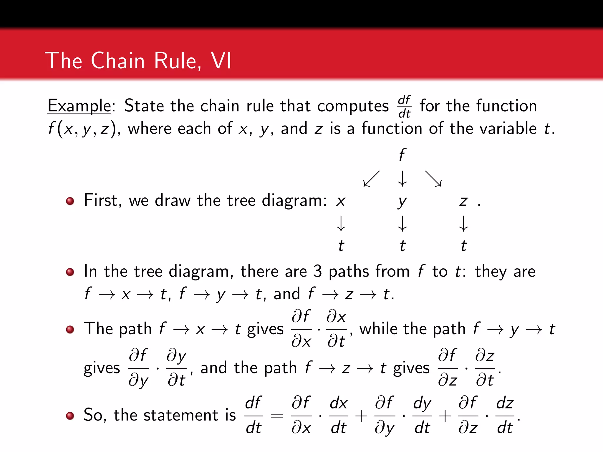
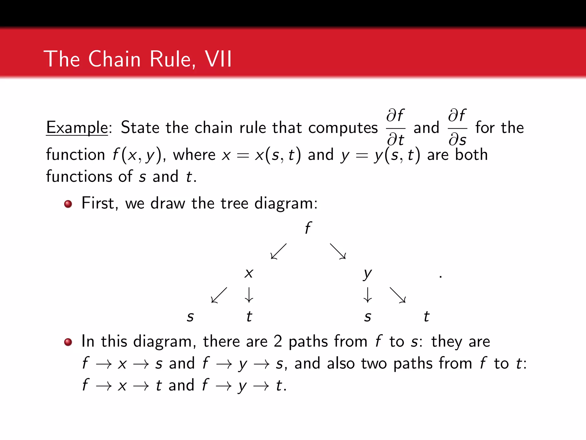
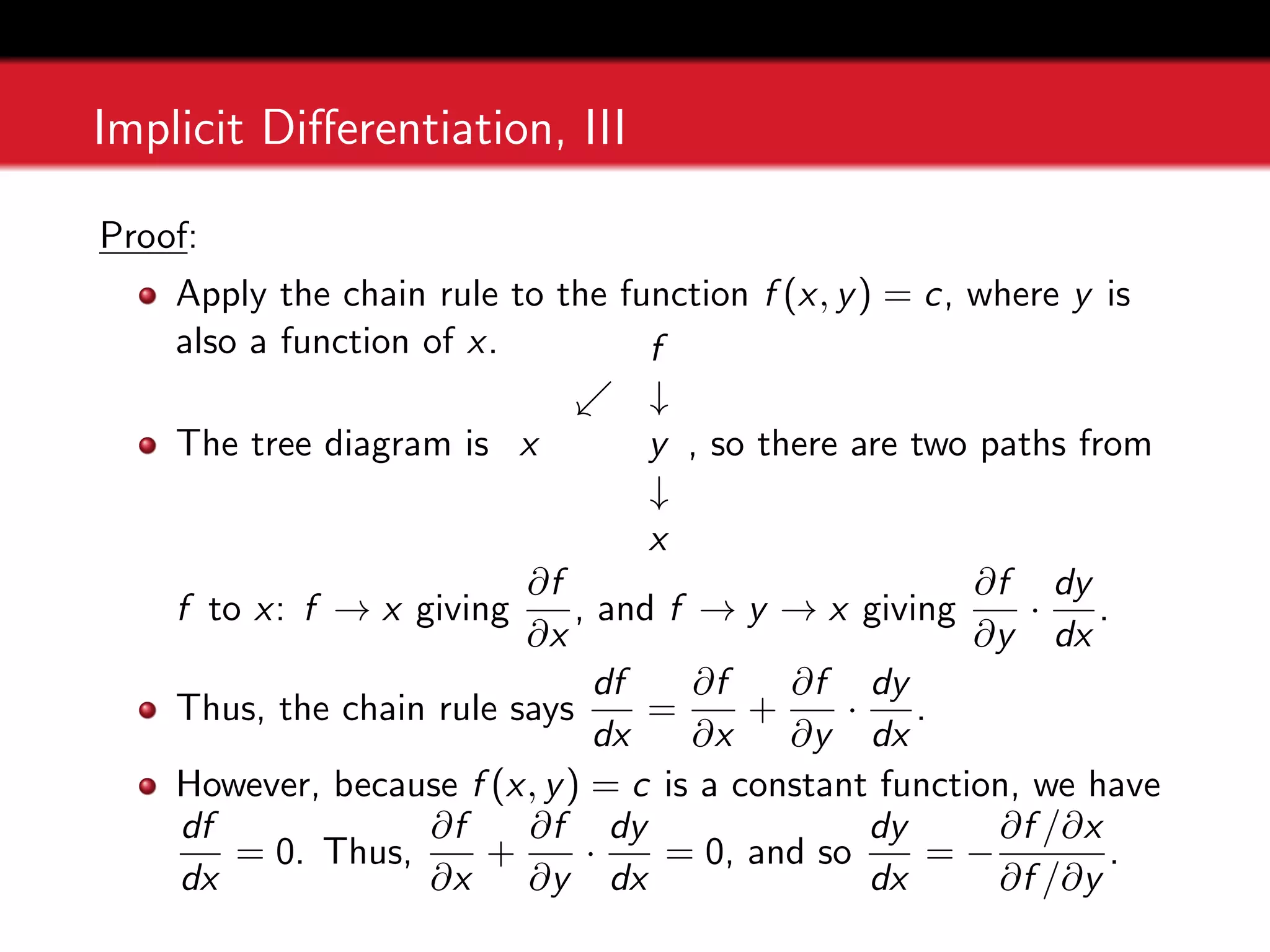
The method is to draw a “tree diagram” as follows:
1. Start with the initial function f , and draw an arrow pointing
from f to each of the variables it depends on.
2. For each variable listed, draw new arrows branching from that
variable to any other variables they depend on. Repeat the
process until all dependencies are shown in the diagram.
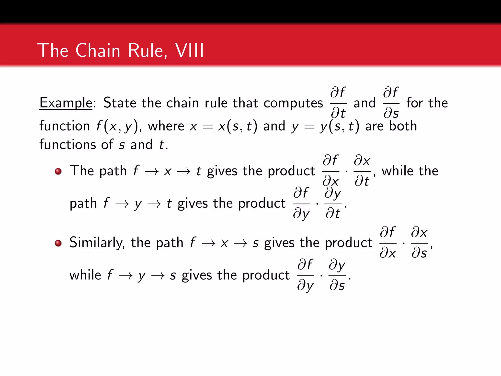
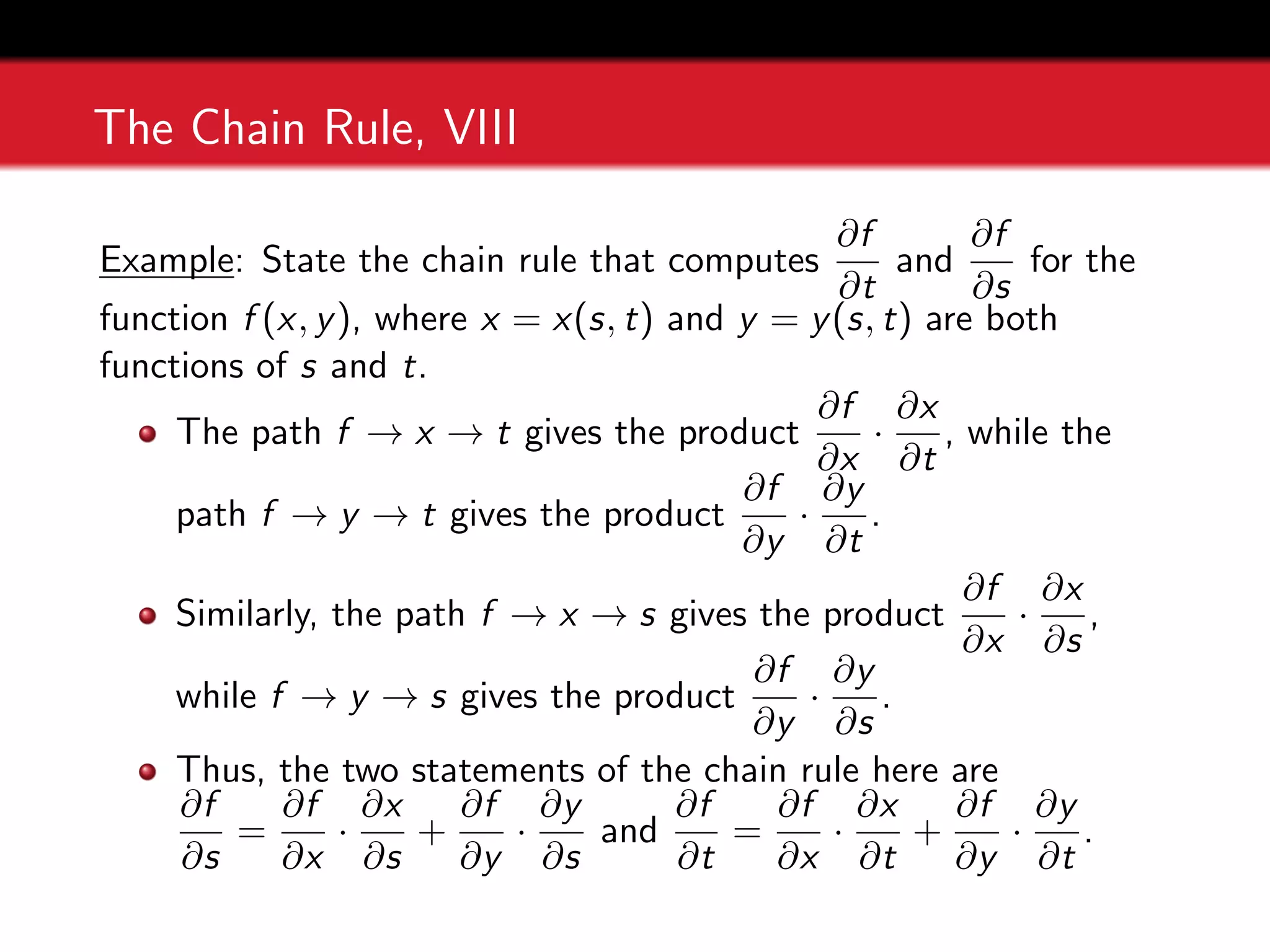
3. Associate each arrow from one variable to another with the
derivative
∂[top]
∂[bottom]
.
4. To write the version of the chain rule that gives the derivative
∂v1/∂v2 for any variables v1 and v2 in the diagram (where v2
depends on v1), first find all paths from v1 to v2.
5. For each path from v1 to v2, multiply all of the derivatives
that appear in each path from v1 to v2. Finally, sum the
results over all of the paths: this is ∂v1/∂v2.
12. The Chain Rule, VI
Example: State the chain rule that computes df
dt for the function
f (x, y, z), where each of x, y, and z is a function of the variable t.
13. The Chain Rule, VI
Example: State the chain rule that computes df
dt for the function
f (x, y, z), where each of x, y, and z is a function of the variable t.
First, we draw the tree diagram:
f
. ↓ &
x y z
↓ ↓ ↓
t t t
.
In the tree diagram, there are 3 paths from f to t: they are
f → x → t, f → y → t, and f → z → t.
The path f → x → t gives
∂f
∂x
·
∂x
∂t
, while the path f → y → t
gives
∂f
∂y
·
∂y
∂t
, and the path f → z → t gives
∂f
∂z
·
∂z
∂t
.
So, the statement is
df
dt
=
∂f
∂x
·
dx
dt
+
∂f
∂y
·
dy
dt
+
∂f
∂z
·
dz
dt
.
14. The Chain Rule, VII
Example: State the chain rule that computes df
dt for the function
f (x, y, z), where each of x, y, and z is a function of the variable t.
The chain rule says
df
dt
=
∂f
∂x
·
dx
dt
+
∂f
∂y
·
dy
dt
+
∂f
∂z
·
dz
dt
.
You can interpret this statement as saying that the total
change in f is the sum of three components:
1. The change
∂f
∂x
·
dx
dt
in f resulting from the change in x.
2. The change
∂f
∂y
·
dy
dt
in f resulting from the change in y.
3. The change
∂f
∂z
·
dz
dt
in f resulting from the change in z.
15. The Chain Rule, VII
Example: State the chain rule that computes
∂f
∂t
and
∂f
∂s
for the
function f (x, y), where x = x(s, t) and y = y(s, t) are both
functions of s and t.
16. The Chain Rule, VII
Example: State the chain rule that computes
∂f
∂t
and
∂f
∂s
for the
function f (x, y), where x = x(s, t) and y = y(s, t) are both
functions of s and t.
First, we draw the tree diagram:
f
. &
x y
. ↓ ↓ &
s t s t
.
In this diagram, there are 2 paths from f to s: they are
f → x → s and f → y → s, and also two paths from f to t:
f → x → t and f → y → t.
17. The Chain Rule, VIII
Example: State the chain rule that computes
∂f
∂t
and
∂f
∂s
for the
function f (x, y), where x = x(s, t) and y = y(s, t) are both
functions of s and t.
The path f → x → t gives the product
∂f
∂x
·
∂x
∂t
, while the
path f → y → t gives the product
∂f
∂y
·
∂y
∂t
.
Similarly, the path f → x → s gives the product
∂f
∂x
·
∂x
∂s
,
while f → y → s gives the product
∂f
∂y
·
∂y
∂s
.
18. The Chain Rule, VIII
Example: State the chain rule that computes
∂f
∂t
and
∂f
∂s
for the
function f (x, y), where x = x(s, t) and y = y(s, t) are both
functions of s and t.
The path f → x → t gives the product
∂f
∂x
·
∂x
∂t
, while the
path f → y → t gives the product
∂f
∂y
·
∂y
∂t
.
Similarly, the path f → x → s gives the product
∂f
∂x
·
∂x
∂s
,
while f → y → s gives the product
∂f
∂y
·
∂y
∂s
.
Thus, the two statements of the chain rule here are
∂f
∂s
=
∂f
∂x
·
∂x
∂s
+
∂f
∂y
·
∂y
∂s
and
∂f
∂t
=
∂f
∂x
·
∂x
∂t
+
∂f
∂y
·
∂y
∂t
.
19. The Chain Rule, IX
Example: For f (x, y) = x2 + y2, with x = t2 and y = t4, find
df
dt
,
both directly and via the chain rule.
20. The Chain Rule, IX
Example: For f (x, y) = x2 + y2, with x = t2 and y = t4, find
df
dt
,
both directly and via the chain rule.
In this instance, the multivariable chain rule says that
df
dt
=
∂f
∂x
·
dx
dt
+
∂f
∂y
·
dy
dt
.
Computing the derivatives shows
df
dt
= (2x) · (2t) + (2y) · (4t3).
Plugging in x = t2 and y = t4 yields
df
dt
= (2t2) · (2t) + (2t4) · (4t3) = 4t3 + 8t7.
To do this directly, we would plug in x = t2 and y = t4: this
gives f (x, y) = t4 + t8, so that
df
dt
= 4t3 + 8t7.
Of course, we obtain the same answer either way!
21. The Chain Rule, X
Example: Let f (x, y) = x2 + y2, where x = s2 + t2 and
y = s3 + t4.
1. Find
∂f
∂s
. 2. Find
∂f
∂t
.
22. The Chain Rule, X
Example: Let f (x, y) = x2 + y2, where x = s2 + t2 and
y = s3 + t4.
1. Find
∂f
∂s
. 2. Find
∂f
∂t
.
We just need to write down and then apply the appropriate
version of the chain rule.
23. The Chain Rule, XI
Example: Let f (x, y) = x2 + y2, where x = s2 + t2 and
y = s3 + t4.
1. Find
∂f
∂s
.
24. The Chain Rule, XI
Example: Let f (x, y) = x2 + y2, where x = s2 + t2 and
y = s3 + t4.
1. Find
∂f
∂s
.
By the chain rule we have
∂f
∂s
=
∂f
∂x
·
∂x
∂s
+
∂f
∂y
·
∂y
∂s
= (2x) · (2s) + (2y) · (3s2).
Plugging in x = s2 + t2 and y = s3 + t4 yields
∂f
∂s
= (2s2
+ 2t2
) · (2s) + (2s3
+ 2t4
) · (3s2
)
= 4s3
+ 4st2
+ 6s5
+ 6s2
t4
.
25. The Chain Rule, XII
Example: Let f (x, y) = x2 + y2, where x = s2 + t2 and
y = s3 + t4.
2. Find
∂f
∂t
.
26. The Chain Rule, XII
Example: Let f (x, y) = x2 + y2, where x = s2 + t2 and
y = s3 + t4.
2. Find
∂f
∂t
.
By the chain rule we have
∂f
∂t
=
∂f
∂x
·
∂x
∂t
+
∂f
∂y
·
∂y
∂t
= (2x) · (2t) + (2y) · (4t3).
Plugging in x = s2 + t2 and y = s3 + t4 yields
∂f
∂s
= (2s2
+ 2t2
) · (2t) + (2s3
+ 2t4
) · (4t3
)
= 4s2
t + 4t3
+ 8s3
t3
+ 8t7
.
27. The Chain Rule, Lucky XIII
Example: Suppose x and y are functions of s and t with
x(1, 5) = 2, y(1, 5) = −2, and that f has partial derivatives below.
∂f
∂x
(1, 5) = 7
∂f
∂y
(1, 5) = −6
∂f
∂x
(2, −2) = 1
∂f
∂y
(2, −2) = −4
∂x
∂s
(1, 5) = 3
∂x
∂t
(1, 5) = 2
∂y
∂s
(1, 5) = 4
∂y
∂t
(1, 5) = −2
1. Find
∂f
∂s
at (s, t) = (1, 5). 2. Find
∂f
∂t
at (s, t) = (1, 5).
28. The Chain Rule, Lucky XIII
Example: Suppose x and y are functions of s and t with
x(1, 5) = 2, y(1, 5) = −2, and that f has partial derivatives below.
∂f
∂x
(1, 5) = 7
∂f
∂y
(1, 5) = −6
∂f
∂x
(2, −2) = 1
∂f
∂y
(2, −2) = −4
∂x
∂s
(1, 5) = 3
∂x
∂t
(1, 5) = 2
∂y
∂s
(1, 5) = 4
∂y
∂t
(1, 5) = −2
1. Find
∂f
∂s
at (s, t) = (1, 5). 2. Find
∂f
∂t
at (s, t) = (1, 5).
This problem is an application of the chain rule. We need only
write down the appropriate chain rule and then plug in the
proper values (namely, s = 1 and t = 5).
However, the notation for this problem is tricky. The variables
for f are x and y, and when s = 1 and t = 5, we have x = 2
and y = −2. So we want to use the two entries on the top
right, not the top left.
29. The Chain Rule, XIV
Example: Suppose x and y are functions of s and t with
x(1, 5) = 2, y(1, 5) = −2, and that f has partial derivatives below.
∂f
∂x
(1, 5) = 7
∂f
∂y
(1, 5) = −6
∂f
∂x
(2, −2) = 1
∂f
∂y
(2, −2) = −4
∂x
∂s
(1, 5) = 3
∂x
∂t
(1, 5) = 2
∂y
∂s
(1, 5) = 4
∂y
∂t
(1, 5) = −2
1. Find
∂f
∂s
at (s, t) = (1, 5).
30. The Chain Rule, XIV
Example: Suppose x and y are functions of s and t with
x(1, 5) = 2, y(1, 5) = −2, and that f has partial derivatives below.
∂f
∂x
(1, 5) = 7
∂f
∂y
(1, 5) = −6
∂f
∂x
(2, −2) = 1
∂f
∂y
(2, −2) = −4
∂x
∂s
(1, 5) = 3
∂x
∂t
(1, 5) = 2
∂y
∂s
(1, 5) = 4
∂y
∂t
(1, 5) = −2
1. Find
∂f
∂s
at (s, t) = (1, 5).
By the chain rule,
∂f
∂s
=
∂f
∂x
·
∂x
∂s
+
∂f
∂y
·
∂y
∂s
.
Setting (s, t) = (1, 5) and noting that x(1, 5) = 2,
y(1, 5) = −2 yields
∂f
∂s
(1, 5) = 1 · 3 + (−4) · 4 = −13.
31. The Chain Rule, XV
Example: Suppose x and y are functions of s and t with
x(1, 5) = 2, y(1, 5) = −2, and that f has partial derivatives below.
∂f
∂x
(1, 5) = 7
∂f
∂y
(1, 5) = −6
∂f
∂x
(2, −2) = 1
∂f
∂y
(2, −2) = −4
∂x
∂s
(1, 5) = 3
∂x
∂t
(1, 5) = 2
∂y
∂s
(1, 5) = 4
∂y
∂t
(1, 5) = −2
2. Find
∂f
∂t
at (s, t) = (1, 5).
32. The Chain Rule, XV
Example: Suppose x and y are functions of s and t with
x(1, 5) = 2, y(1, 5) = −2, and that f has partial derivatives below.
∂f
∂x
(1, 5) = 7
∂f
∂y
(1, 5) = −6
∂f
∂x
(2, −2) = 1
∂f
∂y
(2, −2) = −4
∂x
∂s
(1, 5) = 3
∂x
∂t
(1, 5) = 2
∂y
∂s
(1, 5) = 4
∂y
∂t
(1, 5) = −2
2. Find
∂f
∂t
at (s, t) = (1, 5).
By the chain rule,
∂f
∂t
=
∂f
∂x
·
∂x
∂t
+
∂f
∂y
·
∂y
∂t
.
Setting (s, t) = (1, 5) and noting that x(1, 5) = 2,
y(1, 5) = −2 yields
∂f
∂t
(1, 5) = 1 · 2 + (−4) · (−2) = 10.
33. The Chain Rule, XVI
Example: Suppose f (x, y, z) is a function of x, y, z, where z is a
function of x and t, and x and y are also both functions of t.
1. State the chain rule for finding
df
dt
.
34. The Chain Rule, XVI
Example: Suppose f (x, y, z) is a function of x, y, z, where z is a
function of x and t, and x and y are also both functions of t.
1. State the chain rule for finding
df
dt
.
We just need to write down and then apply the
appropriate version of the chain rule.
Drawing the tree diagram yields paths f → x → t,
f → y → t, f → z → x → t, and f → z → t.
Thus, the statement is
df
dt
=
∂f
∂x
dx
dt
+
∂f
∂y
dy
dt
+
∂f
∂z
∂z
∂x
dx
dt
+
∂f
∂z
∂z
∂t
.
2. Try it for f (x, y, z) = x2 + y3 + z4, x = t2, y = t3, z = x2t.
35. The Chain Rule, XVI
Example: Suppose f (x, y, z) is a function of x, y, z, where z is a
function of x and t, and x and y are also both functions of t.
1. State the chain rule for finding
df
dt
.
We just need to write down and then apply the
appropriate version of the chain rule.
Drawing the tree diagram yields paths f → x → t,
f → y → t, f → z → x → t, and f → z → t.
Thus, the statement is
df
dt
=
∂f
∂x
dx
dt
+
∂f
∂y
dy
dt
+
∂f
∂z
∂z
∂x
dx
dt
+
∂f
∂z
∂z
∂t
.
2. Try it for f (x, y, z) = x2 + y3 + z4, x = t2, y = t3, z = x2t.
df /dt = (2x)(2t) + (3y2)(3t2) + (4z3)(2xt)(2t) + (4z3)(x2).
36. The Chain Rule, XVII
Amusingly, we can actually derive the other differentiation rules
using the (multivariable) chain rule!
To obtain the product rule, let P(f , g) = fg, where f and g
are both functions of x.
Then the chain rule says
dP
dx
=
∂P
∂f
·
df
dx
+
∂P
∂g
·
dg
dx
= g ·
df
dx
+ f ·
dg
dx
.
If we rewrite this expression using single-variable notation, it
reads as the more familiar (fg)0 = f 0g + fg0, which is, indeed,
the product rule.
Likewise, if we set Q(f , g) = f /g where f and g are both
functions of x, then applying the chain rule gives
dQ
dx
=
∂Q
∂f
·
df
dx
+
∂Q
∂g
·
dg
dx
=
1
g
·
df
dx
−
f
g2
·
dg
dx
=
f 0g − fg0
g2
;
this is the quotient rule.
37. Implicit Differentiation, I
Using the chain rule for several variables, we can give an
alternative way to solve problems involving implicit differentiation
from calculus of a single variable.
A typical example is as follows: if y is defined implicitly by
x3y2 + sin(2xy) = 7, find the derivative y0 = dy/dx.
To solve this problem one differentiates both sides with
respect to x, using the chain rule to differentiate any terms
involving y, and then solves for y0.
This yields 3x2y2 + x3(2yy0) + (2y + 2xy0) cos(2xy) = 0, so
that y0 = −
3x2y2 + 2y cos(2xy)
2x3y + 2x cos(2xy)
.
Although there is nothing conceptually difficult about this
problem, it is often very easy to make algebra mistakes.
However, implicit differentiation is actually very simple and
straightforward if we use partial derivatives.
38. Implicit Differentiation, II
Here is how to do implicit differentiation with partial derivatives:
Theorem (Implicit Differentiation)
Given an implicit relation f (x, y) = c, the implicit single-variable
derivative
dy
dx
= y0(x) is given by
dy
dx
= −
∂f /∂x
∂f /∂y
= −
fx
fy
.
The key idea behind this formula is to invoke the multivariable
chain rule on the implicit relation f (x, y) = c, where we think of y
as being a function of x.
39. Implicit Differentiation, III
Proof:
Apply the chain rule to the function f (x, y) = c, where y is
also a function of x.
The tree diagram is
f
. ↓
x y
↓
x
, so there are two paths from
f to x: f → x giving
∂f
∂x
, and f → y → x giving
∂f
∂y
·
dy
dx
.
Thus, the chain rule says
df
dx
=
∂f
∂x
+
∂f
∂y
·
dy
dx
.
However, because f (x, y) = c is a constant function, we have
df
dx
= 0. Thus,
∂f
∂x
+
∂f
∂y
·
dy
dx
= 0, and so
dy
dx
= −
∂f /∂x
∂f /∂y
.
41. Implicit Differentiation, IV
Example: If y is defined implicitly by x3y2 + sin(2xy) = 7, find the
derivative y0 = dy/dx.
This is the relation f (x, y) = 7 for f (x, y) = x3y2 + sin(2xy).
We have fx = 3x2y2 + 2y cos(2xy) and
fy = 2x3y + 2x cos(2xy).
So, the formula gives y0 =
dy
dx
= −
3x2y2 + 2y cos(2xy)
2x3y + 2x cos(2xy)
.
Note that this agrees with the implicit differentiation
calculation I did a few slides ago. (You can decide for yourself
which one seems easier!)
43. Implicit Differentiation, V
Example: Find y0, if y2x3 + y ex = 2.
This is the relation f (x, y) = 2, where f (x, y) = y2x3 + y ex .
We have fx = 3y2x2 + y ex , and fy = 2yx3 + ex , so the
formula gives y0 =
dy
dx
= −
fx
fy
= −
3y2x2 + y ex
2yx3 + ex
.
If you want to check this by doing the implicit differentiation
directly, here is the calculation:
We have
d
dx
y2x3 + y ex
= 0.
Differentiating the left-hand side yields
2yy0x3 + 3y2x2
+ (y0 ex + y ex ) = 0.
Rearranging yields 2yx3 + ex
y0 + 3y2x2 + y ex
= 0.
So y0 = −
3y2x2 + y ex
2yx3 + ex
.
44. Implicit Differentiation, VI
We can also perform implicit differentiation in the event that there
are more than 2 variables.
For an implicit relation f (x, y, z) = c, we can compute
implicit derivatives for any of the 3 variables with respect to
either of the others, using a chain rule calculation like in the
theorem earlier.
45. Implicit Differentiation, VII
The idea is simply to view any variables other than our target
variables as constants.
So, if we have an implicit relation f (x, y, z) = c and want to
compute
∂z
∂x
, we view the other variable (in this case y) as
constant. Then the chain rule says
∂z
∂x
= −
∂f /∂x
∂f /∂z
= −
fx
fz
.
If we wanted to compute
∂z
∂y
then we would view x as a
constant, and then
∂z
∂y
= −
∂f /∂y
∂f /∂z
= −
fy
fz
.
Similarly,
∂y
∂x
= −
fx
fy
,
∂y
∂z
= −
fz
fy
,
∂x
∂y
= −
fy
fx
, and
∂x
∂z
= −
fz
fx
.
The general form is
∂v
∂w
= −
fw
fv
for any variables v, w.
47. Implicit Differentiation, VIII
Example: Suppose that x, y, z satisfy x2yz + ex cos(y) = 3.
1. If z is defined implicitly in terms of x and y, find ∂z/∂x.
The implicit relation is f (x, y, z) = 3 where
f (x, y, z) = x2yz + ex cos(y). We then compute
fx = 2xyz + ex cos(y), fy = x2z − ex sin(y), fz = x2y.
By the implicit differentiation formulas,
∂z
∂x
= −
∂f /∂x
∂f /∂z
= −
fx
fz
= −
2xyz + ex cos(y)
x2y
.
2. If y is defined implicitly in terms of x and z, find ∂y/∂z.
48. Implicit Differentiation, VIII
Example: Suppose that x, y, z satisfy x2yz + ex cos(y) = 3.
1. If z is defined implicitly in terms of x and y, find ∂z/∂x.
The implicit relation is f (x, y, z) = 3 where
f (x, y, z) = x2yz + ex cos(y). We then compute
fx = 2xyz + ex cos(y), fy = x2z − ex sin(y), fz = x2y.
By the implicit differentiation formulas,
∂z
∂x
= −
∂f /∂x
∂f /∂z
= −
fx
fz
= −
2xyz + ex cos(y)
x2y
.
2. If y is defined implicitly in terms of x and z, find ∂y/∂z.
Using the calculations above, we get
∂y
∂z
= −
∂f /∂z
∂f /∂y
= −
fz
fy
= −
x2y
x2z − ex sin(y)
.
49. Summary
We introduced the multivariable chain rule and discussed how to
apply it.
We discussed implicit differentiation using the multivariable chain
rule.
Next lecture: Minima and maxima, classification of critical points.