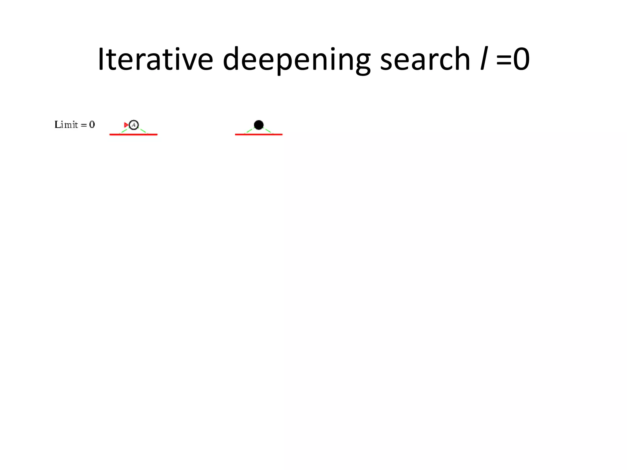
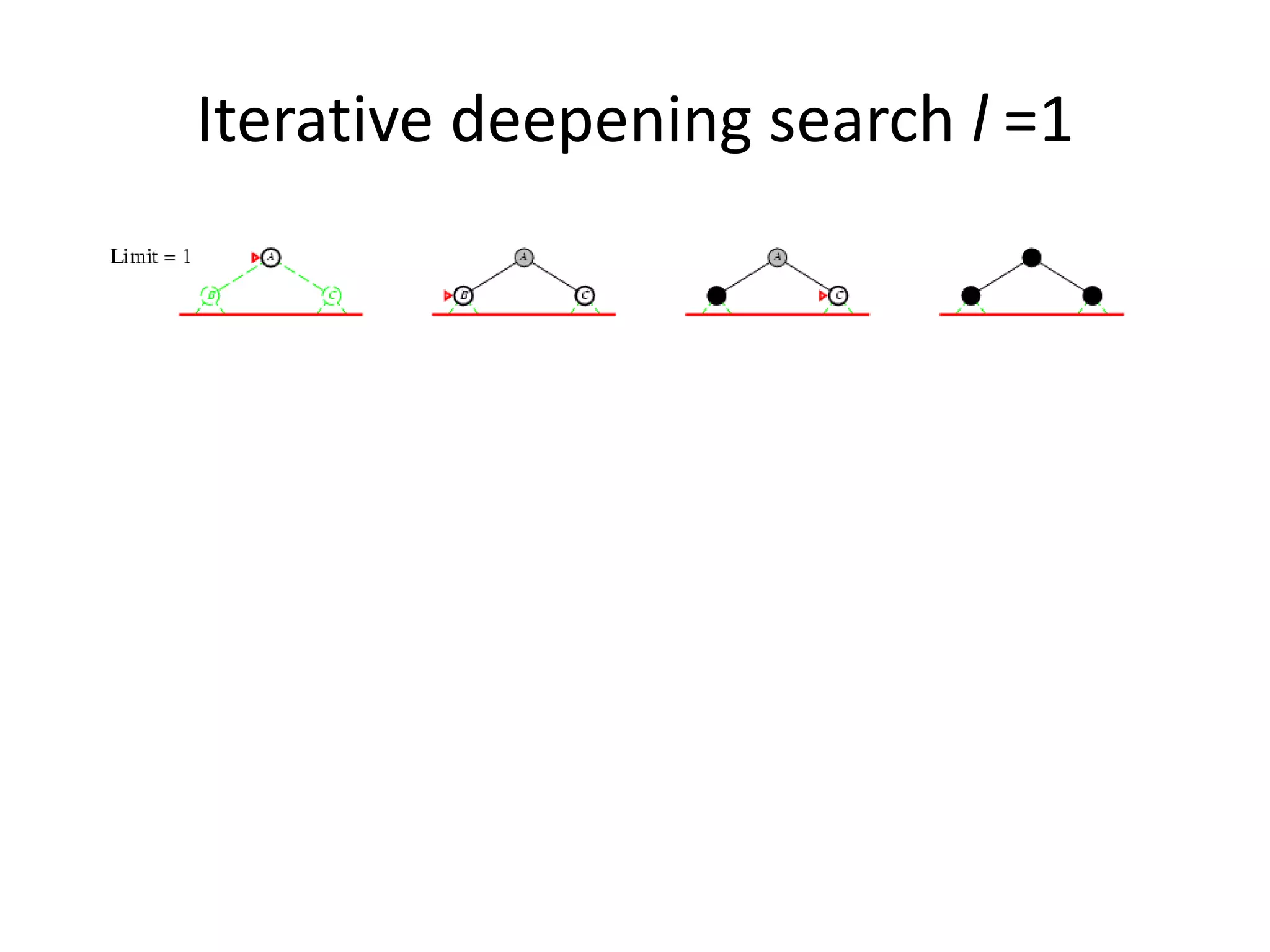
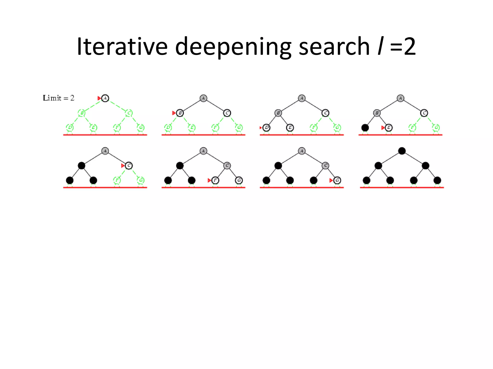
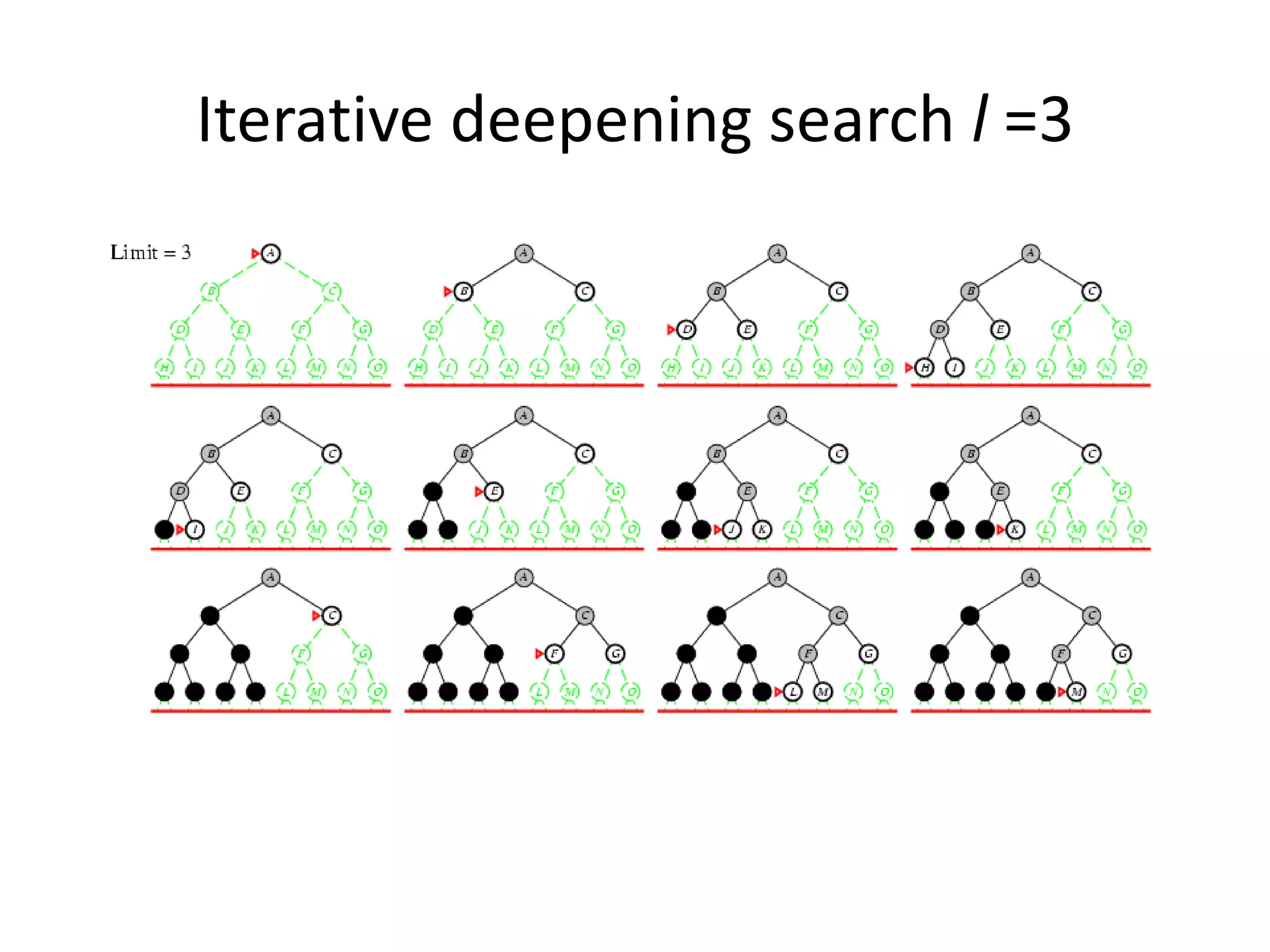
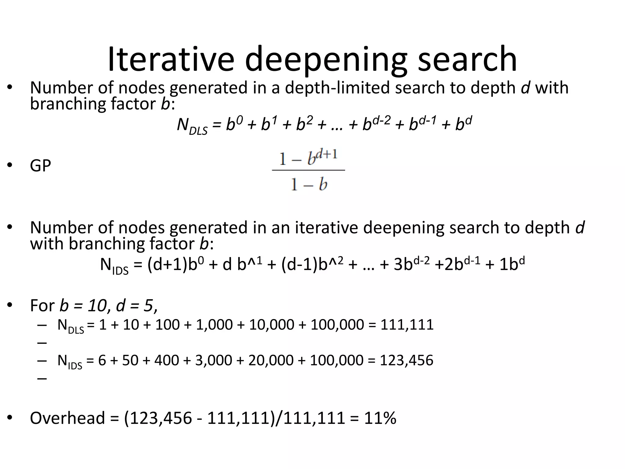
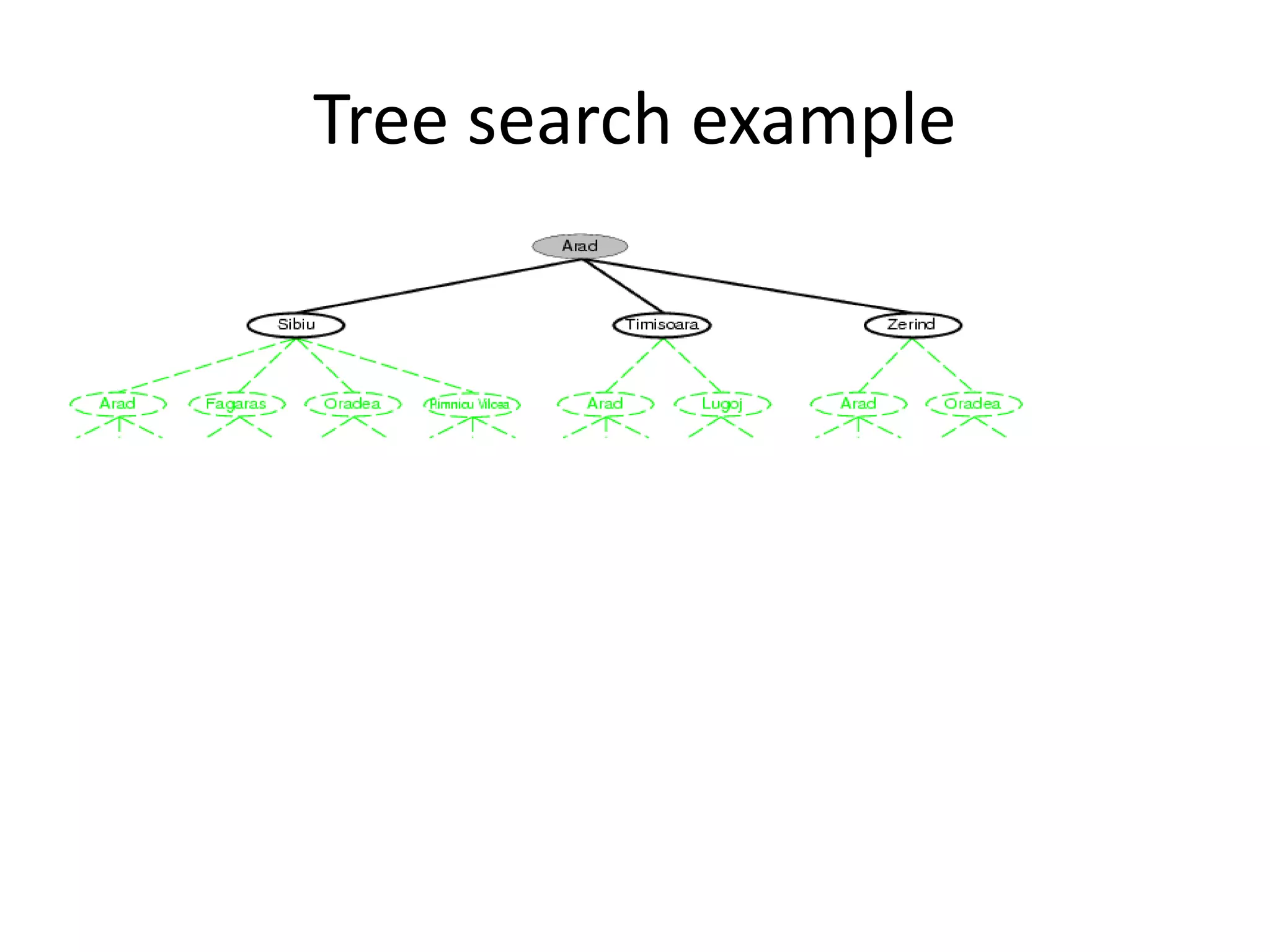
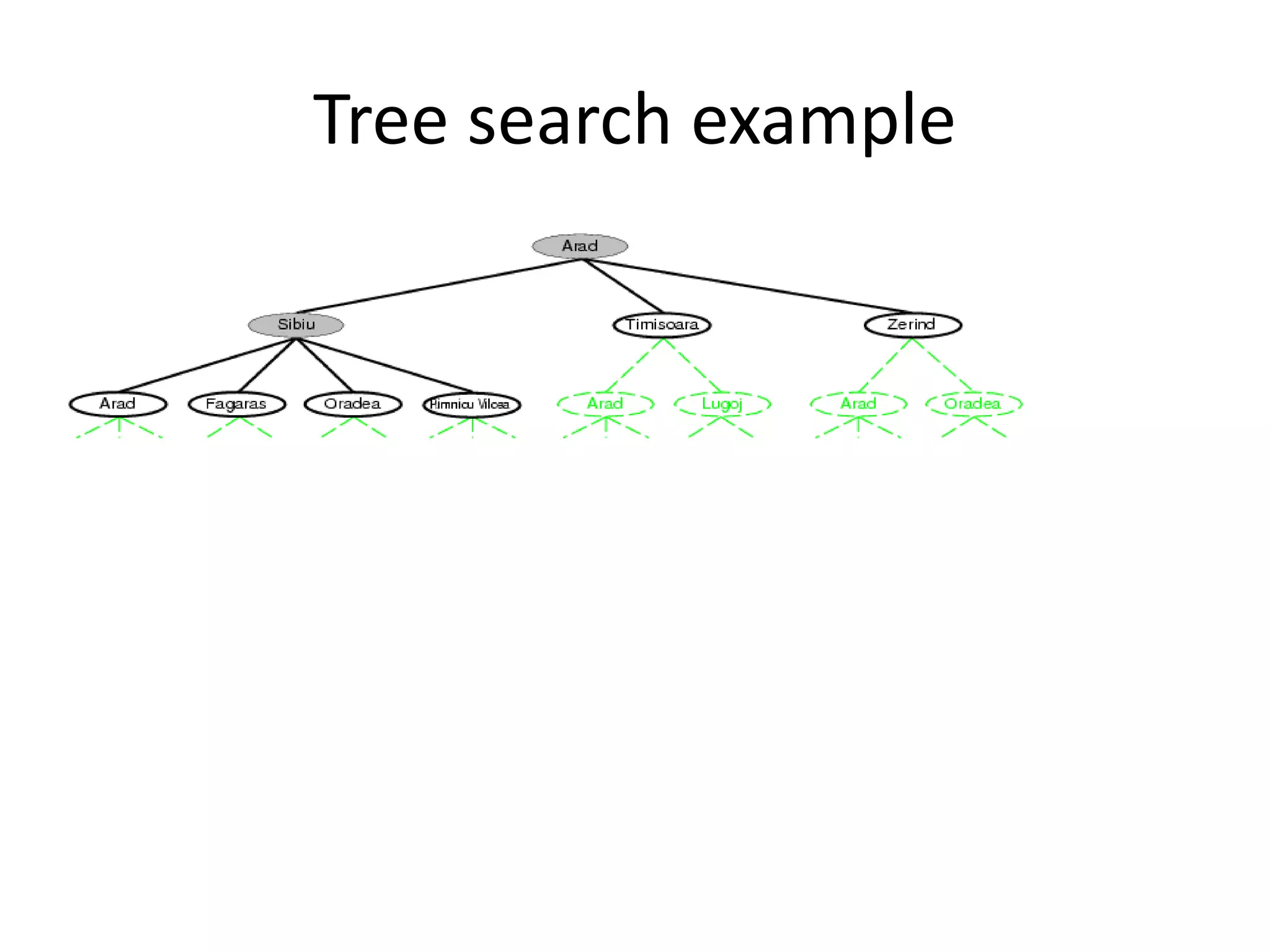
The document discusses different search algorithms used in artificial intelligence including depth-first search, breadth-first search, and iterative deepening search. It provides details on how each algorithm works, including that depth-first search puts successors at the front of a queue, breadth-first search puts successors at the end of a queue, and iterative deepening search performs repeated depth-limited searches with increasing depth limits. Examples are given to illustrate tree search and the different search strategies.

1. Lecture 3
Note: Some slides and/or pictures are adapted from Lecture slides / Books of
• Dr Zafar Alvi.
• Text Book - Aritificial Intelligence Illuminated by Ben Coppin, Narosa Publishers.
• Ref Books
•Artificial Intelligence- Structures & Strategies for Complex Problem Solving by George F. Luger, 4th edition,
Pearson Education.
• Artificial Intelligence A Modern Approach by Stuart Russell & Peter Norvig.
•Artificial Intelligence, Third Edition by Patrick Henry Winston

2. Outline
• Problems and their representation
• Goal Driven VS Data Driven
• Properties of search Methods
• Tree search algorithm
– Depth First algorithm
– Breadth First algorithm
– Iterative Deepening algorithm

3. Problems and their Representations
• Three men and three lions are on one side of a
river, with a boat. They all want to get to the
other side of the river. The boat can only hold
one or two at a time. At no time should there
be more lions than men on either side of the
river, as this would probably result in the men
being eaten.
• Representation could be 3, 3, 1 0, 0, 0

4. Problems and their Representations
• Traveling Salesman problem (NP complete)

5. Problems and their Representations
• Traversing a Maze

6. Data Driven or Goal Driven Search
• Data-driven search starts from an initial state
and uses actions that are allowed to move
forward until a goal is reached. This approach
is also known as forward chaining.
• Search can start at the goal and work back
toward a start state, by seeing what moves
could have led to the goal state. This is goal-
driven search, also known as backward
chaining.

7. Properties of Search Methods
• Complexity
• Completeness
• Optimality
• Admissibility
• Irrevocability

8. Complexity
• It is useful to describe how efficient that
method is, over time and space.
• The time complexity of a method is related to
the length of time that the method would take
to find a goal state.
• The space complexity is related to the amount
of memory that the method needs to use.

9. Completeness
• A search method is described as being
complete if it is guaranteed to find a goal state
if one exists.
• A method that is not complete has the
disadvantage that it cannot necessarily be
believed if it reports that no solution exists.

10. Optimality
• A search method is optimal if it finds a
solution in the quickest possible time.

11. Admissibility
• An algorithm is then defined as admissible if it
is guaranteed to find the best solution.

12. Irrevocability
• Methods that do not use backtracking, and
which therefore examine just one path, are
described as irrevocable.
• Irrevocable search methods will often find
suboptimal solutions to problems because
they tend to be fooled by local optima—
solutions that look good locally but are less
favorable when compared with other
solutions elsewhere in the search space.

13. Tree search algorithms
• Basic idea:
– offline, simulated exploration of state space by generating
successors of already-explored

14. Tree search example

15. Tree search example

16. Tree search example

17. Uninformed search strategies
• Uninformed search strategies use only the
information available in the problem
definition
– Depth-first search
– Breadth-first search
– Iterative deepening search
– etc

18. Depth-first search
• Expand deepest unexpanded node
• Implementation:
– put successors at front
–

19. Depth-first search
• Expand deepest unexpanded node
• Implementation:
– put successors at front
–

20. Depth-first search
• Expand deepest unexpanded node
• Implementation:
– put successors at front
–

21. Depth-first search
• Expand deepest unexpanded node
• Implementation:
– put successors at front
–

22. Depth-first search
• Expand deepest unexpanded node
• Implementation:
– put successors at front
–

23. Depth-first search
• Expand deepest unexpanded node
• Implementation:
– fringe = LIFO queue, i.e., put successors at front
–

24. Depth-first search
• Expand deepest unexpanded node
• Implementation:
– fringe = LIFO queue, i.e., put successors at front
–

25. Depth-first search
• Expand deepest unexpanded node
• Implementation:
– put successors at front
–

26. Depth-first search
• Expand deepest unexpanded node
• Implementation:
– put successors at front
–

27. Depth-first search
• Expand deepest unexpanded node
• Implementation:
– put successors at front
–

28. Depth-first search
• Expand deepest unexpanded node
• Implementation:
– put successors at front
–

29. Depth-first search
• Expand deepest unexpanded node
• Implementation:
– put successors at front
–

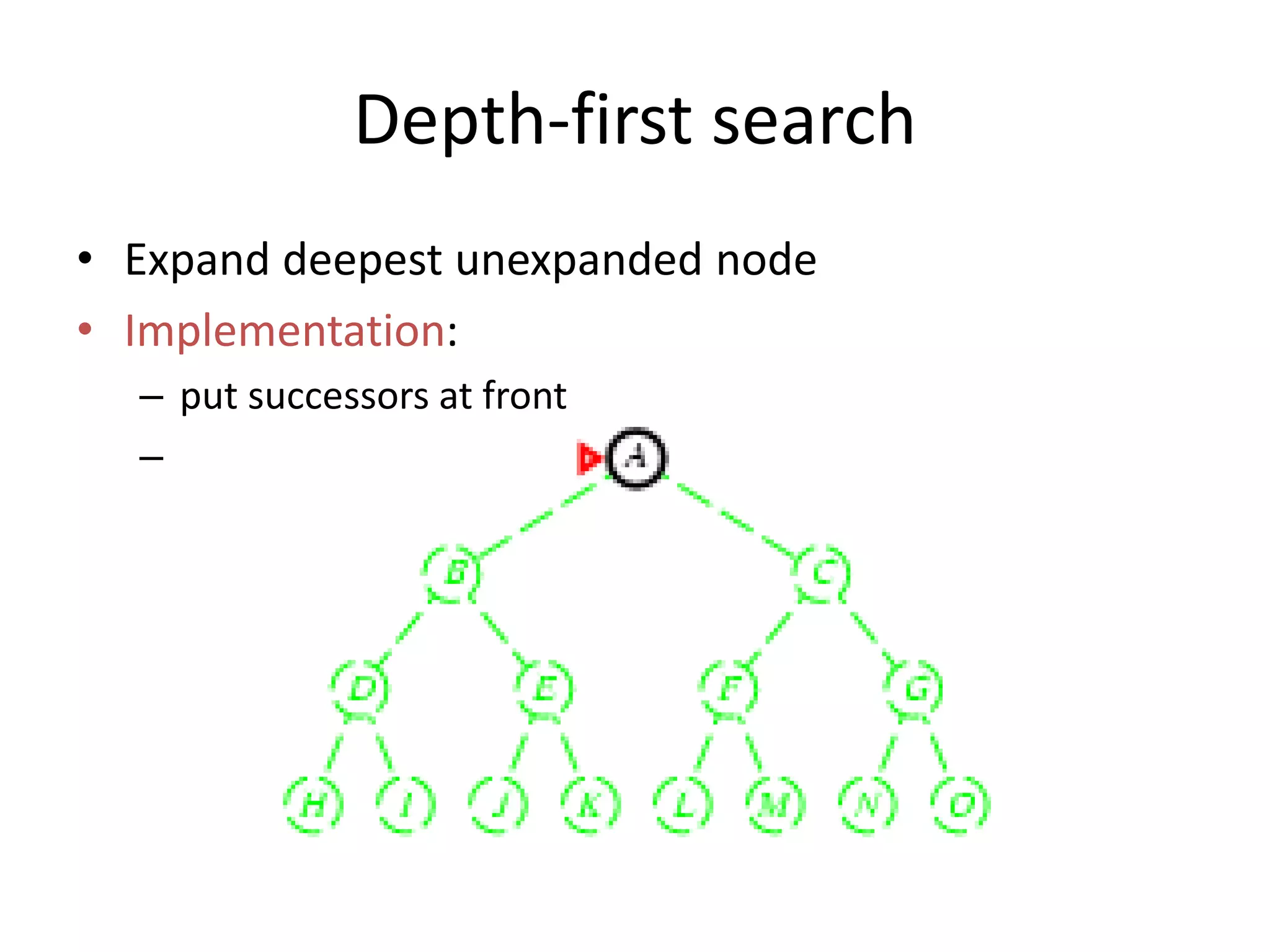
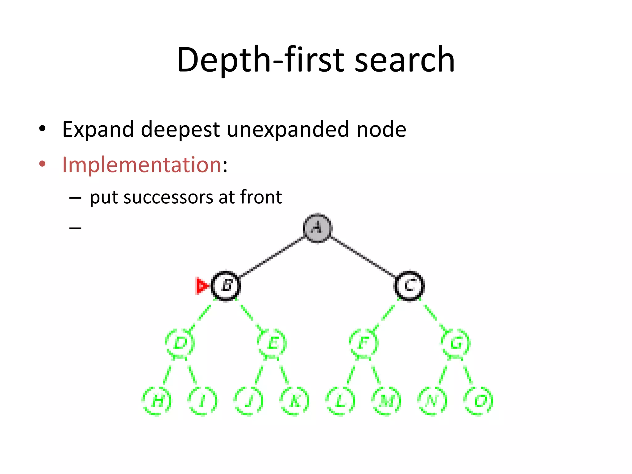
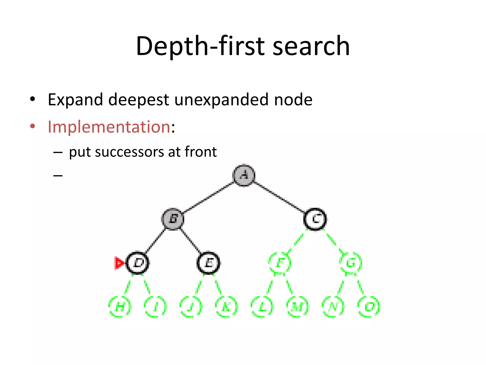
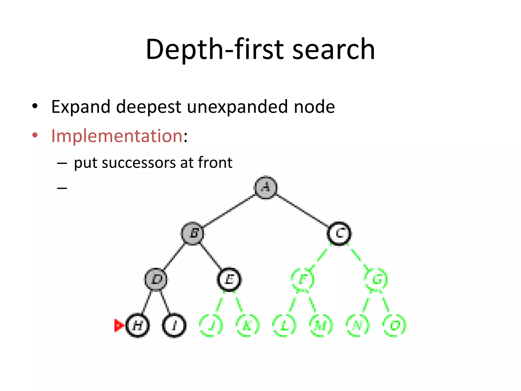
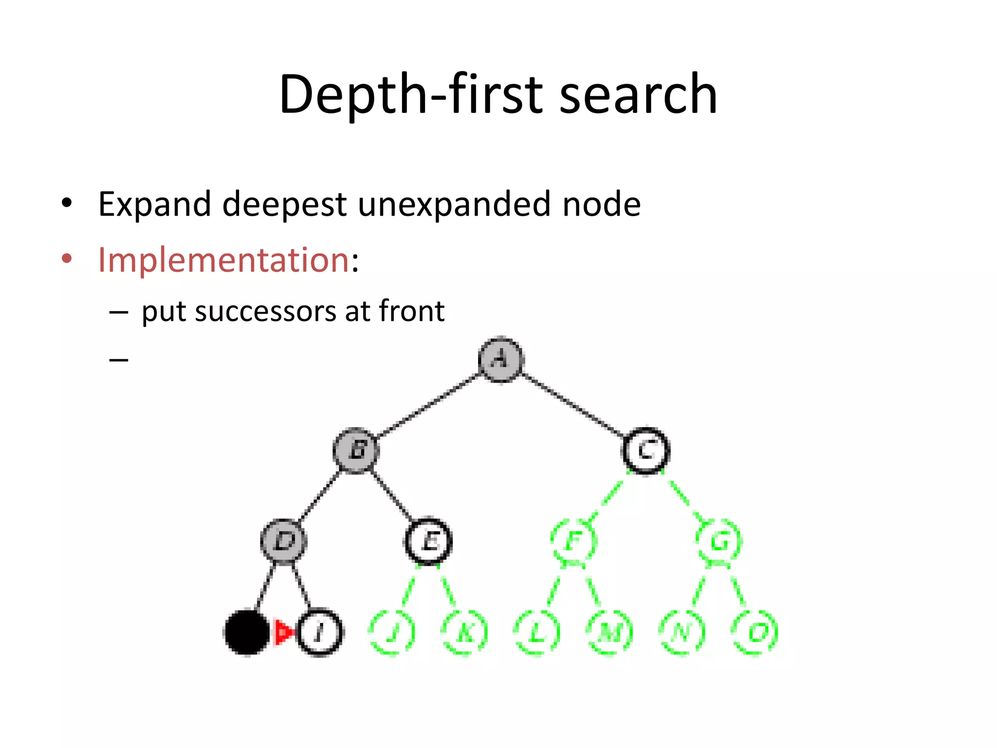
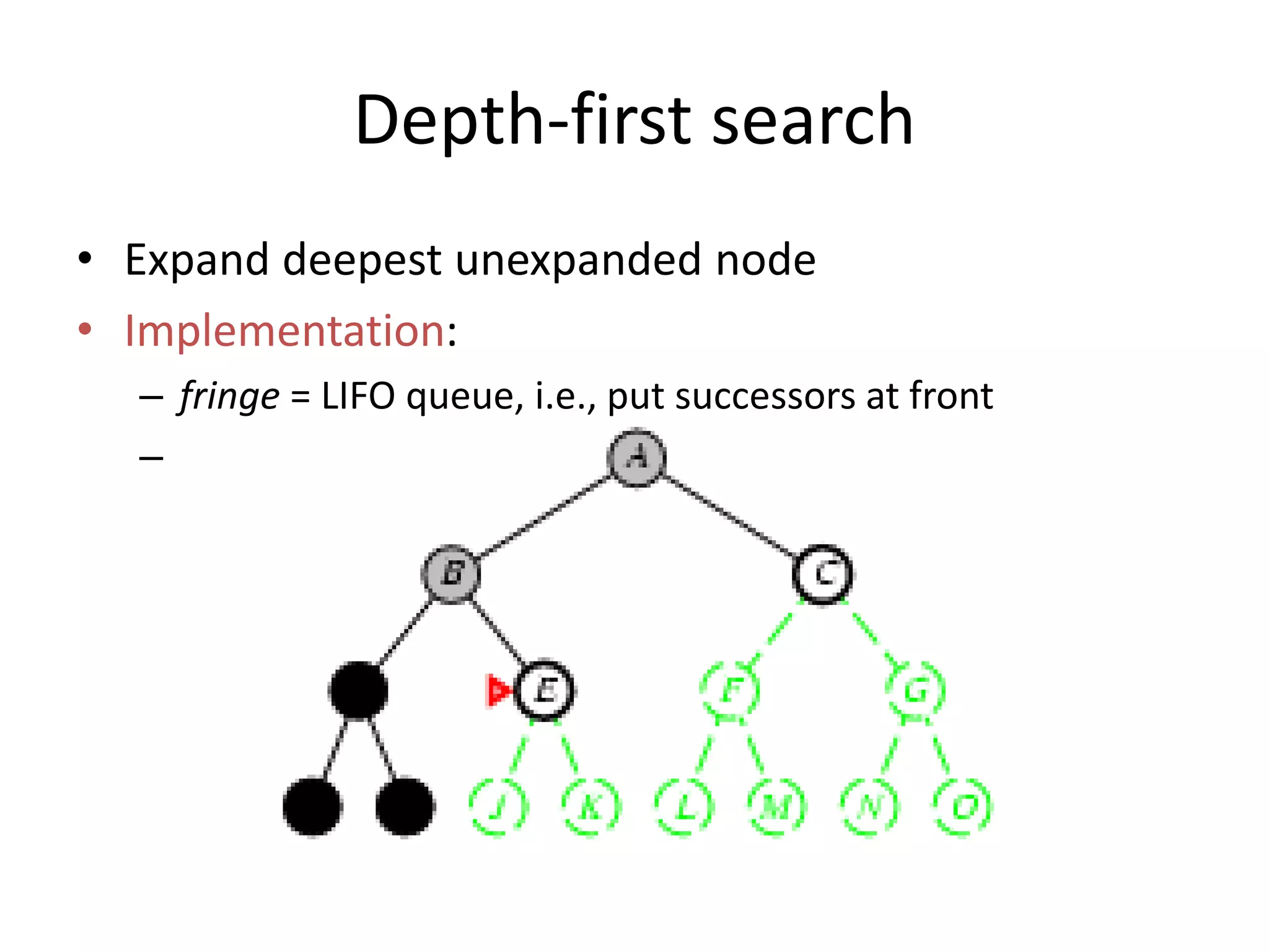
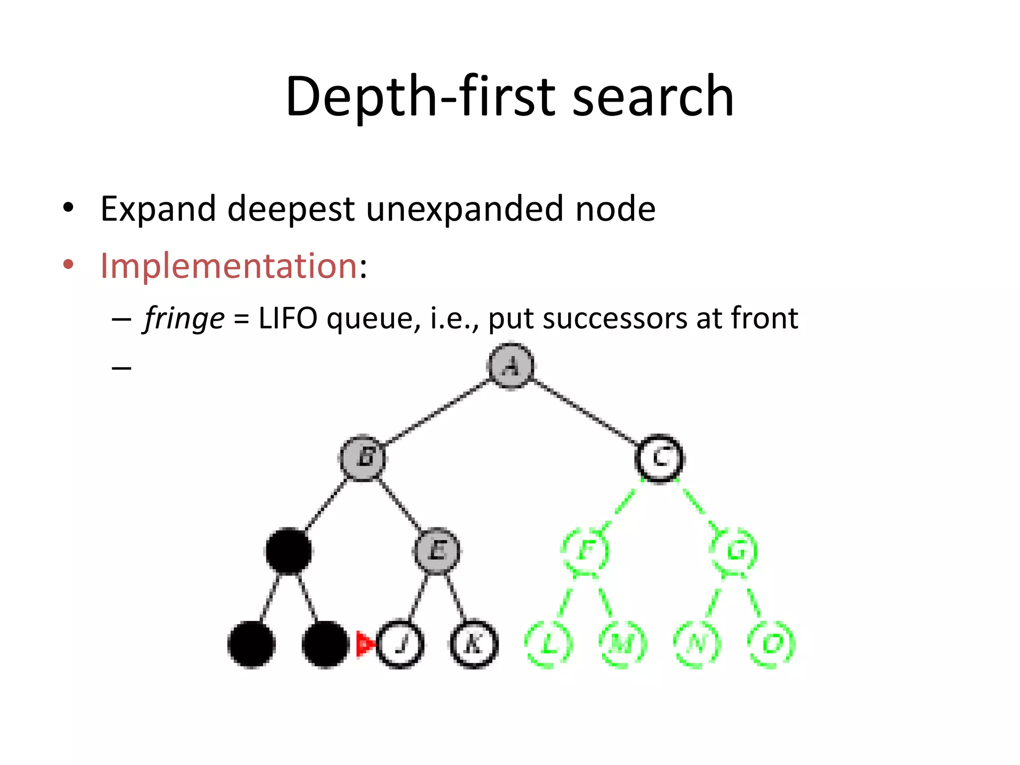
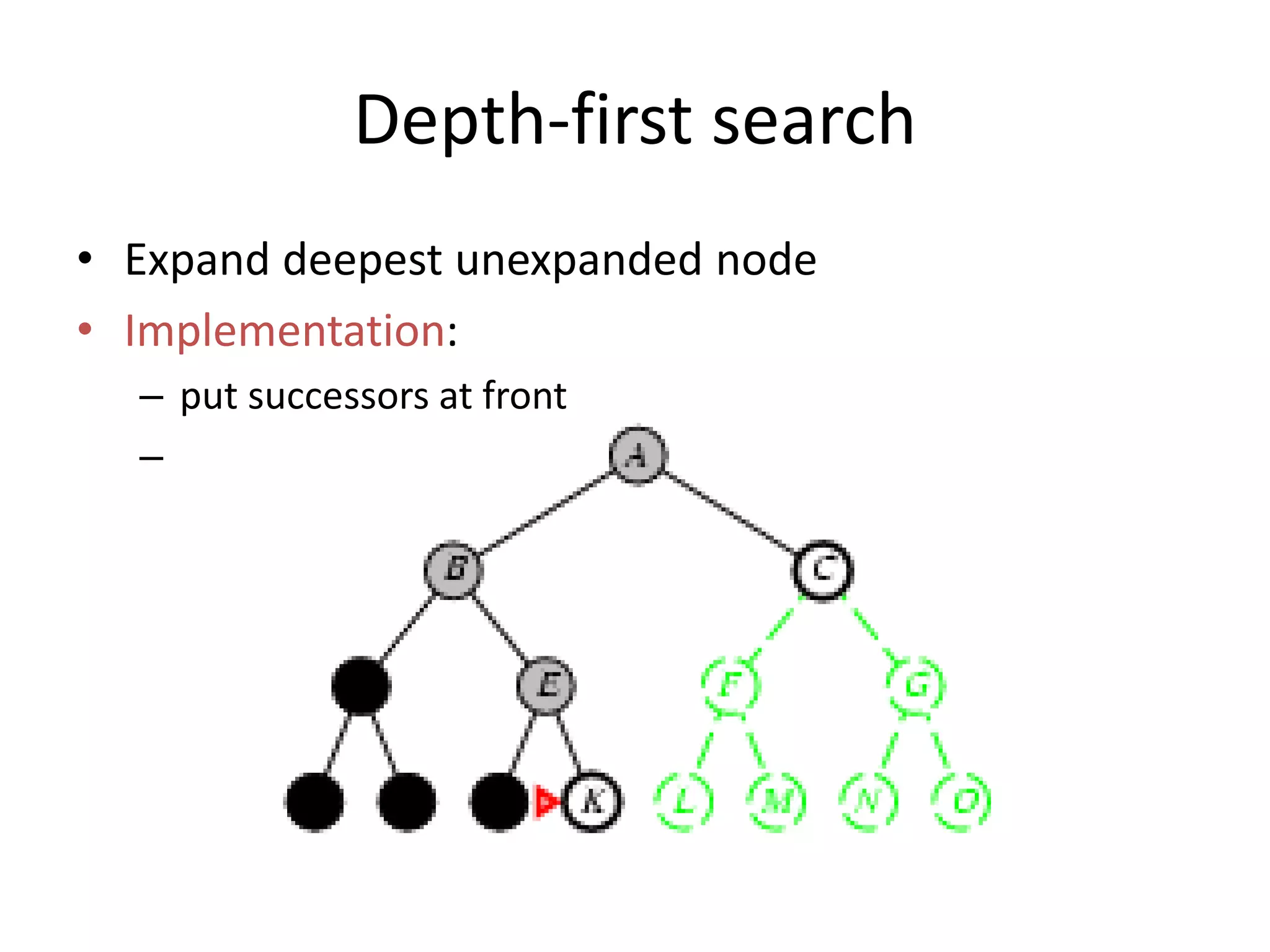
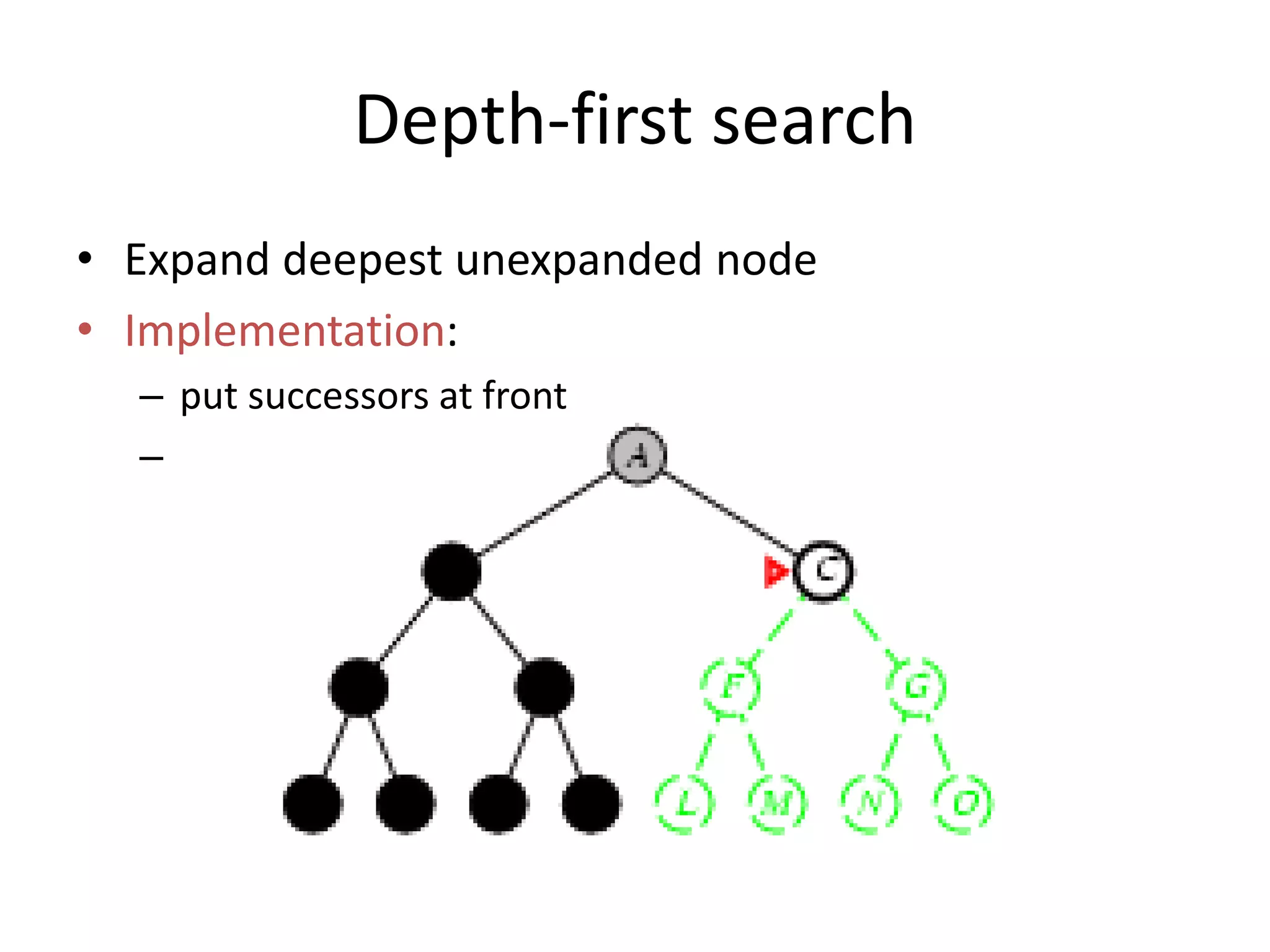
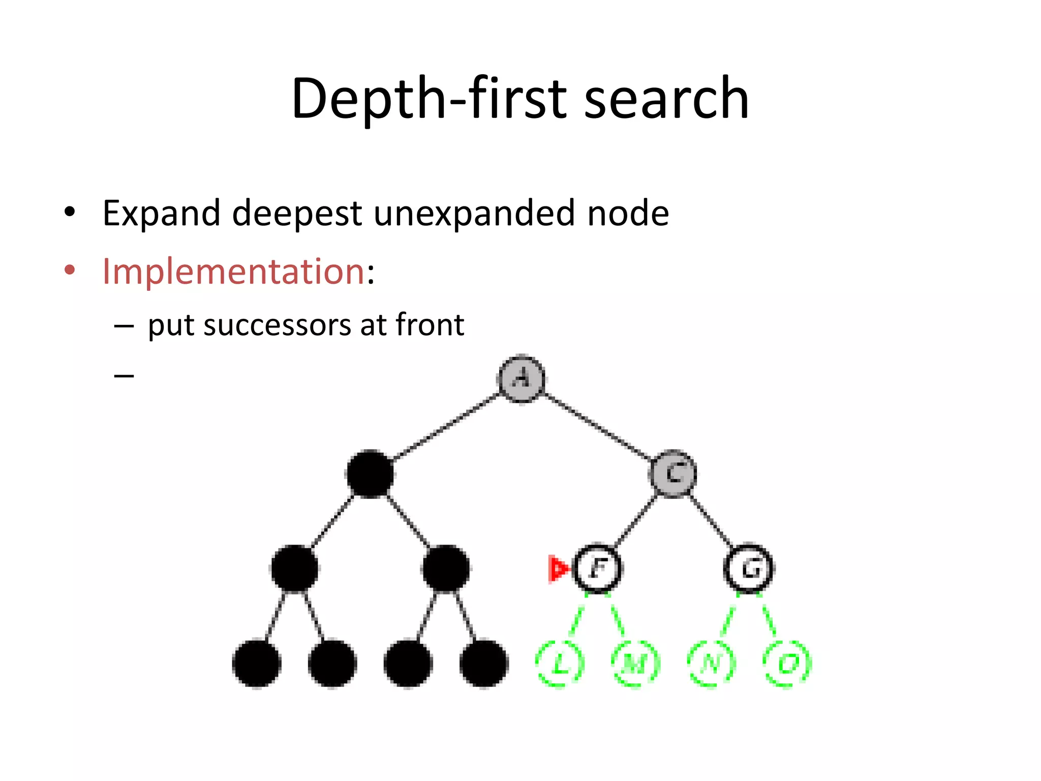
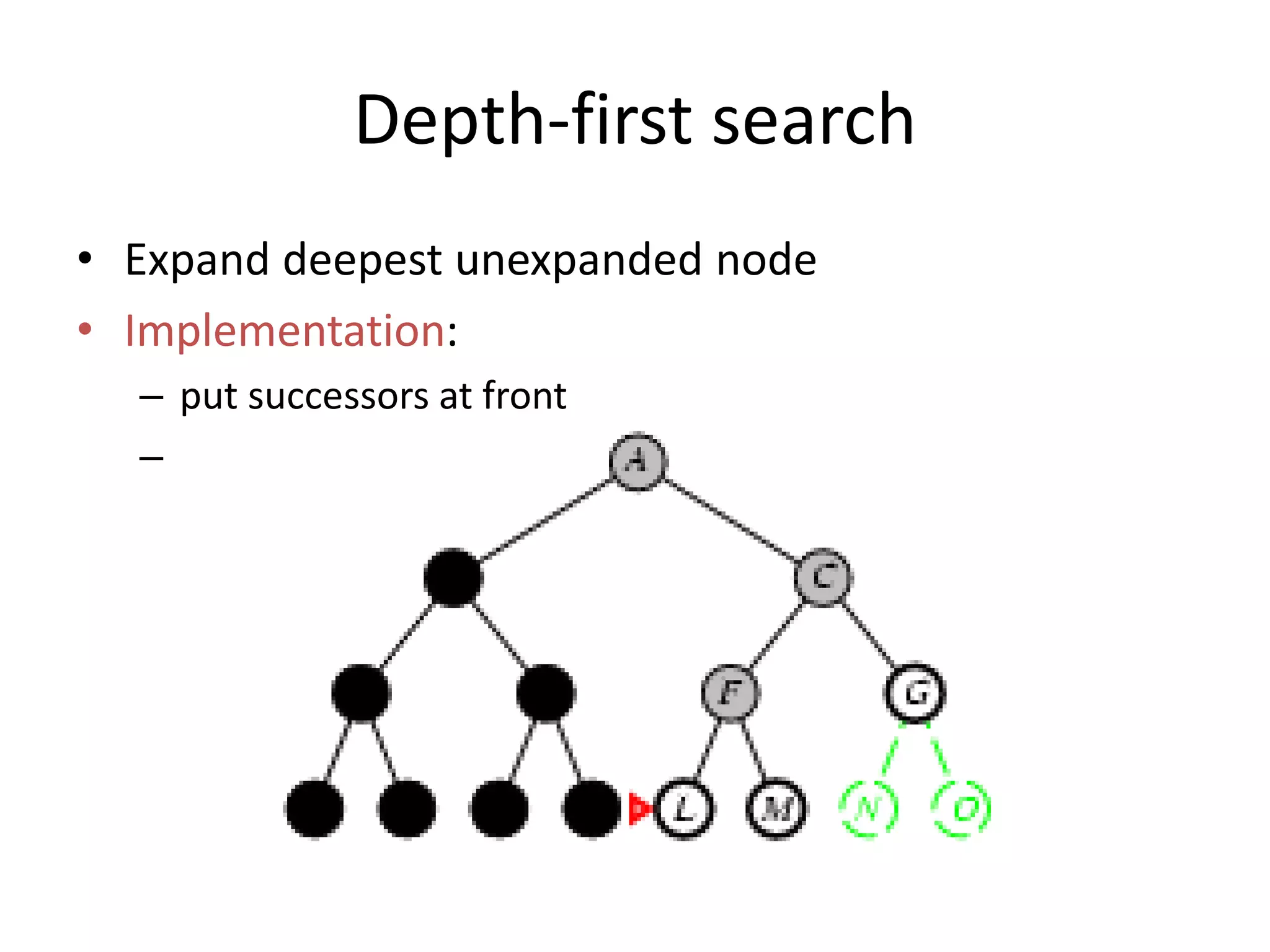
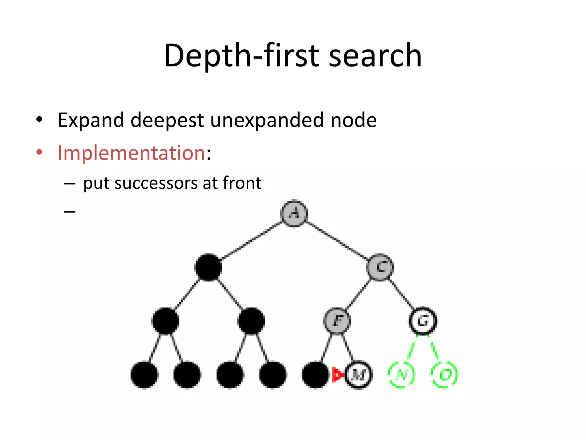
30. Depth-first search
Function depth ()
{
queue = []; // initialize an empty queue
state = root_node; // initialize the start state
while (true)
{
if is_goal (state)
then return SUCCESS
else add_to_front_of_queue (successors (state));
if queue == []
then report FAILURE;
state = queue [0]; // state = first item in queue
remove_first_item_from (queue);
}
}

32. Breadth-first search
• Expand shallowest unexpanded node
• Implementation:
– new successors go at end
–

33. Breadth-first search
• Expand shallowest unexpanded node
• Implementation:
– new successors go at end
–

34. Breadth-first search
• Expand shallowest unexpanded node
• Implementation:
– new successors go at end
–

35. Breadth-first search
• Expand shallowest unexpanded node
• Implementation:
– fringe is a FIFO queue, i.e., new successors go at
end
–

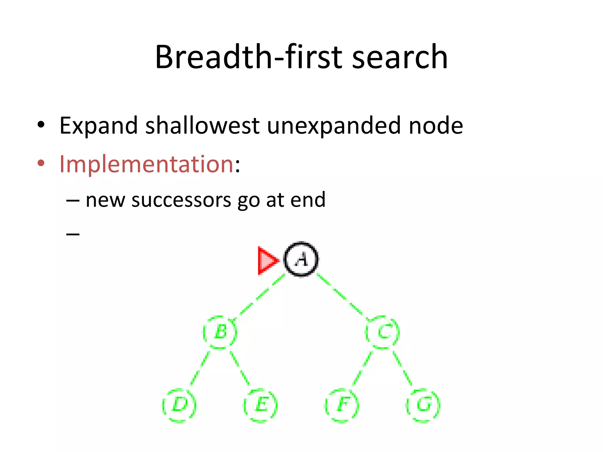
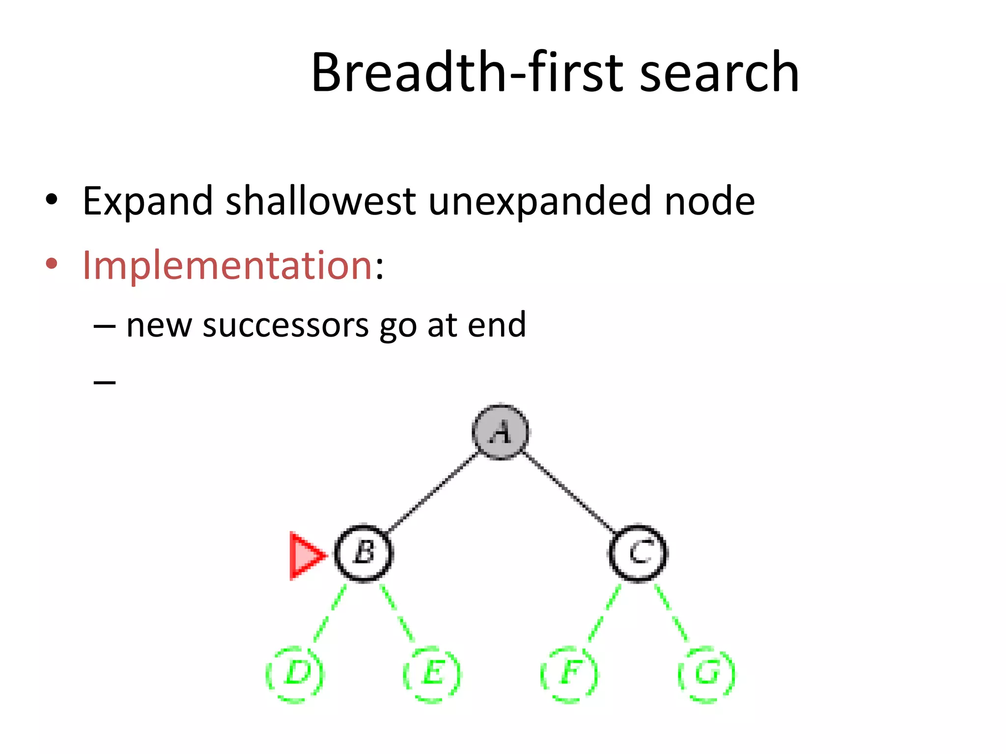
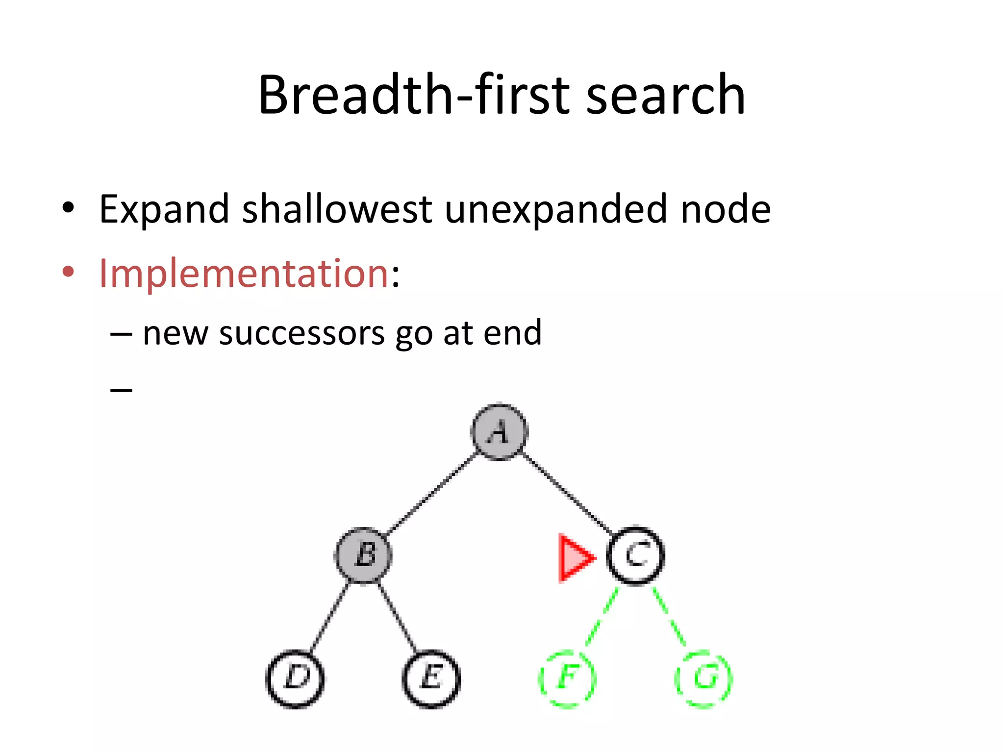
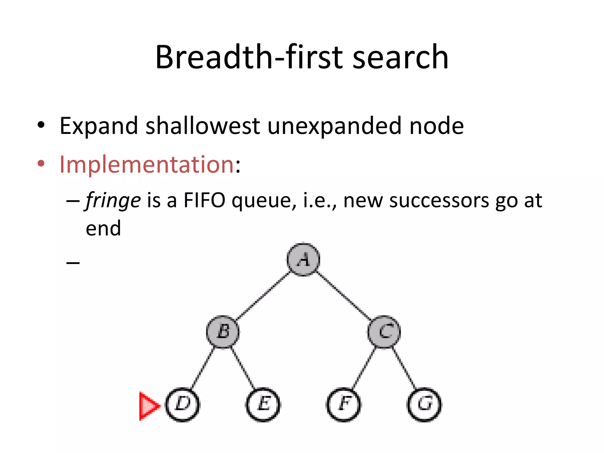
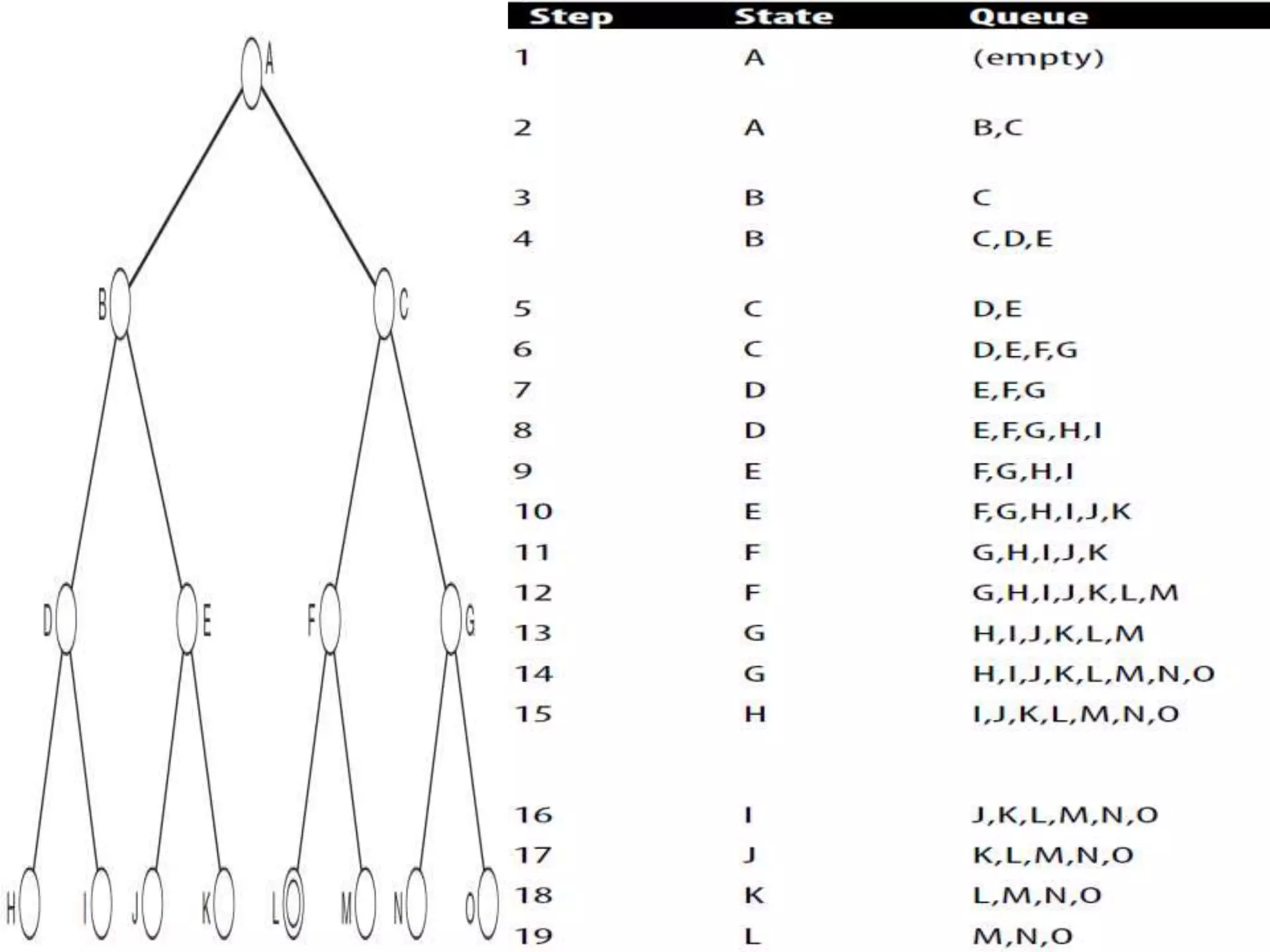
36. Breadth-first search
Function breadth ()
{
queue = []; // initialize an empty queue
state = root_node; // initialize the start state
while (true)
{
if is_goal (state)
then return SUCCESS
else add_to_back_of_queue (successors (state));
if queue == []
then report FAILURE;
state = queue [0]; // state = first item in queue
remove_first_item_from (queue);
}
}

38. Iterative deepening search l =0

39. Iterative deepening search l =1

40. Iterative deepening search l =2

41. Iterative deepening search l =3

42. Iterative deepening search
• Number of nodes generated in a depth-limited search to depth d with
branching factor b:
NDLS = b0 + b1 + b2 + … + bd-2 + bd-1 + bd
• GP
• Number of nodes generated in an iterative deepening search to depth d
with branching factor b:
NIDS = (d+1)b0 + d b^1 + (d-1)b^2 + … + 3bd-2 +2bd-1 + 1bd
• For b = 10, d = 5,
– NDLS = 1 + 10 + 100 + 1,000 + 10,000 + 100,000 = 111,111
–
– NIDS = 6 + 50 + 400 + 3,000 + 20,000 + 100,000 = 123,456
–
• Overhead = (123,456 - 111,111)/111,111 = 11%