This is the introduction to deep learning.

1. Deep Learning
Lecture 1 – Introduction to Deep Learning

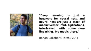
3. “Deep learning is just a
buzzword for neural nets, and
neural nets are just a stack of
matrix-vector mul- tiplications,
interleaved with some non-
linearities. No magic there.”
Ronan Collobert (Torch), 2011
3

4. Thies, Elgharib, Tewari, Theobalt and Niessner: Neural Voice Puppetry: Audio-driven Facial
Reenactment. ECCV, 2020. 4

5. Synthesia Demo,
2024
5

6. Deep Learning for Natural
Language

7. “Write a joke about deep neural networks that the students in my deep
learning class would find hilarious.”
OpenAI ChatGPT,
2024
7

8. Deep Learning for
Audio

9. Meta MusicGen,
2024
9

10. Google NotebookLM,
2024
10

11. Deep Learning for Images and
Video

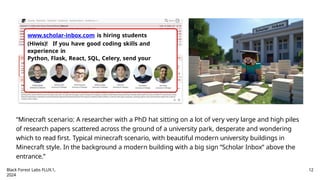
12. www.scholar-inbox.com is hiring students
(Hiwis)! If you have good coding skills and
experience in
Python, Flask, React, SQL, Celery, send your
application (CV+skills+transcripts) to:
a.geiger@uni-tuebingen.de
“Minecraft scenario: A researcher with a PhD hat sitting on a lot of very very large and high piles
of research papers scattered across the ground of a university park, desperate and wondering
which to read first. Typical minecraft scenario, with beautiful modern university buildings in
Minecraft style. In the background a modern building with a big sign ”Scholar Inbox” above the
entrance.”
Black Forest Labs FLUX.1,
2024
12

13. OpenAI SORA,
2024
13

14. Deep Learning for
3D

15. Chen, Xu, Esposito, Tang and Geiger: LaRa: Efficient Large-Baseline Radiance Fields. ECCV,
2024.
15

16. Gao, Liu, Chen, Geiger and Scho¨lkopf: GraphDreamer: Compositional 3D Scene Synthesis from Scene Graphs.
CVPR, 2024.
16

17. Deep Learning for Self-
Driving

18. Chitta, Prakash, Geiger: NEAT: Neural Attention Fields for End-to-End Autonomous Driving. ICCV,
2021.
18

19. Deep Learning for
Science

20. Google DeepMind AlphaFold – https://www.youtube.com/watch?v=gg7WjuFs8F4 20

21. Open Catalyst Project – https://www.youtube.com/playlist?list=PLU7acyFOb6DXgCTAi2TwKXaFD_i3C6hSL 21

22. Flipped
Classroom

23. Flipped Classroom
Regular Classroom
► Lecturer “reads” lecture in class
► Students digest content at
home
► Little “quality time”, no fun
Flipped Classroom
► Students watch lectures at
home
► Content discussed during
lecture 28

24. Flipped Classroom
Lecture
Videos
Lecture
Quiz
Exercise Helpdesk Exercise Quiz
1 Semester Week
Live Session
(Lecture and
Exercise)
Chat / Forum
Exercises
Study
Grou
p
24
https://uni-tuebingen.de/de/175884

25. Flipped
Classroom
25

26. History of Deep
Learning

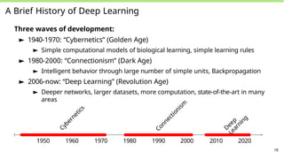
27. A Brief History of Deep Learning
Three waves of development:
► 1940-1970: “Cybernetics” (Golden Age)
► Simple computational models of biological learning, simple learning rules
► 1980-2000: “Connectionism” (Dark Age)
► Intelligent behavior through large number of simple units, Backpropagation
► 2006-now: “Deep Learning” (Revolution Age)
► Deeper networks, larger datasets, more computation, state-of-the-art in many
areas
1950 1960 1970 1980 1990 2000 2010 2020
C
y
b
e
r
n
e
t
i
c
s
C
o
n
n
e
c
t
i
o
n
i
s
m
D
e
e
p
L
e
a
r
n
i
n
g
18

28. A Brief History of Deep Learning
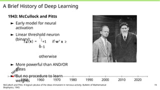
1943: McCullock and Pitts
► Early model for neural
activation
► Linear threshold neuron
(binary):
fw (x) =

+1 if wT x ≥
0
−1
otherwise
► More powerful than AND/OR
gates
► But no procedure to learn
weights
N
e
u
r
o
n
1950 1960 1970 1980 1990 2000 2010 2020
McCulloch and Pitts: A logical calculus of the ideas immanent in nervous activity. Bulletin of Mathematical
Biophysics, 1943.
19

29. A Brief History of Deep Learning
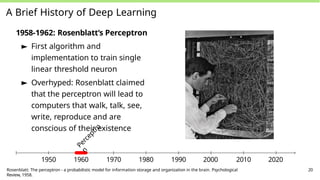
1958-1962: Rosenblatt’s Perceptron
► First algorithm and
implementation to train single
linear threshold neuron
► Optimization of perceptron
criterion:
Σ
T
L(w) = − w x y
n n
n M
∈
► Novikoff proved
convergence
P
e
r
c
e
p
t
r
o
n
1950 1960 1970 1980 1990 2000 2010 2020
Rosenblatt: The perceptron - a probabilistic model for information storage and organization in the brain. Psychological
Review, 1958.
20

30. A Brief History of Deep Learning
1958-1962: Rosenblatt’s Perceptron
► First algorithm and
implementation to train single
linear threshold neuron
► Overhyped: Rosenblatt claimed
that the perceptron will lead to
computers that walk, talk, see,
write, reproduce and are
conscious of their existence
P
e
r
c
e
p
t
r
o
n
1950 1960 1970 1980 1990 2000 2010 2020
Rosenblatt: The perceptron - a probabilistic model for information storage and organization in the brain. Psychological
Review, 1958.
20

31. A Brief History of Deep Learning
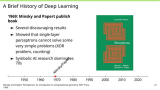
1969: Minsky and Papert publish
book
► Several discouraging results
► Showed that single-layer
perceptrons cannot solve some
very simple problems (XOR
problem, counting)
► Symbolic AI research dominates
70s
M
i
n
s
k
y
/
P
a
p
e
r
t
1950 1960 1970 1980 1990 2000 2010 2020
Minsky and Papert: Perceptrons: An introduction to computational geometry. MIT Press,
1969.
21

32. A Brief History of Deep Learning
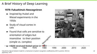
1979: Fukushima’s Neocognitron
► Inspired by Hubel and
Wiesel experiments in the
1950s
► Study of visual cortex in
cats
► Found that cells are sensitive to
orientation of edges but
insensitive to their position
(simple vs. complex)
► H&W received Nobel prize in 1981
N
e
o
c
o
g
n
i
t
r
o
n
1950 1960 1970 1980 1990 2000 2010 2020
Fukushima: Neural network model for a mechanism of pattern recognition unaffected by shift in position. IECE (in
Japanese), 1979.
22

33. A Brief History of Deep Learning
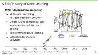
1979: Fukushima’s Neocognitron
► Multi-layer processing
to create intelligent behavior
► Simple (S) and complex (C) cells
implement convolution and
pooling
► Reinforcement based learning
► Inspiration for modern
ConvNets
N
e
o
c
o
g
n
i
t
r
o
n
1950 1960 1970 1980 1990 2000 2010 2020
Fukushima: Neural network model for a mechanism of pattern recognition unaffected by shift in position. IECE (in
Japanese), 1979.
22

34. A Brief History of Deep Learning
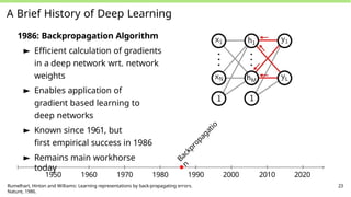
1986: Backpropagation Algorithm
► Efficient calculation of gradients
in a deep network wrt. network
weights
► Enables application of
gradient based learning to
deep networks
► Known since 1961, but
first empirical success in 1986
► Remains main workhorse
today
B
a
c
k
p
r
o
p
a
g
a
t
i
o
n
1950 1960 1970 1980 1990 2000 2010 2020
Rumelhart, Hinton and Williams: Learning representations by back-propagating errors.
Nature, 1986.
23

35. A Brief History of Deep Learning
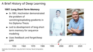
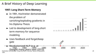
1997: Long Short-Term Memory
► In 1991, Hochreiter demonstrated
the problem of
vanishing/exploding gradients in
his Diploma Thesis
► Led to development of long-short
term memory for sequence
modeling
► Uses feedback and forget/keep
gate
L
S
T
M
1950 1960 1970 1980 1990 2000 2010 2020
Hochreiter, Schmidhuber: Long short-term memory. Neural Computation,
1997.
24

36. A Brief History of Deep Learning
1997: Long Short-Term Memory
► In 1991, Hochreiter demonstrated
the problem of
vanishing/exploding gradients in
his Diploma Thesis
► Led to development of long-short
term memory for sequence
modeling
► Uses feedback and forget/keep
gate
► Revolutionized NLP (e.g. at
Google) many years later (2015)
L
S
T
M
1950 1960 1970 1980 1990 2000 2010 2020
Hochreiter, Schmidhuber: Long short-term memory. Neural Computation,
1997.
24

37. A Brief History of Deep Learning
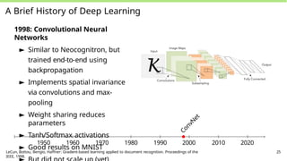
1998: Convolutional Neural
Networks
► Similar to Neocognitron, but
trained end-to-end using
backpropagation
► Implements spatial invariance
via convolutions and max-
pooling
► Weight sharing reduces
parameters
► Tanh/Softmax activations
► Good results on MNIST
C
o
n
v
N
e
t
1950 1960 1970 1980 1990 2000 2010 2020
LeCun, Bottou, Bengio, Haffner: Gradient-based learning applied to document recognition. Proceedings of the
IEEE, 1998.
25

38. A Brief History of Deep Learning
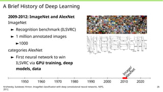
2009-2012: ImageNet and AlexNet
ImageNet
► Recognition benchmark (ILSVRC)
► 1 million annotated images
►1000
categories AlexNet
► First neural network to win
ILSVRC via GPU training, deep
models, data
I
m
a
g
e
/
A
l
e
x
N
e
t
1950 1960 1970 1980 1990 2000 2010 2020
Krizhevsky, Sutskever, Hinton. ImageNet classification with deep convolutional neural networks. NIPS,
2012.
26

39. A Brief History of Deep Learning
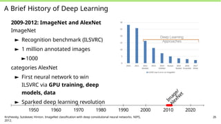
2009-2012: ImageNet and AlexNet
ImageNet
► Recognition benchmark (ILSVRC)
► 1 million annotated images
►1000
categories AlexNet
► First neural network to win
ILSVRC via GPU training, deep
models, data
► Sparked deep learning revolution
I
m
a
g
e
/
A
l
e
x
N
e
t
1950 1960 1970 1980 1990 2000 2010 2020
Krizhevsky, Sutskever, Hinton. ImageNet classification with deep convolutional neural networks. NIPS,
2012.
26

40. A Brief History of Deep Learning
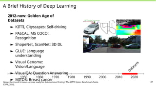
2012-now: Golden Age of
Datasets
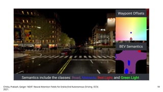
► KITTI, Cityscapes: Self-driving
► PASCAL, MS COCO:
Recognition
► ShapeNet, ScanNet: 3D DL
► GLUE: Language
understanding
► Visual Genome:
Vision/Language
► VisualQA: Question Answering
► MITOS: Breast cancer
D
a
t
a
s
e
t
s
1950 1960 1970 1980 1990 2000 2010 2020
Geiger, Lenz and Urtasun. Are we ready for Autonomous Driving? The KITTI Vision Benchmark Suite.
CVPR, 2012.
27

41. A Brief History of Deep Learning
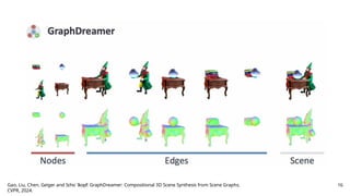
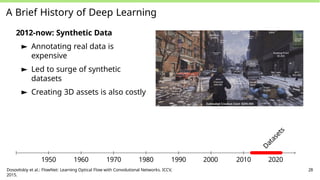
2012-now: Synthetic Data
► Annotating real data is
expensive
► Led to surge of synthetic
datasets
► Creating 3D assets is also costly
D
a
t
a
s
e
t
s
1950 1960 1970 1980 1990 2000 2010 2020
Dosovitskiy et al.: FlowNet: Learning Optical Flow with Convolutional Networks. ICCV,
2015.
28

42. A Brief History of Deep Learning
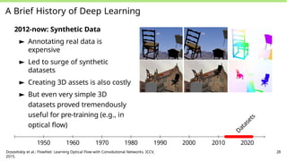
2012-now: Synthetic Data
► Annotating real data is
expensive
► Led to surge of synthetic
datasets
► Creating 3D assets is also costly
► But even very simple 3D
datasets proved tremendously
useful for pre-training (e.g., in
optical flow)
D
a
t
a
s
e
t
s
1950 1960 1970 1980 1990 2000 2010 2020
Dosovitskiy et al.: FlowNet: Learning Optical Flow with Convolutional Networks. ICCV,
2015.
28

43. A Brief History of Deep Learning
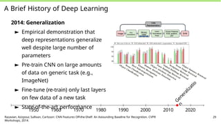
2014: Generalization
► Empirical demonstration that
deep representations generalize
well despite large number of
parameters
► Pre-train CNN on large amounts
of data on generic task (e.g.,
ImageNet)
► Fine-tune (re-train) only last layers
on few data of a new task
► State-of-the-art performance
G
e
n
e
r
a
l
i
z
a
t
i
o
n
1950 1960 1970 1980 1990 2000 2010 2020
Razavian, Azizpour, Sullivan, Carlsson: CNN Features Off-the-Shelf: An Astounding Baseline for Recognition. CVPR
Workshops, 2014.
29

44. A Brief History of Deep Learning
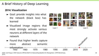
2014: Visualization
► Goal: provide insights into what
the network (black box) has
learned
► Visualized image regions that
most strongly activate various
neurons at different layers of the
network
► Found that higher levels capture
more abstract semantic
information
V
i
s
u
a
l
i
z
a
t
i
o
n
1950 1960 1970 1980 1990 2000 2010 2020
Zeiler and Fergus: CNN Features Off-the-Shelf: An Astounding Baseline for Recognition. CVPR Workshops,
2014.
30

45. A Brief History of Deep Learning
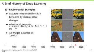
2014: Adversarial Examples
► Accurate image classifiers can
be fooled by imperceptible
changes
► Adversarial example:
∆ x
2
x+argmin {∆x : f ( x+ ∆ x ) /= f
(x)
}
► All images classified as
“ostrich”
1950 1960 1970 1980 1990 2000 2010 2020
Szegedy et al.: Intriguing properties of neural networks. ICLR,
2014.
31

46. A Brief History of Deep
Learning
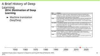
2014: Domination of Deep
Learning
► Machine translation
(Seq2Seq)
1950 1960 1970 1980 1990 2000 2010 2020
Sutskever, Vinyals, Quoc: Sequence to Sequence Learning with Neural Networks. NIPS,
2014.
32

47. A Brief History of Deep Learning
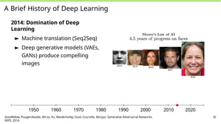
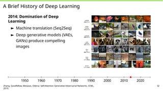
2014: Domination of Deep
Learning
► Machine translation (Seq2Seq)
► Deep generative models (VAEs,
GANs) produce compelling
images
1950 1960 1970 1980 1990 2000 2010 2020
Goodfellow, Pouget-Abadie, Mirza, Xu, Warde-Farley, Ozair, Courville, Bengio: Generative Adversarial Networks.
NIPS, 2014.
32

48. A Brief History of Deep Learning
2014: Domination of Deep
Learning
► Machine translation (Seq2Seq)
► Deep generative models (VAEs,
GANs) produce compelling
images
1950 1960 1970 1980 1990 2000 2010 2020
Zhang, Goodfellow, Metaxas, Odena: Self-Attention Generative Adversarial Networks. ICML,
2019.
32

49. A Brief History of Deep Learning
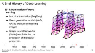
2014: Domination of Deep
Learning
► Machine translation (Seq2Seq)
► Deep generative models (VAEs,
GANs) produce compelling
images
► Graph Neural Networks
(GNNs) revolutionize the
prediction of molecular
properties
1950 1960 1970 1980 1990 2000 2010 2020
Duvenaud et al.: Convolutional Networks on Graphs for Learning Molecular Fingerprints.
NIPS 2015.
32

50. A Brief History of Deep Learning
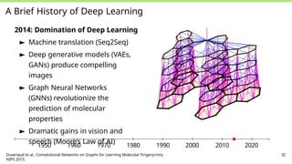
2014: Domination of Deep Learning
► Machine translation (Seq2Seq)
► Deep generative models (VAEs,
GANs) produce compelling
images
► Graph Neural Networks
(GNNs) revolutionize the
prediction of molecular
properties
► Dramatic gains in vision and
speech (Moore’s Law of AI)
1950 1960 1970 1980 1990 2000 2010 2020
Duvenaud et al.: Convolutional Networks on Graphs for Learning Molecular Fingerprints.
NIPS 2015.
32

51. A Brief History of Deep Learning
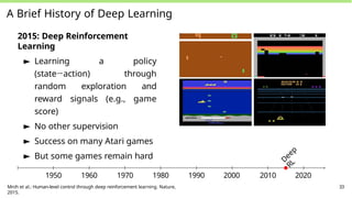
2015: Deep Reinforcement
Learning
► Learning a policy
(state→action) through
random exploration and
reward signals (e.g., game
score)
► No other supervision
► Success on many Atari games
► But some games remain hard
D
e
e
p
R
L
1950 1960 1970 1980 1990 2000 2010 2020
Mnih et al.: Human-level control through deep reinforcement learning. Nature,
2015.
33

52. A Brief History of Deep Learning
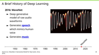
2016: WaveNet
► Deep generative
model of raw audio
waveforms
► Generates speech
which mimics human
voice
► Generates music
W
a
v
e
N
e
t
1950 1960 1970 1980 1990 2000 2010 2020
Oord et al.: WaveNet: A Generative Model for Raw Audio. Arxiv,
2016.
34

53. A Brief History of Deep Learning
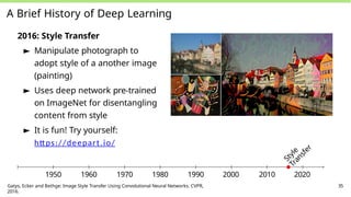
2016: Style Transfer
► Manipulate photograph to
adopt style of a another image
(painting)
► Uses deep network pre-trained
on ImageNet for disentangling
content from style
► It is fun! Try yourself:
https://deepart.io/
S
t
y
l
e
T
r
a
n
s
f
e
r
1950 1960 1970 1980 1990 2000 2010 2020
Gatys, Ecker and Bethge: Image Style Transfer Using Convolutional Neural Networks. CVPR,
2016.
35

54. A Brief History of Deep Learning
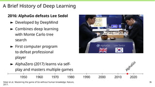
2016: AlphaGo defeats Lee Sedol
► Developed by DeepMind
► Combines deep learning
with Monte Carlo tree
search
► First computer program
to defeat professional
player
► AlphaZero (2017) learns via self-
play and masters multiple games
A
l
p
h
a
G
o
1950 1960 1970 1980 1990 2000 2010 2020
Silver et al.: Mastering the game of Go without human knowledge. Nature,
2017.
36

55. A Brief History of Deep Learning
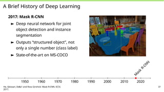
2017: Mask R-CNN
► Deep neural network for joint
object detection and instance
segmentation
► Outputs “structured object”, not
only a single number (class label)
► State-of-the-art on MS-COCO
M
a
s
k
R
-
C
N
N
1950 1960 1970 1980 1990 2000 2010 2020
He, Gkioxari, Dolla´r and Ross Girshick: Mask R-CNN. ICCV,
2017.
37

56. A Brief History of Deep
Learning
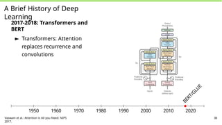
2017-2018: Transformers and
BERT
► Transformers: Attention
replaces recurrence and
convolutions
B
E
R
T
/
G
L
U
E
1950 1960 1970 1980 1990 2000 2010 2020
Vaswani et al.: Attention is All you Need. NIPS
2017.
38

57. A Brief History of Deep Learning
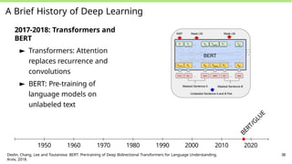
2017-2018: Transformers and
BERT
► Transformers: Attention
replaces recurrence and
convolutions
► BERT: Pre-training of
language models on
unlabeled text
B
E
R
T
/
G
L
U
E
1950 1960 1970 1980 1990 2000 2010 2020
Devlin, Chang, Lee and Toutanova: BERT: Pre-training of Deep Bidirectional Transformers for Language Understanding.
Arxiv, 2018.
38

58. A Brief History of Deep Learning
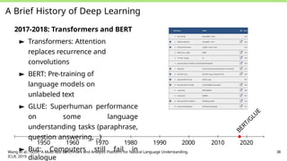
2017-2018: Transformers and BERT
► Transformers: Attention
replaces recurrence and
convolutions
► BERT: Pre-training of
language models on
unlabeled text
► GLUE: Superhuman performance
on some language
understanding tasks (paraphrase,
question answering, ..)
► But: Computers still fail in
dialogue
B
E
R
T
/
G
L
U
E
1950 1960 1970 1980 1990 2000 2010 2020
Wang et al.: GLUE: A Multi-Task Benchmark and Analysis Platform for Natural Language Understanding.
ICLR, 2019.
38

59. A Brief History of Deep Learning
2017-2018: Transformers and BERT
► Transformers: Attention
replaces recurrence and
convolutions
► BERT: Pre-training of
language models on
unlabeled text
► GLUE: Superhuman performance
on some language
understanding tasks (paraphrase,
question answering, ..)
► But: Computers still fail in
dialogue
B
E
R
T
/
G
L
U
E
1950 1960 1970 1980 1990 2000 2010 2020
Wang et al.: GLUE: A Multi-Task Benchmark and Analysis Platform for Natural Language Understanding.
ICLR, 2019.
38

60. A Brief History of Deep Learning
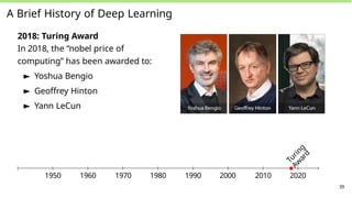
2018: Turing Award
In 2018, the “nobel price of
computing” has been awarded to:
► Yoshua Bengio
► Geoffrey Hinton
► Yann LeCun
T
u
r
i
n
g
A
w
a
r
d
1950 1960 1970 1980 1990 2000 2010 2020
39

61. A Brief History of Deep Learning
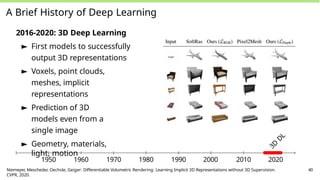
2016-2020: 3D Deep Learning
► First models to successfully
output 3D representations
► Voxels, point clouds,
meshes, implicit
representations
► Prediction of 3D
models even from a
single image
► Geometry, materials,
light, motion
3
D
D
L
1950 1960 1970 1980 1990 2000 2010 2020
Niemeyer, Mescheder, Oechsle, Geiger: Differentiable Volumetric Rendering: Learning Implicit 3D Representations without 3D Supervision.
CVPR, 2020.
40

62. A Brief History of Deep Learning
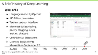
2020: GPT-3
► Language model by OpenAI
► 175 Billion parameters
► Text-in / text-out interface
► Many use cases: coding,
poetry, blogging, news
articles, chatbots
► Controversial discussions
► Licensed exclusively to
Microsoft on September 22,
2020
G
P
T
-
3
1950 1960 1970 1980 1990 2000 2010 2020
Brown et al.: Language Models are Few-Shot Learners. Arxiv,
2020.
41

63. A Brief History of Deep Learning
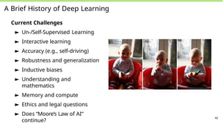
Current Challenges
► Un-/Self-Supervised Learning
► Interactive learning
► Accuracy (e.g., self-driving)
► Robustness and generalization
► Inductive biases
► Understanding and
mathematics
► Memory and compute
► Ethics and legal questions
► Does “Moore’s Law of AI”
continue?
42

64. Machine Learning
Basics

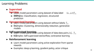
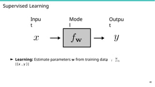
65. Learning Problems
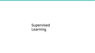
45
► Supervised
learning
► Learn model parameters using dataset of data-label
pairs {
i i
(x , y )}N
i = 1
► Examples: Classification, regression, structured
prediction
► Unsupervised learning
i
► Learn model parameters using dataset without labels
{x }
N
i = 1
► Examples: Clustering, dimensionality reduction, generative
models
► Self-supervised learning
i
► Learn model parameters using dataset of data-data pairs {(x ,
x )}
′ N
i i = 1
► Examples: Self-supervised stereo/flow, contrastive learning
► Reinforcement learning
► Learn model parameters using active exploration from sparse
rewards
► Examples: deep q learning, gradient policy, actor critique

66. Supervised
Learning

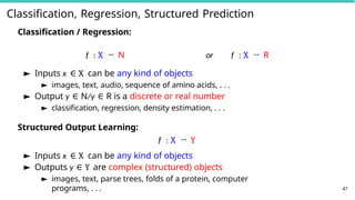
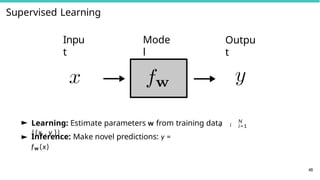
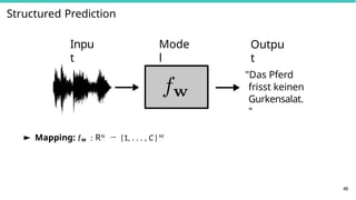
67. Classification, Regression, Structured Prediction
47
Classification / Regression:
f : X → N or f : X → R
► Inputs x ∈ X can be any kind of objects
► images, text, audio, sequence of amino acids, . . .
► Output y ∈ N/y ∈ R is a discrete or real number
► classification, regression, density estimation, . . .
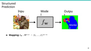
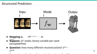
Structured Output Learning:
f : X → Y
► Inputs x ∈ X can be any kind of objects
► Outputs y ∈ Y are complex (structured) objects
► images, text, parse trees, folds of a protein, computer
programs, . . .

68. Supervised
Learning
Inpu
t
Outpu
t
Mode
l
48

69. Supervised Learning
Inpu
t
Outpu
t
Mode
l
►
48
i i
Learning: Estimate parameters w from training data
{(x , y )}
N
i=1

70. Supervised Learning
Inpu
t
Outpu
t
Mode
l
►
48
i i
Learning: Estimate parameters w from training data
{(x , y )}
N
i=1
► Inference: Make novel predictions: y =
fw (x)

71. Classification
Inpu
t
"Beach
"
Mode
l
Outpu
t
48
► Mapping: fw : RW × H → {“Beach”, “No
Beach”}

72. Regressio
n
Inpu
t
143,52 €
Mode
l
Outpu
t
► Mapping: fw : RN → R
48

73. Structured Prediction
Inpu
t
"Das Pferd
frisst keinen
Gurkensalat.
"
Mode
l
Outpu
t
► Mapping: fw : RN → {1, . . . , C}M
48

74. Structured
Prediction
Inpu
t
Mode
l
Can
Monke
y
48
Outpu
t
► Mapping: fw : RW × H → {1, . . . , C}W × H

75. Structured Prediction
Inpu
t
Mode
l
Outpu
t
w
48
► Mapping: f : RW × H × N → {0,
1}M 3
► Suppose: 323 voxels, binary variable per voxel
(occupied/free)
► Question: How many different reconstructions? 2323
=
232768

76. Linear
Regression

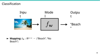
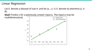
77. Linear Regression
Let X denote a dataset of size N and let (xi , yi ) ∈ X denote its elements (yi ∈
R).
Goal: Predict y for a previously unseen input x. The input x may be
multidimensional.
1.0
0.5
0.0
0.5
1.0
1.5
1.00 0.75 0.50 0.25 0.00 0.25 0.50 0.75 1.00
x
1.5
50
y
Ground Truth
Noisy Observations

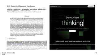
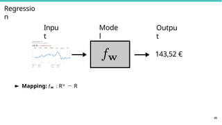
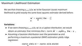
78. Linear Regression
The error function E(w) measures the displacement along the y dimension
between the data points (green) and the model f (x, w) (red) specified by the
parameters w.
f (x, w) = wT
x
N
Σ
i
E(w) = (f (x ,
w) i=1
N
i
—
y )
2
Σ
i=1
T
i
= x w − yi
2
= X w − y
2
2
1.5
1.00 0.75 0.50 0.25 0.00 0.25 0.50 0.75 1.00
x
1.0
0.5
0.0
0.5
1.0
1.5
y
Ground Truth
Noisy Observations
Linear Fit
Here: x = [1, x]T ⇒ f (x, w) = w0 +
w1x
51

79. Linear Regression
2
52
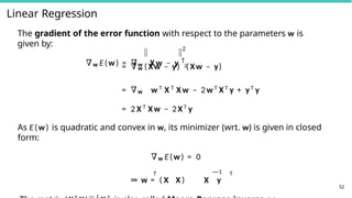
The gradient of the error function with respect to the parameters w is
given by:
∇w E(w) = ∇w X w − y 2
T
= ∇w ( Xw − y) ( Xw − y)
= ∇w w T
X T
X w − 2w T
X T
y + yT
y
= 2 X T
Xw − 2XT
y
As E(w) is quadratic and convex in w, its minimizer (wrt. w) is given in closed
form:
∇w E(w) = 0
T —1 T
⇒ w = ( X X ) X y

80. Example: Line
Fitting

81. Line Fitting
1.5
1.0
0.5
0.0
0.5
1.0
1.5
y
Ground Truth
Noisy Observations
Linear Fit
1.00 0.75 0.50 0.25 0.00 0.25 0.50 0.75 1.00 1.0 0.5 0.0
x
0.5 1.0 1.5 2.0
w1
0
54
1
2
3
4
5
6
7
8
Error
Error Curve
Minimum
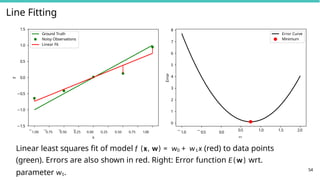
Linear least squares fit of model f (x, w) = w0 + w1x (red) to data points
(green). Errors are also shown in red. Right: Error function E(w) wrt.
parameter w1.

82. Example: Polynomial Curve
Fitting

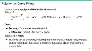
83. Polynomial Curve Fitting
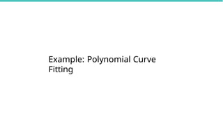
56
Let us choose a polynomial of order M to model
dataset X:
M
Σ
f (x, w) =
w
j xj
= wT
x with features x = (1, x1
, x2
, . . . , xM
)T
j = 0
Tasks:
► Training: Estimate w from dataset X
►Inference: Predict y for novel x given
estimated w Note:
► Features can be anything, including multi-dimensional inputs (e.g., images,
audio), radial basis functions, sine/cosine functions, etc. In this example:
monomials.

84. Polynomial Curve Fitting
57
Let us choose a polynomial of order M to model the
dataset X:
M
Σ
f (x, w) =
w
j
j T
x = w x
j = 0
How can we estimate w from
X?
with
features
x = (1, x1
, x2
, . . . , xM
)T

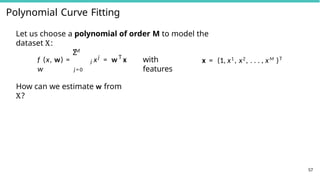
85. Polynomial Curve Fitting
The error function from above is quadratic in w but
not in x:
E(w) =
N
Σ 2
(f (xi , w) − yi ) =
N
Σ
T
2
w xi − yi =


N M
Σ Σ
j
j
i
w x − yi
2

i=1 i=1 i=1 j = 0
It can be rewritten in the matrix-vector notation (i.e., as linear regression
problem)
E(w) = X w − y
2
2
58
with feature matrix X , observation vector y and weight
vector w:
X = 
. .
.
. . .
.
1 xi
 x2
i . . . x
.
M
i
. .
.
. .
.
.
.
 

 y =
.
.
yi
.
.
 
 
  w =



w0
.
.
wM




86. Polynomial Curve Fitting
Results

87. Polynomial Curve Fitting
1.0
0.5
0.0
0.5
1.0
1.5
y
M = 0 Ground Truth
Noisy Observations
Polynomial Fit
Test Set
0.0 0.2 0.4 0.6 0.8 1.0 0.0 0.2 0.4 0.6 0.8 1.0
1.5 1.5
1.0
0.5
0.0
0.5
1.0
1.5
y
M = 1 Ground Truth
Noisy Observations
Polynomial Fit
Test Set
60
x
x
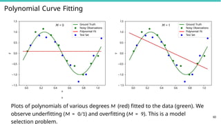
Plots of polynomials of various degrees M (red) fitted to the data (green). We
observe underfitting (M = 0/1) and overfitting (M = 9). This is a model
selection problem.

88. Polynomial Curve Fitting
1.0
0.5
0.0
0.5
1.0
1.5
y
M = 3 Ground Truth
Noisy Observations
Polynomial Fit
Test Set
1.0
0.5
0.0
0.5
1.0
1.5
y
M = 9 Ground Truth
Noisy Observations
Polynomial Fit
Test Set
1.5 1.5
0.0 0.2 0.4 0.6
x
0.8 1.0 0.0 0.2 0.4 0.6
x
0.8 1.0
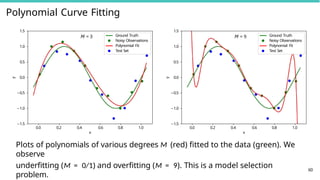
Plots of polynomials of various degrees M (red) fitted to the data (green). We
observe
underfitting (M = 0/1) and overfitting (M = 9). This is a model selection
problem.
60

89. Capacity, Overfitting and Underfitting
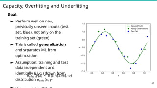
Goal:
► Perform well on new,
previously unseen inputs (test
set, blue), not only on the
training set (green)
► This is called generalization
and separates ML from
optimization
► Assumption: training and test
data independent and
identically (i.i.d.) drawn from
distribution pdata(x, y)
0.0 0.2 0.4 0.6 0.8 1.0
1.5
1.0
0.5
0.0
0.5
1.0
1.5
y
Ground Truth
Noisy Observations
Test Set
pdata(y|x) = N(sin(2πx), σ) x
61

90. Capacity, Overfitting and Underfitting
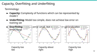
Terminology:
► Capacity: Complexity of functions which can be represented by
model f
► Underfitting: Model too simple, does not achieve low error on
training set
► Overfitting: Training error small, but test error (= generalization
error) large
0.0 0.2 0.8 1.0
0.4 0.6
x
1.5
1.0
0.5
0.0
0.5
1.0
1.5
y
M =1 Ground Truth
Noisy Observations
Polynomial Fit
Test Set
0.0 0.2 0.8 1.0
0.4 0.6
x
1.5
1.0
0.5
0.0
0.5
1.0
1.5
y
M =3 Ground Truth
Noisy Observations
Polynomial Fit
Test Set
0.0 0.2 0.8 1.0
0.4 0.6
x
1.5
1.0
0.5
0.0
0.5
1.0
1.5
y
M =9
Capacity too
low
Capacity about
right
Capacity too
high 62
Ground Truth
Noisy Observations
Polynomial Fit
Test Set

91. Capacity, Overfitting and Underfitting
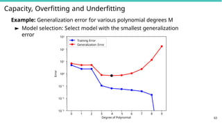
Example: Generalization error for various polynomial degrees M
► Model selection: Select model with the smallest generalization
error
0 1 2 3 4 5 6 7 8 9
Degree of Polynomial
10 3
10 2
10 1
100
101
103
Training Error
Generalization Error
102
Error
63

92. Capacity, Overfitting and Underfitting
Training
64
60%
Validation
20%
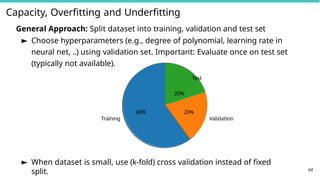
General Approach: Split dataset into training, validation and test set
► Choose hyperparameters (e.g., degree of polynomial, learning rate in
neural net, ..) using validation set. Important: Evaluate once on test set
(typically not available).
Test
20%
► When dataset is small, use (k-fold) cross validation instead of fixed
split.

93. Ridge
Regression

94. Ridge Regression
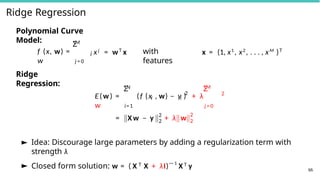
Polynomial Curve
Model: M
Σ
f (x, w) =
w
j xj
= wT
x
j = 0
Ridge
Regression:
with
features
x = (1, x1
, x2
, . . . , xM
)T
N
Σ
i i
2
M
Σ
i=1 j = 0
E(w) = (f (x , w) − y ) + λ
w
2
2
2
= X w − y + λ w
2
2
66
► Idea: Discourage large parameters by adding a regularization term with
strength λ
► Closed form solution: w = ( X T X + λI)—1
X T y

95. Ridge Regression
0.0 0.2
1.5
1.0
0.5
0.0
0.5
1.0
1.5
y
M = 9, = 10 8 Ground Truth
Noisy Observations
Polynomial Fit
Test Set
0.4 0.6 0.8 1.0 0.0 0.2
x
0.4 0.6 0.8 1.0
x
1.5
1.0
0.5
0.0
0.5
1.0
1.5
y
M = 9, = 103 Ground Truth
Noisy Observations
Polynomial Fit
Test Set
67
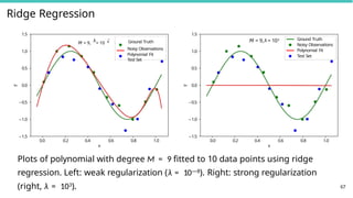
Plots of polynomial with degree M = 9 fitted to 10 data points using ridge
regression. Left: weak regularization (λ = 10—8). Right: strong regularization
(right, λ = 103).

96. Ridge Regression
10 13 10 12 10 11 10 10 10 9
10 8
10 7
10 6
Regularization Weight
100000
50000
0
50000
100000
Model Weights
10 11
10 8 5
10 10 2 101
104
Regularization weight
10 2
10 1
100
101
102
Error
68
Training Error
Generalization Error
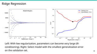
Left: With low regularization, parameters can become very large (ill-
conditioning). Right: Select model with the smallest generalization error
on the validation set.

97. Estimators, Bias and
Variance

98. Estimators, Bias and Variance
70
Point Estimator:
► A point estimator g(·) is function that maps a dataset X to model
parameters wˆ :
wˆ = g(X)
► Example: Estimator of ridge regression model: wˆ = ( X T X + λI)—1
XT y
► We use the hat notation to denote that wˆ is an estimate
► A good estimator is a function that returns a parameter set close to the
true one
► The data X = {(xi , yi )} is drawn from a random process (xi , yi ) ∼ pdata(·)
► Thus, any function of the data is random and wˆ is a random variable.

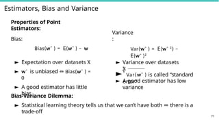
99. Estimators, Bias and Variance
Properties of Point
Estimators:
Bias:
Bias(wˆ ) = E(wˆ ) − w
► Expectation over datasets X
► wˆ is unbiased ⇔ Bias(wˆ ) =
0
► A good estimator has little
bias
Variance
:
Var(wˆ ) = E(wˆ 2
) −
E(wˆ )2
► Variance over datasets
X
►√
Var(wˆ ) is called “standard
error”
71
► A good estimator has low
variance
Bias-Variance Dilemma:
► Statistical learning theory tells us that we can’t have both ⇒ there is a
trade-off

100. Estimators, Bias and Variance
0.0 0.2 0.8 1.0
0.4 0.6
x
0.8
0.6
0.4
0.2
0.0
0.2
0.4
0.6
0.8
y
= 10 8
Estimates
Ground Truth
Mean
0.0 0.2 0.8 1.0
0.4 0.6
x
0.8
0.6
0.4
0.2
0.0
0.2
0.4
0.6
0.8
y
= 10 Estimates
Ground Truth
Mean
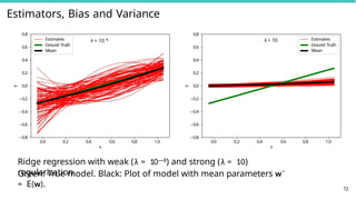
Green: True model. Black: Plot of model with mean parameters w¯
= E(w). 72
Ridge regression with weak (λ = 10—8) and strong (λ = 10)
regularization.

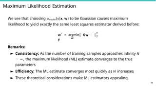
101. Estimators, Bias and Variance
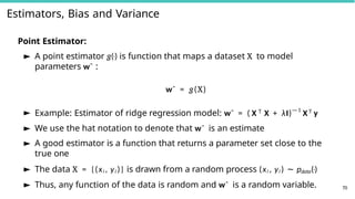
► There is a bias-variance tradeoff: E[(wˆ − w)2] = Bias(wˆ )2 + Var(wˆ )
► Or not? In deep neural networks the test error decreases with network
width!
https://www.bradyneal.com/bias-variance-tradeoff-textbooks-update
Neal et al.: A Modern Take on the Bias-Variance Tradeoff in Neural Networks. ICML Workshops,
2019.
73

102. Maximum Likelihood
Estimation

103. Maximum Likelihood Estimation
► We now reinterpret our results by taking a probabilistic
viewpoint i i
N
i=1
► Let X = {(x , y )} be a dataset with samples drawn i.i.d.
from pdata
► Let the model pmodel(y|x, w) be a parametric family of probability
distributions
► The conditional maximum likelihood estimator for w is given by
M L model
wˆ = argmax p (y|X, w)
w
iid
w
N
Y
= argmax
p i=1
model i i
(y |x , w)
w
N
Σ
= argmax log
p i=1
model i i
(y |x , w)
`
x Log-
Lik
˛
e
¸
lihood
Note: In this lecture we consider log to be the natural 75

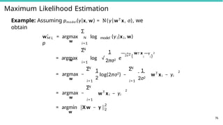
104. Maximum Likelihood Estimation
M L
w
Example: Assuming pmodel(y|x, w) = N(y|wT x, σ), we
obtain
N
Σ
wˆ = argmax log
p
model i i
(y |x , w)
w
i=1
N
Σ 1
2πσ2
= argmax log √ e
2σ 2
1 T
— w x —y
( i i )
2
w
= argmax −
i=1
N
Σ
i=1
1
2
log(2πσ2
) −
N
Σ
i=1
1
2σ2
wT
xi − yi
2
w
= argmax −
N
Σ
i=1
wT
xi − yi
2
w
= argmin X w − y
2
2
76

105. Maximum Likelihood Estimation
We see that choosing pmodel(y|x, w) to be Gaussian causes maximum
likelihood to yield exactly the same least squares estimator derived before:
w
wˆ = argmin X w −
y
2
2
Variations:
► If we were choosing pmodel(y|x, w) as a Laplace distribution, we would
obtain an estimator that minimizes the l1 norm: wˆ = argmin w X w − y 1
► Assuming a Gaussian distribution over the parameters w and
performing a maximum a-posteriori (MAP) estimation yields ridge
regression:
argmax p(w|y, x) = argmax p(y|x, w)p(w) 77

106. Maximum Likelihood Estimation
We see that choosing pmodel(y|x, w) to be Gaussian causes maximum
likelihood to yield exactly the same least squares estimator derived before:
w
wˆ = argmin X w −
y
2
2
77
Remarks:
► Consistency: As the number of training samples approaches infinity N
→ ∞, the maximum likelihood (ML) estimate converges to the true
parameters
► Efficiency: The ML estimate converges most quickly as N increases
► These theoretical considerations make ML estimators appealing