Lecture 1. Financial risk management lecture 1

Management of Financial Risk
MANG6298
Arben Kita, Management of Financial Risk, 2017

Available
This module is available for the following
programmes:
• Msc Risk and Finance
• Msc Finance

Instructor
• Arben Kita
• Office hours Wednseday 9:0 to 10:00 (email to
book a meeting with the subject of the
meeting)
• Email for appointment A.kita@soton.ac.uk
• Office building 2, room 4051

Modules Aim and Objectives
• This module aims to provide a graduate level analysis of credit, market,
liquidity, interest rate and operational risk and how these financial risks can
be measured and then managed.
• Knowledge and understanding
Having successfully completed the module, you will be able to demonstrate
knowledge and understanding of:
– The role of options and volatilities and
correlations in the management of financial risk;
– How market, interest rate and credit risk are
measured;
– How credit, market, liquidity, interest rate and
operational risks are managed;

Ground Rules
• This is an advanced course thus you are
expected to perform professional level work
• Arrive on time
• Print out the lecture notes before hand
• Switch off your mobiles or any electronic
devices
• No food
• Regularly check Blackboard & emails

Assessment
• In-class test
– One-hour test
– Three questions, one of which numerical
– Accounts for 30% of your final mark
– Week 24, Tuesday 14th March 2017, Rooms 02A/2077, 09:00-10:00
• Final exam
– Two-hour written exam
– Answer any two out of three questions
– Numerical and assay-like questions
– Accounts for 70% of your final mark

Textbook
• Hull, J. (2009) Risk Management and Financial Institutions,
Third/Fourth Edition, Wiley Finance. Recommended
• Hull, J. (2012) Options Futures and Other Derivatives, Eighth edition,
Pearson
• Bodie, Kane Marcus (2014) Investments, Tenth Global Edition,
McGraw Hill Education
• Cochrane, J.H. (2005), Asset Pricing (Princton University Press,
Princeton, N.J.)

Mean-Variance Analysis,
CAPM, APT & Risk vs Returns for
Companies

• The lecture will be divided in four parts:
- Mean-Variance analysis
- Capital Asset Pricing Model (CAPM)
- Arbitrage Pricing Theory (APT)
- Risk-Return for the companies
Structure of the lecture

Diversification of risk within a portfolio
• Labels indicate portfolio weights for Intel and Coca-Cola.
• Portfolios on the red portion of the curve are efficient.
• Those on the blue portion are inefficient – alternative portfolios
exist with a higher expected return and lower risk, i.e. to the
north-west of the blue portion.

Example: you can invest in any combination of GM, Intel and Coca-Cola.
What portfolio would you choose?
E[Rp] = (wGM x 1.08) + (wIntel x 1.32) + (wCoca-Cola x 1.75)
Var(Rp) = (wGM x 38.8) + (wIntel x 40.21) + (wCoca-Cola x 94.63) +
(2x wGM x wIntel x 16.13) + (2x wGM x wCoca-Cola x 22.43) +
(2x wIntel x wCoca-Cola x 23.99)
Variance Covariance Matrix
Stock Mean Std dev GM Intel Coca-Cola
GM 1.08 6.23 38.8 16.13 22.43
Intel 1.32 6.34 16.13 40.21 23.99
Coca-Cola 1.75 9.73 22.42 23.99 94.63

• Effect of correlation:

• Many stocks:

The straight-line relationship of risky asset and risk-
free asset
Standard deviation
Exp.
return
(%)
Rf
Diversifiable risk and undiversifiable risk
P

The straight-line relationship holds for any
combination of risky asset and risk-free asset
Standard deviation
Exp.
return
(%)
Rf
Efficient frontier
P
Intel
Coca-Cola
GM

Standard deviation
Exp.
return
(%)
Line tangential to efficient frontier gives highest rate of
trade-off between risk and return – highest price for risk.
Rf
Combinations
of a risky
portfolio and
positive
(lending) or
negative
(borrowing)
holdings of
risk-free asset
Efficient frontier
P

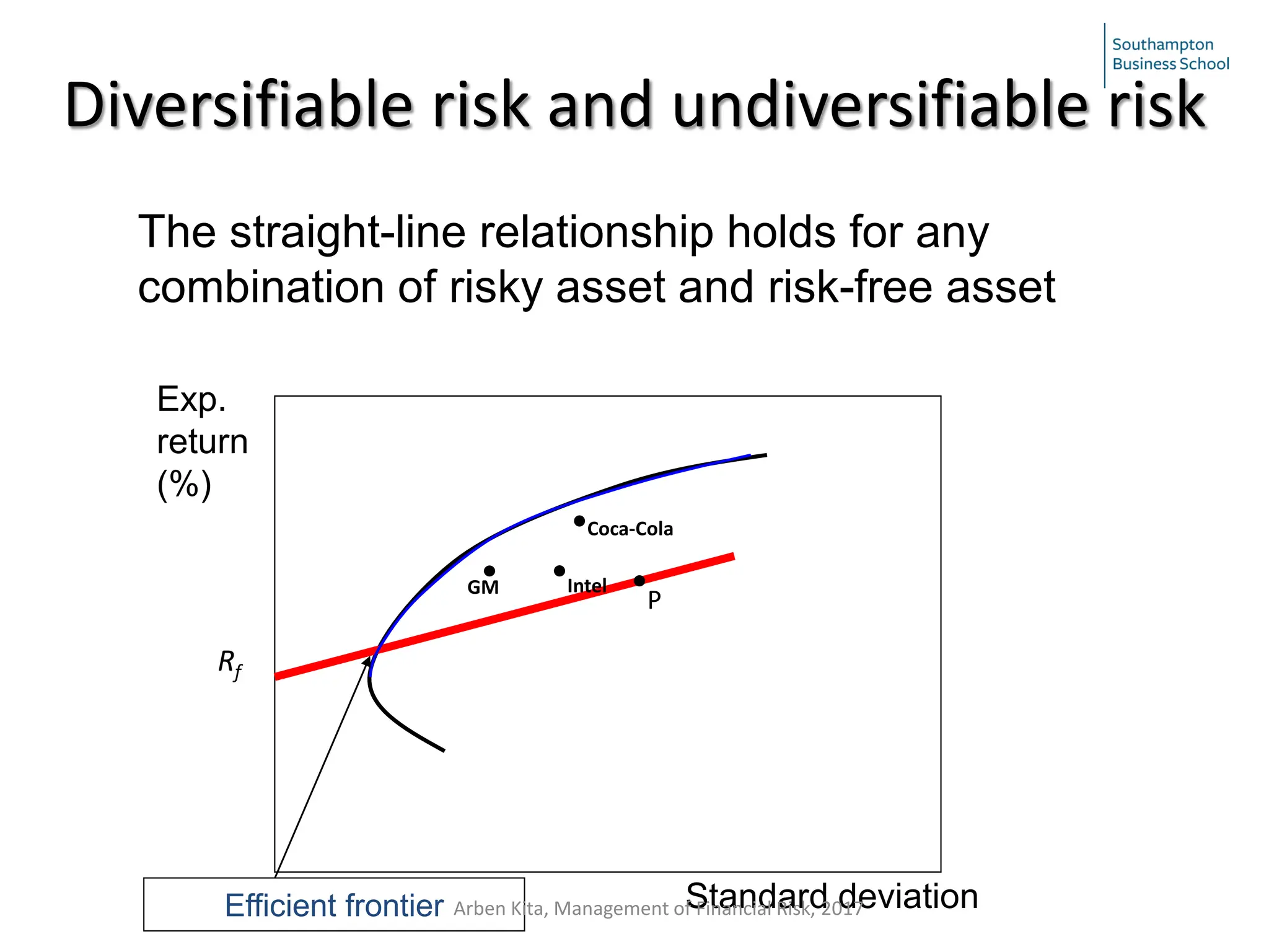
Now consider the combination (C) of a risky
portfolio (P) and a risk-free asset (with expected
return Rf), with weights w and 1-w, respectively:
)
]
[
(
)
1
(
]
[
]
[
f
P
f
f
P
C
R
R
E
w
R
R
w
R
wE
R
E
−
+
=
−
+
=
f
f R
P
2
R
2
2
P
C w
2w
+
w
+
w
= ,
2
2
)
1
(
)
1
( σ
σ
σ
σ −
−
where subscript Rf refers to the risk-free asset.
Diversifiable (unpriced, idiosyncratic) risk and
undiversifiable (priced, market) risk
and

w
=
w
=
P
C
2
P
C
σ
σ
σ
σ
⇒
2
2
w P
C σ
σ /
=
)
]
[
(
]
[ f
P
f
C R
R
E
w
R
R
E −
+
=
Since a risk-free asset has no variance and has zero covariance with
everything else, the formula for the variance collapses to:
Substitution of w into previous return expression
gives
C
P
f
P
f
C
R
R
E
R
R
E σ
σ
)
]
[
(
]
[
−
+
=
A straight-line relationship Slope
, so .

• The tangential portfolio of risky shares that (in
combination with the risk-free asset) gives the
highest rate of the trade-off between the risk and
return
• ‘Market portfolio’ (with expected return E[Rm]).

Risk Free Return =
Std. Dev. of market portfolio =
Risk
.
Rf
‘Market portfolio’
σm
Rm
Market Return =
‘Capital Market Line’ Efficient Frontier
Exp. Return
Market portfolio dominates all other risky portfolios.

• The straight-line relationship between the risk and
return of the market portfolio and the risk-free asset
is termed the Capital Market Line
• The slope of the Capital Market Line, (E[Rm]-Rf)/σm,
gives the market price of systematic risk (i.e. what
investors need to be offered in order to take on this
risk).
C
m
f
m
f
C
R
R
E
R
R
E σ
σ
)
]
[
(
]
[
−
+
=
Capital Asset Pricing Model (CAPM)

• Many stocks:
Rf
P

• Sharpe Ratio: a measure of portfolio’s risk-return trade-off,
equal to the portfolio’s risk premium divided by its volatility
• The tangency portfolio has the highest possible Sharpe ratio
of any portfolio
• Aside: Alpha is a measure of a mutual fund’s risk-adjusted
performance. The tangency portfolio also maximises the
fund’s alpha
p
f
p R
R
E
o
SharpeRati
σ
−
=
]
[

Implications of the Market Portfolio
• Efficient portfolios are combinations of the market portfolio and riskless asset
• Expected returns of efficient portfolios satisfy:
• This yields the required rate of return or cost of capital for efficient portfolios!
• Trade-off between risk and expected return
• Multiplier is the ratio of portfolio risk to market risk
• What about other (non-efficient) portfolios?
[ ] [ ]
( )
f
p
m
p
f
p R
R
E
R
R
E −
+
=
σ
σ

• Consider an individual stock, j, that is held as part
of a diversified portfolio.
• The investor only needs to be rewarded for that
part of risk which cannot be diversified because
it derives from the association between the
returns on the share and the returns of the
market as a whole (the market portfolio).

• Expressing the market-related (undiversifiable) risk in terms of standard
deviation
where ρjm is the correlation between returns of j and m,
• multiplying this by the market price of undiversifiable risk,
• and adding the result to the risk-free rate, gives the following expression
for the required return on share j:
jm
j
j
DIV
NON = ρ
σ
σ )
(
−
m
f
m R
R
E σ
/
)
]
[
( −
jm
j
m
f
m
f
j
R
R
E
R
R
E ρ
σ
σ
)
]
[
(
]
[
−
+
=

j
m
jm
m
jm
m
j
m
jm
j
β
σ
σ
σ
ρ
σ
σ
σ
ρ
σ
=
=
= 2
2
j
f
m
f
j R
R
E
R
R
E β
)
]
[
(
]
[ −
+
=
Covariance (j,m)
Variance (m)
This ratio is termed beta
The Capital Asset Pricing Model
jm
j
m
f
m
f
j
R
R
E
R
R
E ρ
σ
σ
)
]
[
(
]
[
−
+
=

• Required return is a linear function of beta.
• Beta is a measure of the extent to which the
returns on asset j are expected to co-vary with
those of the market portfolio.
• Beta is a measure of the market risk of the share.
• This market risk is the only part of risk that is
priced. Idiosyncratic risk is not priced.

Graphical representation of CAPM: Security
Market Line
Risk-free return =
Beta of market portfolio = 1.0
Exp. Return
Beta
.
Rf
‘Market portfolio’
1.0
Rm
Market return =
‘Security Market
Line’
m
jm
j
σ
ρ
σ
Systematic risk
j
f
m
f
j R
R
E
R
R
E β
)
]
[
(
]
[ −
+
=

Capital Asset Pricing Model (CAPM):
SML
• E[Ri] = Rf + βi(E[Rm] - Rf)
• Implications:
• βi = 1 => E[Ri] = E[Rm]
• βi = 0 => E[Ri] = E[Rf]
• βi < 0 => E[Ri] < E[Rf] (Why?)
Security Market Line

• The expression for beta has same form as the slope
coefficient in a univariate regression model, i.e., the
ratio of:
– the covariance between a dependent and an
independent variable and,
– the variance of the independent variable.
• In theory, beta is a forward-looking measure of how
returns are expected to co-vary in the future.
• In practice, it is often estimated by regression of a
time series of historical share returns on a matching
time series of market portfolio returns.

To apply beta in calculating the required rate of
return on a share, you need:
• Beta for that share
• The risk-free rate. (A market-wide factor, not
specific to the share)
• The excess of the required rate of return on the
market portfolio over the risk-free rate (the equity
(market) risk premium). (A market-wide factor, not
specific to the share.) There is much debate about
this. Opinion seems to be converging on something
in the region of 5-6%.

 If the beta of the share is 1.07, the risk-free
rate is 9% and the equity (market) risk
premium is 5%, the required return on the
share is
.09 + (.05 * 1.07) = .1435 (14.35%).
 Investors must be promised at least this to
induce them to hold the share.

• Things to consider:
– Choice of proxy for the market portfolio?
– What length of data set to use?
– Return interval: daily, weekly, monthly?
– Problem of thin trading which may cause sensitivity to
market to be underestimated for small stocks.
Practicalities of beta estimation

• Cisco’s returns tend to move in the same direction, but with
greater amplitude, than those of the S&P 500.
Measuring Betas
Example: Cisco

Measuring Betas
Example: Cisco
• Beta corresponds to the slope of the best-fitting line. Deviations from
it reflect diversifiable (idiosyncratic) risk.

Alpha
• Alpha measure the extra return on a portfolio
in excess of that predicted by CAPM
so that
)
(
)
( F
M
F
P R
R
R
R
E −
β
+
=
)
( F
M
F
P R
R
R
R −
β
−
−
=
α

Arbitrage Pricing Theory
• Returns depend on several factors
• We can form portfolios to eliminate the
dependence on the factors
• This leads to result that expected return is
linearly dependent on the realization of the
factors

Single Factor Model
• Returns on a security come from two
sources:
– Common macro-economic factor
– Firm specific events
• Possible common macro-economic factors
– Gross Domestic Product Growth
– Interest Rates

Single Factor Model Equation
Ri = Excess return on security
βi= Factor sensitivity or factor loading or factor
beta
F = Surprise in macro-economic factor
(F could be positive or negative but has
expected value of zero)
ei = Firm specific events (zero expected value)
𝑅𝑅𝑖𝑖 = 𝐸𝐸(𝑅𝑅𝑖𝑖) + β𝑖𝑖𝐹𝐹 + 𝑒𝑒𝑖𝑖

Multifactor Models
• Use more than one factor in addition to market return
– Examples include gross domestic product, expected
inflation, interest rates, etc.
– Estimate a beta or factor loading for each factor using
multiple regression.

Multifactor Model Equation
Ri = Excess return for security i
βGDP = Factor sensitivity for GDP
βIR = Factor sensitivity for Interest Rate
ei = Firm specific events
( ) i
iIR
iGDP
i
i e
IR
GDP
R
E
R +
+
+
= β
β

Interpretation
The expected return on a security is the sum of:
1. The risk-free rate
2. The sensitivity to GDP times the risk
premium for bearing GDP risk
3. The sensitivity to interest rate risk times
the risk premium for bearing interest rate
risk

• Arbitrage occurs if there is a zero investment portfolio with a
sure profit.
Since no investment is
required, investors can create
large positions to obtain large
profits.

• Regardless of wealth or risk aversion, investors will want an
infinite position in the risk-free arbitrage portfolio.
• In efficient markets, profitable arbitrage
opportunities will quickly disappear.

APT & Well-Diversified Portfolios
RP = E (RP) + bPF + eP
F = some factor
• For a well-diversified portfolio, eP
–approaches zero as the number of securities in the portfolio
increases
–and their associated weights decrease

No-Arbitrage Equation of APT

APT, the CAPM and the Index Model
• Assumes a well-
diversified portfolio,
but residual risk is
still a factor.
• Does not assume
investors are mean-
variance optimizers.
• Uses an observable,
market index
• Reveals arbitrage
opportunities
APT CAPM
• Model is based on an
inherently unobservable
“market” portfolio.
• Rests on mean-variance
efficiency. The actions of
many small investors
restore CAPM
equilibrium.

Multifactor APT
• Use of more than a single systematic factor
• Requires formation of factor portfolios
• What factors?
– Factors that are important to performance of the general
economy
– What about firm characteristics?

Two-Factor Model
• The multifactor APT is similar to the one-factor case.
𝑅𝑅𝑖𝑖 = 𝐸𝐸(𝑅𝑅𝑖𝑖) + β𝑖𝑖1𝐹𝐹1 + β𝑖𝑖2𝐹𝐹2 + 𝑒𝑒𝑖𝑖

Two-Factor Model
• Track with diversified factor portfolios:
– beta=1 for one of the factors and 0 for all other
factors.
• The factor portfolios track a particular source of
macroeconomic risk, but are uncorrelated with other
sources of risk.

Fama-French Three-Factor Model
• SMB = Small Minus Big (firm size)
• HML = High Minus Low (book-to-market ratio)
• Are these firm characteristics correlated with
actual (but currently unknown) systematic risk
factors?
it
t
iHML
t
iSMB
Mt
iM
i
it e
HML
SMB
R
R +
+
+
+
= β
β
β
α

The Multifactor CAPM and the APT
• A multi-index CAPM will inherit its risk factors from sources of
risk that a broad group of investors deem important enough
to hedge
• The APT is largely silent on where to look for priced sources
of risk

Risk vs Return for Companies
• If shareholders care only about systematic risk, should the
same be true of company managers?
• In practice companies are concerned about total risk
• Earnings stability and company survival are important
managerial objectives
• The regulators of financial institutions are most interested in
total risk
• “Bankruptcy costs” arguments show that that managers can
be acting in the best interests of shareholders when they
consider total risk

What Are Bankruptcy Costs?
• Lost sales (There is a reluctance to buy from a
bankrupt company.)
• Key employees leave
• Legal and accounting costs

Approaches to Bank Risk
Management
• Risk aggregation: aims to get rid of non-
systematic risks with diversification
• Risk decomposition: tackles risks one by one
• In practice banks use both approaches

Credit Ratings
Moody’s S&P and Fitch
Aaa AAA
Aa AA
A A
Baa BBB
Ba BB
B B
Caa CCC
Ca CC
C C
Investment
grade bonds
Non-investment
grade bonds

Subdivisions
• Moody’s divides Aa into Aa1, Aa2, Aa3.
• S&P and Fitch divide AA into AA+, AA, and AA−
• Other rating categories are subdivided
similarly except AAA (Aaa) and the two lowest
categories.

Lecture 1. Financial risk management lecture 1

More Related Content

Similar to Lecture 1. Financial risk management lecture 1

Recently uploaded

Lecture 1. Financial risk management lecture 1