Download to read offline


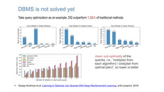

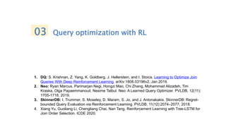
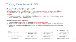
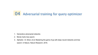
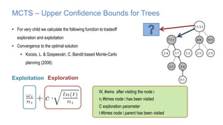
![Markov Decision Process (MDP)
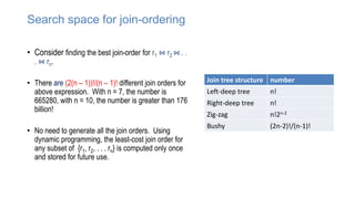
• Set of states S, set of actions A, initial state S0
• Transition model P(s,a,s’)
- P( [1,1], up, [1,2] ) = 0.8
• Reward function r(s)
- r( [4,3] ) = +1
• Goal: maximize cumulative reward in the long
run
• Policy: mapping from S to A
- (s) or (s,a) (deterministic vs. stochastic)
+1
-1
START
actions: UP, DOWN, LEFT, RIGHT
80% move UP
10% move LEFT
10% move RIGHT
1 2 3 4
1
2
3
• reward +1 at [4,3], -1 at [4,2]
• reward -0.04 for each step
• what’s the strategy to achieve max reward?
MDP solvers
- Dynamic programming
- Monte Carlo methods
- Deep Q-lerning](https://image.slidesharecdn.com/learnedoptimizer-220407161514/85/learned-optimizer-pptx-17-320.jpg)
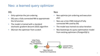
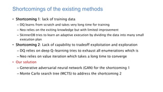
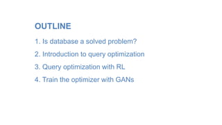
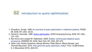
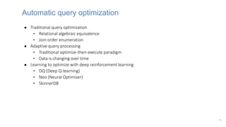
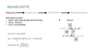
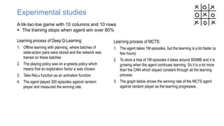
![Generative adversarial network (GAN)
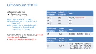
MinMax Game (Zero-sum gaming)
• Generator tries to fool discriminator (i.e. generate realistic samples)
• Discriminator tries to distinguish fake from real samples
• Each tries to minimize the objective function maximized by the other
Training set
𝑥1, ⋯ , 𝑥𝑛 ~𝑝𝑑𝑎𝑡𝑎
Discriminator 𝐷
(Binary classifier)
Generator 𝐺
min
𝐺
max
𝐷
𝑉 𝐷, 𝐺 = 𝔼𝑥~𝑝𝑑𝑎𝑡𝑎(𝑥)[log 𝐷 𝑥 ] + 𝔼𝑧~𝑝𝑧(𝑧)[log(1 − 𝐷(𝐺 𝑧 ))]
[Goodfellow et al., 2014]
1/0
𝐺𝑧
𝑥
noise 𝑧](https://image.slidesharecdn.com/learnedoptimizer-220407161514/85/learned-optimizer-pptx-25-320.jpg)
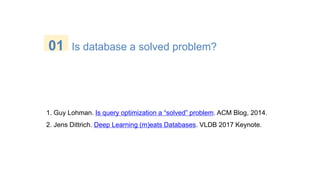
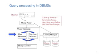
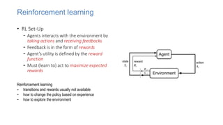
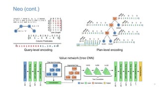
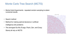
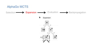
![Query optimization via adversarial training
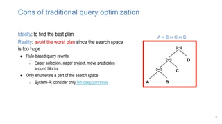
MinMax Game
• The discriminator D a cascaded joins of value network connecting all tables together
• The generator G is a cascaded series of the MCTS improved policy (i.e. generate realistic
samples)
• Each tries to minimize the objective function maximized by the other
Training set:
𝑒𝑥𝑒𝑐𝑢𝑡𝑖𝑜𝑛 𝑝𝑙𝑎𝑛𝑠: 𝑥1, ⋯ , 𝑥𝑛
Discriminator 𝐷
(Binary classifier)
Generator 𝐺
min
𝐺
max
𝐷
(𝐷, 𝐺) = 𝔼𝑥[log 𝐷 𝑥 ] + 𝔼𝑧[log(1 − 𝐷(𝐺 𝑧 ))]
1/0
𝐺𝑧
𝑥
Random plan 𝑧](https://image.slidesharecdn.com/learnedoptimizer-220407161514/85/learned-optimizer-pptx-26-320.jpg)
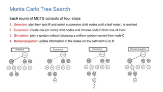
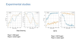


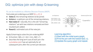
The document discusses using machine learning techniques like reinforcement learning and generative adversarial networks to improve query optimization in databases. Specifically, it summarizes work using deep Q-learning (DQ) and a neural optimizer (Neo) to learn join ordering, as well as using intra-query learning with SkinnerDB. It proposes using generative adversarial networks and Monte Carlo tree search to address shortcomings in existing approaches like lack of training data and balancing exploration vs exploitation. Generative adversarial networks could generate additional training data while Monte Carlo tree search would help optimize join ordering on a per-query basis.