This document summarizes a project to predict home insurance policy purchases from customer data using machine learning models. The authors explored a dataset of 260,753 customers to select meaningful features from 297 initial ones. They tested logistic regression, support vector machines, and gradient boosted trees on subsets of the data. Gradient boosted trees showed the best performance, with its accuracy on the test set increasing as more training data was used. The authors concluded this model was generalizing well to new data compared to the other algorithms tested.

1. UW Professional certificate in Data Science
Homesite Quote Conversion competition from Kaggle
Marciano Moreno & Javier Velázquez­Muriel
1. Introduction
The Kaggle.com website hosts competitions where the participants are asked to apply machine
learning algorithms and techniques to solve real world problems. As part of this project we are
participating in the "Homesite Quote Conversion" competition and we will work with the
Homesite dataset. Homesite chose to publish this challenge in Kaggle because they currently
do not have a dynamic conversion rate model which would allow them to be more confident that
quoted prices will lead to purchases.
The ​Homesite dataset represents the activity of a large number of customers who are interested
in buying policies from the insurance company Homesite. It contains anonymized information
about the coverage, sales, personal, property, and geographic features that the company is
using to try to predict if a customer will purchase home insurance from them. The participants in
the Kaggle competition are asked to create a model that will predict such outcome.
This project is organized as follows: The Data exploration section describes the approaches that
we followed to explore and clean the data; the Data preparation section contains the selection of
features and dimensionality reduction that we used to create the input features for the
algorithms; in the Modeling section we describe our approach for selection, training, and
refinement of the models. We conclude with some discussions and our Kaggle results.
2. Data exploration
The training dataset contains 260,753 observations, with 297 features each. It has a target
column named QuoteConversion_Flag with two possible classes: 0 and 1. The challenge asks
to predict the probability of customer conversion expressed as decimal. The test set contains
173,837 data points. The features are organized by different types:
● Fields​: No clear definition given the anonymized dataset. Probably general terms.
● Coverage​ fields: Fields related to the insurance coverage.
● Sales​ fields: Most probably, internal fields used by the company about their sales.
● Personal​ fields. Fields about the customer.
● Property​ fields. Fields about the property.
● Geographic​ fields. Geographic fields about the customer and property.

2. Unfortunately, there is no description of the features beyond that, so any field knowledge is not
possible.
Our initial data exploration consisted on visualizing the univariate distributions for each of the
numeric features in the training dataset. For each of the features we created the histogram,
density plot, the cumulative density function, and the QQNorm plot for testing of normality (Fig.
1).
Figure 1. ​Initial exploratory visualizations for the feature CoverageField1A. We created a similar plot for each feature.
After noticing certain similarity patterns occurring in the distributions of many of the features, we
decided to analyze in further depth those features. We employed a number of heuristics for
such task: unique value summarization, high data concentration (low standard deviation), and
unique sequential values. Our analysis identified that many of the "suspicious" features had
integer values ranging from ­1 to 25. Although is difficult to tell for sure, we inferred that most
probably those features were in fact of categorical nature. Based on this criterion, it turned out
that most of the fields should be treated as categorical (Supplementary section S.2).

3.
3. Data preparation and feature selection
3.1 Data preparation
When we compared the values for the categorical features in the train dataset with their values
in the test set we discovered that some features did not have the same values among these
datasets. In particular, the test dataset contained levels not found in the train dataset. Although
it is true that a model built with features whose values are not found in the train set will likely
exhibit degraded performance, the extent of the problem was fairly minor, with at most 2 missing
values per feature. We therefore kept the problematic features and solved the issue by
enforcing R to consider the new levels. We discarded PropertyField6 and GeographicField10A
because they only contained one value, and PersonalField84 and PropertyField29 because
more than 70% of the values were missing. We converted dates to 3 numeric variables (Day,
Month, Year). After data exploration and preparation, we were left with 245 categorical features
and 50 numeric ones.
3.2 Feature selection
We approached the problem of feature selection using two different techniques: Dimensionality
reduction and feature prioritization. For dimensionality reduction we considered a number of
algorithms: Principal Component Analysis (PCA), Multiple Correspondence Analysis (MCA), and
Factor Analysis for Mixed Data (FAMD). All these algorithms have as purpose to reduce the
dimension of the feature space by combining the original features to create new features. The
newly created features are ranked by the amount of the variance present in the original features
that they are able to explain. We employed the versions of the algorithms from the R package
FactoMineR [1]. For categorical feature prioritization we used the ChiSquareSelector filtering
algorithm from the R package FSelector [2]. In the case of categorical feature prioritization, the
dimensionality of the dataset does not change by the application of the method, rather it
empowers the analyst to determine which features to integrate or discard from the model.
For dimensionality reduction we first applied FactorMineR PCA on all the 260,073 observations
and 292 features (we excluded date/time related features). Only the 50 numeric features are
employed by the algorithm, with categorical features employed only aiding in the interpretation
of the results. The PCA decomposition produced 50 eigenvectors and and 50 eigenvalues. The
first eigenvalue (dimension 1) explained 16.85% of the variance and the second one 13.55%
(Fig. 2). The first 30 PCA dimensions explained 99% of the variance.

4.
Figure 2​. ​Left: ​Factor map of the PCA decomposition of the 50 numeric features. All categorical features as
supplementary variables. ​Right: ​PCA Individual Factor Map (all observations, categorial features as supplementary
variables).
Next we applied FactoMineR’s MCA method, suitable for categorical features. Treating all
observations at once was not possible with our computers, so we proceed by repeating the
application of MCA 10 times, each applied on a random 10% of the observations. The results
(eigenvectors and eigenvalues of the decomposition) were stable and similar in all cases.
Unfortunately, the performance was poor: Each of the first few eigenvalues only explained ~1%
of the variance. We thus discarded the use of MCA. Lastly, we applied FAMD. This method
seemed adequate to our case, as the algorithm can treat numeric and categorical features at
the same time. A test run with 50,000 observations showed that FAMD had the same poor
performance as MCA, so we didn't pursue further its use.
For categorical value prioritization we applied the ChiSquareSelector filtering algorithm. The
algorithm performs a ᵭ​2​
­test for each of the categorical features against the target feature. The
features are sorted by their importance, allowing to readily identify the features that have more
predictive value. We arbitrarily set a cutoff for the number of variables to use at 145 because at
that point the value of the importance was already ⅛ of the importance of the most predictive
feature.

5. In conclusion: after the dimensionality reduction and feature selection we were left with 10
continuous variables obtained after PCA dimensionality reduction and the first 145 most
predictive categorical values for the first iteration of the modeling and evaluation cycle.
4. Modeling
4.1 Analytic problem to be solved and methodology
The Homesite Quote Conversion challenge is a supervised learning probabilistic classification
task. The participants are asked to create a model which determines the probability that a
customer will purchase the Homesite insurance policy for each of the observations in the test
dataset. We therefore applied the standard procedure for supervised learning. First, we
randomly splitted our initial dataset of 260,073 observations into three separate datasets:
training (156,468 observations, ~60% of the initial dataset), testing (52,397 observations, ~20%)
and cross­validation (51,208 observations, ~20%). The intended use for each of the datasets
was as follows:
● The training dataset was used to train a specific instance of a family of algorithms.
● The test dataset was used to diagnose the behavior of each of the algorithms and
optimize its hyperparameters.
● The cross­validation dataset was used to evaluate the performance of the models
created after training and hyperparameter optimization.
We chose to try three algorithms: logistic regression (LR) with lasso/ridge regularization, support
vector machines (SVM), and gradient boosted trees (GBT) for the following reasons:
● logistic regression is a well known algorithm that assumes linear relationships and it is a
simple try­first model that can work well if the data have linear structure. We used the R
package glmnet [3].
● SVM is considered one of the best off­the­shelf machine learning algorithms and a
candidate for good performance. We used the R package e1071 [4].
● GBT has built a reputation of being a state­of­the­art, powerful algorithm and has been
used to win several Kaggle competitions. We used the R package xgboost [5].
For each of the algorithms we proceeded by building learning curves to evaluate run­time and
classification performance, together with diagnosing bias/variance issues. We optimized the
hyperparameters of the best algorithms using the R package caret [6] and standard functions
provided by the e1071 SVM package.
4.2 Learning curves

6. We built the learning curves for all algorithms by training the model with an increasing fraction of
observations from the training dataset and evaluating the performance on the test dataset using
the F­measure defined as follows:
F = 2Precision+Recall
Precision ∙ Recall
For logistic regression the learning curves (Fig. 3) for both 20 and 40 features showed rather
poor performance for the classifier, with values F ≈ 0.64 for the training set and F ≈ 0.63 for the
test set after using 15% of the observations. Such poor performance that does not change by
increasing the number of training examples was indicative of high­bias. The performance of the
classifier did not improve after using 60 features (Fig. 4), further confirming the presence of
high­bias, either due to non­informative features or LR not performing well. We thus decided to
stop adding features and discard LR algorithm due the increasing running times and the lack of
learning improvement.

7. Figure 3. Learning curves for the logistic regression (LR) algorithm from glmnet. y­axis: F­measure for the
performance of the classifier. ​Upper left: Curves created with the first 20 predictive features (10 PCA features, 10
most informative categorical features) and up to 50% of the training dataset. ​Upper right​: Curves created with the
first 40 features (10 PCA, 30 most informative categorical). ​Lower left: Curves created with the first 60 features (10
PCA, 50 most informative categorical) and up to 15% of the observations in the training dataset.
The learning curves for GBT (Fig. 4) using 20, 40, and 60 features and default parameters
showed the same high­bias regime observed for LR: Similar values of F for the train and test
sets that do not improve by adding new observations. For GBT though we managed to run the
algorithm employing all variables and 100% of the training examples. Now the learning curves
(Fig.4, lower right) showed improved values of the F­measure and also a trend of F increasing
for the test set as the number of training examples increased. An indication that GBT was
generalizing well.
Figure 4. Learning curves for the Gradient Boosted Trees (GBT) algorithm from xgboost.. y­axis: F­measure for the
performance of the classifier. ​Upper left: Curves created with the first 20 predictive features (10 PCA features, 10
most informative categorical features) and up to 50% of the training dataset. ​Upper right​: Learning curves created
with the first 40 features (10 PCA, 30 most informative categorical) up to 50% of the training dataset. ​Lower left:

8. Curves created with the first 60 features (10 PCA, 50 most informative categorical) and up to 100% of the training
dataset. ​Lower right: ​Curves created with all the 175 selected features up to 100% of the training dataset.
We also built learning curves for a SVM model4 of C­classification type with radial kernel (Fig.
5). Here we measured performance with the accuracy measure from the e1071 R package
(defined as the percentage of data points in the main diagonal of the confusion matrix. The
learning curves for SVM showed again a high­bias regime: For 20 features, the maximum
diagonal was ~0.865 at 15% of the training points and did not exhibit improvement with more
training samples. Adding more features did not help. Especially relevant were the curves for 50
features (Fig. 5, lower right), as they show the characteristic shape of the high bias regime
previously observed for LR (Fig. 3, lower left) and GBT (Fig 4, lower left).

9.
Figure 5. Learning curves for the Support Vector Machine (SVM). Diagonal as the performance of the classifier with
up to 30% of the training dataset for all cases. ​Upper lef​t: Curves created with the first 20 predictive features (10
PCA and 10 categorical). ​Upper right​: Learning curves created with the first 30 predictive features (10 PCA, 20
categorical). ​Lower left​: Learning curves created with the first 40 predictive feature (10 PCA and 30 categorical).
Lower right​: Learning curves created with the first 50 predictive features (10 PCA and 40 categorical).
We diagnosed the source of bias by plotting bias/variance curves, which depict the variation in a
performance measure as new features are added to the models, for both SVM and GBT (Fig.
6). The curves for SVM (Fig. 6, left) are the result of evaluating multiple models (represented in
the horizontal axis), each with an increasing quantity of factors. The SVM models with the lower
number of factors showed a low variance regime, while the SVM models with the higher number
of factors showed high variance regime: that training and test sets started to diverge for more
than 20 features and the difference kept increasing. This was not apparent in the initial plots of
accuracy because the range of features was smaller than the one used in the Bias/Variance
plots. On the other hand, GBT kept improving performance with added features with no
indication of entering into a high variance regime (Fig. 6, right).
Figure 6. ​Left: ​Bias/Variance curve for SVM trained with ~10% of the training samples and up to 80 the features. The
performance measure is the error rate, defined as (FP+FN)/(TP+TN+FP+FN). ​Right: Bias/Variance curve for GBT
trained with ~50% of the training samples and up to all of the original features.
4.3 Model hyperparameters optimization

10.
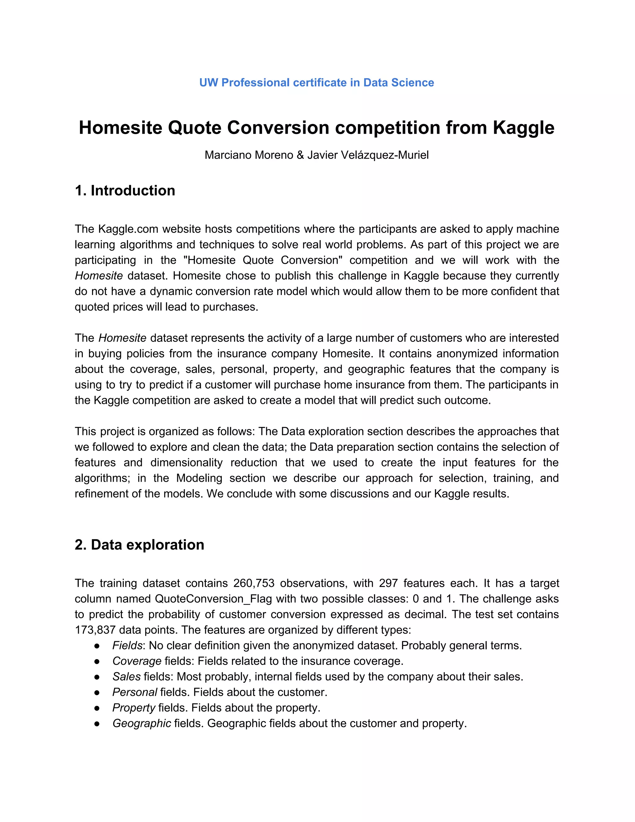
The learning and bias/variance curves for GBT indicated that the combination of the selected
features and the GBT algorithm could work well for our case. We therefore proceeded to find
the best possible GBT model by optimizing its hyperparameters:
● max_depth​: The maximum depth of the trees to built during the learning stages. High
values with result in overfitting.
● nrounds​: The number of passes over the data that GBT will do. The more the passes,
the better the fit between between predictions and ground truth for the training dataset.
Higher values will result in overfitting.
● eta​: A "shrinkage" step size varying from 0 to 1 used to control boosting. After each
boosting step, eta is used to shrink the weights of new features to make the boosting
process more/less conservative. Higher values will not shrink, enhancing the boosting
step but possible overfitting.
We ran the optimization using the R package caret [6]. The optimization involved 5­fold cross
validation employing the entire training dataset (Fig. 7, left). The test set had similar results
(Fig.7, right).
Figure 7. ​Left: Value of the area under the ROC curve (AUC) as a function of the GBT model parameters. The best
model corresponds to max_depth=5, nrounds=100 and eta=0.3, with AUC=0.961. ​Right​: ROC curve of the
predictions for the test set (the test set was not used during the optimization). AUC=0.959.
We optimized the SVM results in stages, using the tune() method from e1071. The first result
had optimal parameters C = 1 and gamma = 0.00729. Upon review of the results, a second
SVM optimization was performed using our initial Homesite dataset (10 PCA features, 145
categorical features) and 4% of the training samples. The search grid for the optimization of the
hyperparameters was gamma = c(0.000003, 0.00003, 0.0003, 0.0003979308, 0.003, 0.03), and
a cost = c(0.1, 1, 10, 100, 1000). We obtained the optimal model for cost = 10 and gamma =

11. 0003979 (Fig. 8), with values for the performance metrics F­Measure = 0.666 and accuracy =
0.94.
Figure 8.​ ROC curve for the optimal SVM model (cost = 10, gamma = 0.0003979). The best model had AUC=0.75.
4.4 Model refinement and Kaggle submissions
We created our models based on the approach described in sections 4.1­4.3. Once that we
considered a model final, we created predictions for the blind test dataset provided by Kaggle
and submitted them for rating. We repeated this procedure of model creation, hyperparameter
optimization, and submission to Kaggle multiple times (Table 1).
Table 1. ​History of Kaggle submissions
Date AUC Position Algor. Parameters Features Notes
2015­12­02 0.95566 485/611 GBT max_depth=5,nround
s=30, eta=0.3
PCA, Chi­Squared
2015­12­03 0.96238 415/635 GBT max_depth=5,nround
s=100, eta=0.3
30 PCA features, all
categorical
2015­12­04 0.96339 401/643 GBT max_depth=5,
norunds=500, eta=0.3
30 PCA features, all
categorical
2015­12­07 0.37341 N/A SVM cost = 100, gamma =
0.03
20 PCA features, all
categorical

12. Discussion
We approached this project with the intention of following a rational approach to all the parts of
building a good model rather than concentrating on trying a large number of algorithms. We
employed a large percentage of the time analyzing the features and making sure that we had
correctly identified their type. We also explored in great detail the process of feature selection
and dimensionality reduction. Ours efforts during modeling seeked to find how the selected
algorithms were learning and also diagnose the sources of bias or variance. In the case of the
SVM we learned it has a strong dependence to parameter configuration, in addition to having
particular requirements for metadata [7] (using binarized features, instead of categoricals).
Based on this approach we submitted multiple results to Kaggle for GBT and SVM. Our top
performance was a very good value of the area under the ROC curve = 0.96339, but not
enough to make it to the top of the leaderboard! As of today the model in the first place has an
AUC = 0.96990. We plan to continue working on this challenge on an ongoing basis and will
address these points accordingly.
Contributions
Marciano 1) created the exploratory univariate numerical and the distributions plots, 2) applied
PCA, MCA and FAMD for dimensionality reduction, and 3) trained and tuned the SVM models.
Javier 1) analyzed in detail the features to discover which ones should be categorical, 2)
cleaned and prepared the data, 3) applied the ChiSquaredSelector algorithm for categorical
variables prioritization, and 4) trained the LR and GBT models.
Code
Our code is available on github:
https://github.com/javang/HomesiteKaggle
References
1. FactorMineR: ​http://factominer.free.fr/

13. 2. FSelector: ​https://cran.r­project.org/web/packages/FSelector/index.html
3. glmnet: ​https://cran.r­project.org/web/packages/glmnet/index.html
4. e1071: ​https://cran.r­project.org/web/packages/e1071/index.html
5. xgboost: ​https://cran.r­project.org/web/packages/xgboost/index.html
6. caret: ​https://cran.r­project.org/web/packages/caret/index.html
7. A practical guide to support vector classification:
http://www.csie.ntu.edu.tw/~cjlin/papers/guide/guide.pdf
Supplementary Material
S.1 Feature treatment
For completeness, we describe below the treatment that we used for each of the features:
Fields:
● We treated the features Field6, Field7, and Field12 as categorical, and the rest of them
as numeric.
Coverage fields:
● Coverage Fields 1A, 1B, 2A, 2B, 3A, 3B, 4A, 4B, 5A, 5B, 6A, 6B, 8, 9, 11A, and 11B
were treated as categorical features, and the rest as numeric.
Sales fields:
● SalesFields 1A, 1B, 2A, 2B, 3 , 4 , 5 , 6 , 7 , and 9 were treated as categorical features,
and the rest as numeric.
Personal fields:
● PersonalFields 1, 2, 4A, 4B, 6, 7, 8, 9, 10A, 10B, 11, 12, 13, 15, 16, 17, 18, 19, 20,
22, 28, 29, 34, 35, 36, 37, 38, 39, 40, 41, 42, 43, 48, 53, 58, 59, 60, 61, 62, 63, 64, 65,
68, 71, 72, 73, 78, and 83 were treated as categorical features, and the rest as numeric.
Property fields
● Property Fields 1A, 1B, 2A, 2B, 3, 4, 5, 7, 8, 9, 10, 11A, 11B, 12, 13, 14, 15, 16A, 16B,
17, 18, 19, 20, 21A, 21B, 22, 23, 24A, 24B, 26A, 26B, 27, 28, 30, 31, 32, 33, 34, 35, 36,
37, 38, 39A, and 39B were treated as categorical features, and the rest as numeric.

14.
Geographic fields:
● Geographic Fields 1A, 1B, 2A, 2B, 3A, 3B, 4A, 4B, 5A, 5B, 6A, 6B, 7A, 7B, 8A, 8B, 9A,
9B, 10B, 11A, 11B, 12A, 12B, 13A, 13B, 14A, 14B, 15A, 15B, 16A, 16B, 17A, 17B, 18B,
19A, 19B, 20A, 20B, 21A, 21B, 22A, 22B, 23A, 23B, 24A, 24B, 25A, 25B, 26A, 26B,
27A, 27B, 28A, 28B, 29A, 29B, 30A, 30B, 31A, 32A, 32B, 33A, 33B, 34A, 34B, 35A,
35B, 36A, 36B, 37A, 37B, 38A, 38B, 39A, 39B, 40A, 40B, 41A, 41B, 42A, 42B, 43A,
43B, 44A, 44B, 45A, 45B, 46A, 46B, 47A, 47B, 48A, 48B, 49A, 49B, 50A, 50B, 51A,
51B, 52A, 52B, 53A, 53B, 54A, 54B, 55A, 55B, 56A, 56B, 57A, 57B, 58A, 58B, 59A,
59B, 60A, 60B, 61A, 61B, 62A, 62B, 63, 64 were treated as categorical features, and the
rest as numeric.

References

1. FactorMineR: http://factominer.free.fr/](https://image.slidesharecdn.com/515fe0fb-6e12-4218-804c-01ef1af94c4a-151218194518/75/KnowledgeFromDataAtScaleProject-12-2048.jpg)