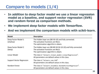
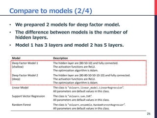
The document presents a deep factor model for forecasting stock returns using deep learning and layer-wise relevance propagation (LRP). It discusses the challenges in traditional forecasting methods and introduces a unified framework for predicting stock returns while ensuring model interpretability. The authors validate their model against various benchmarks, demonstrating its superior accuracy and profitability in stock price predictions.

1. Deep Factor Model
EXPLAINING DEEP LEARNING DECISIONS
FOR FORECASTING STOCK RETURNS
WITH LAYER-WISE RELEVANCE PROPAGATION
KEI NAKAGAWA, TAKUMI UCHIDA AND TOMOHISA
AOSHIMA

2. Contents
1.Introduction
2.Deep Factor Model
3.Experiment
4.Interpretation of Deep Factor Model
5.Conclusion
2

3. Contents
1.Introduction
2.Deep Factor Model
3.Experiment
4.Interpretation of Deep Factor Model
5.Conclusion
3

4. Background (1/5)
• To forecast stock price, we use time-series data or
cross-section data.
• But, It is difficult to forecast stock prices with time-
series data.
• On the other hand, to some extent, the cross
section of stock returns are predictable.
4
Time Series
CrossSection

5. Background (2/5)
• “Factor” explains stock prices with cross-section
data.
• In general, multifactor model explains the stock
returns through multiple factors.
• There are two uses of the multifactor model.
Return model
To enhance the return by predicting the future value of
the factors.
Risk model
To control the risk by capturing the major sources of
correlation among stock returns.
5

6. Background (3/5)
• In the academic field of finance, Fama-French
three-factor model is used.
• Since three-factor model has been presented, 316
factors have been discovered so far.
• However, It's difficult to verified 316 factors
simultaneously due to “The curse of
dimensionality”.
• Furthermore, financial markets are nonlinear, but
these models including Fama-French three-factor
model are almost linear.
6

7. Background (4/5)
• Because of high dimensionality and non linearity,
application of machine learning is active in the field
of stock price forecasting.
• Especially deep learning is applied in various fields
with high precision.
• However it has significant disadvantages such as a
lack of transparency and limitations to the
interpretability of the prediction.
7
…
…
…
…
…

8. Background (5/5)
• From the viewpoint of Fiduciary duty in asset
management companies, explanation of the model
is very important.
• Furthermore General Data Protection Regulation
also includes “Transparency principle” and
“Accountability principle”.
8
…
…
…
…
…

9. Our research
• We propose to represent a return model and risk
model in a unified manner with deep learning.
• We implement deep learning to predict stock
returns with various factors as a return model.
• And, we present the application of layer-wise
relevance propagation to decompose attributes of
the predicted return as a risk model.
• We called this model as Deep Factor Model.
9

10. Contents
1.Introduction
2.Deep Factor Model
3.Experiment
4.Interpretation of Deep Factor Model
5.Conclusion
10

11. Overview (1/2)
• This figure shows the image of implementation of
deep learning to predict stock returns with various
factors.
• It corresponds to the “Return model” of the
multifactor model.
11
…
Output
(Predicted Stock Return)
…
…
…
Forward Propagation (return model)
Input
(Factor Exposure)
…

12. Overview (2/2)
• This figure shows the application of LRP to
decompose attributes of the predicted return.
• It corresponds to the “Risk model” of the
multifactor model.
12
…
Output
(Predicted Stock Return)
…
…
…
Forward Propagation (return model)
Layer-wise Relevance Propagation (risk model)
Input
(Total Relevance)
Input
(Factor Exposure)
…
Output
(Relevance Decomposition)

13. What is LRP? (1/2)
• Layer-wise Relevance
Propagation is an inverse
method that calculates the
contribution of the prediction
made by the network.
• LRP aims to find a relevance
score 𝑹 𝒅 for each vector
element in layer such that the
following equation holds.
13
321
1
2
3
4
5
6
𝑤56
𝑤46
𝑤14
𝑤15
𝑤35
𝑧4
𝑧5
Forward Propagation
Layer-wise Relevance Propagation
𝑅4
(2)
𝑅1
(1)
𝑅6
(3)
𝑅5
(2)
𝑅2
(1)
𝑅3
(1)
𝑧46
2,3
𝑧56
2,3
𝑧14
1,2
𝑧35
1,2
Layer l
𝑓 𝑥 = 𝑅6
(3)
= 𝑅5
(2)
+ 𝑅4
(2)
= 𝑅3
(1)
+ 𝑅2
(1)
+ 𝑅1
(1)

14. What is LRP? (2/2)
• LRP uses weights and
activated values obtained by
the network.
• Then we back-propagate the
output values to the input
layer.
• As a result, we can see which
input values contribute to an
output.
14
321
1
2
3
4
5
6
𝑤56
𝑤46
𝑤14
𝑤15
𝑤35
𝑧4
𝑧5
Forward Propagation
Layer-wise Relevance Propagation
𝑅4
(2)
𝑅1
(1)
𝑅6
(3)
𝑅5
(2)
𝑅2
(1)
𝑅3
(1)
𝑧46
2,3
𝑧56
2,3
𝑧14
1,2
𝑧35
1,2
Layer

15. How to compute LRP? (1/2)
• I will explain the calculation
method of LRP with the toy
model.
• Focus on 𝑅6
(3)
.
• 𝑅6
(3)
is connected only to 𝑅4
(2)
and
𝑅5
(2)
.
• Because the relevance score of
each layer is the same value,
the influence of 𝑅6
(3)
is
distributed 𝑅4
(2)
and 𝑅5
(2)
.
15
321
1
2
3
4
5
6
𝑤56
𝑤46
𝑤14
𝑤15
𝑤35
𝑧4
𝑧5
Forward Propagation
Layer-wise Relevance Propagation
𝑅4
(2)
𝑅1
(1)
𝑅6
(3)
𝑅5
(2)
𝑅2
(1)
𝑅3
(1)
𝑧46
2,3
𝑧56
2,3
𝑧14
1,2
𝑧35
1,2
Layer
𝑅4
(2)
=
𝑧46
2,3
𝑧46
2,3
+ 𝑧56
2,3
𝑅6
(3)

16. How to compute LRP? (2/2)
• Distribution ratio is calculated
by each weight and activated
value.
• We get 𝑧56
(2,3)
and 𝑧46
(2,3)
as
following equations.
• By repeating the same
calculation to the input layer,
we can calculate each
contribution of input layer.
16
321
1
2
3
4
5
6
𝑤56
𝑤46
𝑤14
𝑤15
𝑤35
𝑧4
𝑧5
Forward Propagation
Layer-wise Relevance Propagation
𝑅4
(2)
𝑅1
(1)
𝑅6
(3)
𝑅5
(2)
𝑅2
(1)
𝑅3
(1)
𝑧46
2,3
𝑧56
2,3
𝑧14
1,2
𝑧35
1,2
Layer
𝑧56
2,3
= 𝑤56 𝑧5
𝑧46
2,3
= 𝑤46 𝑧4

17. Contents
1.Introduction
2.Deep Factor Model
3.Experiment
4.Interpretation of Deep Factor Model
5.Conclusion
17

18. Description of dataset
• We used the constituents of TOPIX
Index. This is one of most popular
indices in Japan.
• We used the data from April 2006
to February 2016. The total
number of companies are 2046.
• We used five factors: Risk, Quality,
Momentum, Value, and Size.
• These factors are divided into
descriptors.
18
Factor Descriptors
Risk 60VOL
BETA
SKEW
Quality ROE
ROA
ACCRUALS
LEVERAGE
Momentum 12-1MOM
1MOM
60MOM
Value PSR
PER
PBR
PCFR
Size CAP
ILLIQ

19. How to preprocess
• Our problem is to find a
predictor f(x) of an output
Y.
• X is the descriptors of
previous month, 3 month, 6
month , 9 month, and 12
month ago.
• Therefore, the total number
of X is 80.
• The Y is the next month’s
stock return.
19
Target month
3 month ago
6 month ago
9 month ago
12 month ago
16 descriptors
5units
Next month
Stock return

20. Compare to models (1/4)
• In addition to deep factor model we use a linear regression
model as a baseline, and support vector regression (SVR)
and random forest as comparison methods.
• We implement deep factor models with Tensorflow.
• And we implement the comparison models with scikit-learn.
20
Model Description
Deep Factor Model 1
(shallow)
The hidden layer are {80-50-10} and fully connected.
The activation functions are ReLU.
The optimization algorithm is Adam.
Deep Factor Model 2
(deep)
The hidden layer are {80-80-50-50-10-10} and fully connected.
The activation functions are ReLU.
The optimization algorithm is Adam.
Linear Model The class is “sklearn.linear_model.LinearRegression”.
All parameters are default values in this class.
Support Vector Regression The class is “sklearn.svm.SVR”.
All parameters are default values in this class.
Random Forest The class is “sklearn.ensemble.RandomForestRegressor”.
All parameters are default values in this class.

21. Compare to models (2/4)
• We prepared 2 models for deep factor model.
• The difference between models is the number of
hidden layers.
• Model 1 has 3 layers and model 2 has 5 layers.
21
Model Description
Deep Factor Model 1
(shallow)
The hidden layer are {80-50-10} and fully connected.
The activation functions are ReLU.
The optimization algorithm is Adam.
Deep Factor Model 2
(deep)
The hidden layer are {80-80-50-50-10-10} and fully connected.
The activation functions are ReLU.
The optimization algorithm is Adam.
Linear Model The class is “sklearn.linear_model.LinearRegression”.
All parameters are default values in this class.
Support Vector Regression The class is “sklearn.svm.SVR”.
All parameters are default values in this class.
Random Forest The class is “sklearn.ensemble.RandomForestRegressor”.
All parameters are default values in this class.

22. Compare to models (3/4)
• We use the same data set for comparison methods.
• We uses the default value of scikit-learn for
comparison models’ parameters.
22
Model Description
Deep Factor Model 1
(shallow)
The hidden layer are {80-50-10} and fully connected.
The activation functions are ReLU.
The optimization algorithm is Adam.
Deep Factor Model 2
(deep)
The hidden layer are {80-80-50-50-10-10} and fully connected.
The activation functions are ReLU.
The optimization algorithm is Adam.
Linear Model The class is “sklearn.linear_model.LinearRegression”.
All parameters are default values in this class.
Support Vector Regression The class is “sklearn.svm.SVR”.
All parameters are default values in this class.
Random Forest The class is “sklearn.ensemble.RandomForestRegressor”.
All parameters are default values in this class.

23. Compare to models (4/4)
• We use the latest 60 sets of training data from the
past 5 years.
• We roll the window forward by 1 month and repeat
120 times.
23
…
60 months as training
1 month as test
…
…
…
…
…
120 times
from April 2006

24. Result (1/5)
• The result of validation is the table 4.
• We calculated root-mean-squared error (RMSE) and
mean-absolute error (MAE) as the accuracy
measure.
• We also calculated annualized return, volatility and
Sharpe ratio as the profitability measure.
24

25. Result (2/5)
• In terms of MAE and RMSE, the shallow Deep Factor
Model 1 is the best accuracy.
25

26. Result (3/5)
• On the other hand, in terms of profitability, “Return”
is Model 1 and “Volatility” is the best value for
Random Forest.
26

27. Result (4/5)
• But in the overall evaluation Sharpe Ratio, Model 2
is the best.
27

28. Result (5/5)
• In any case, we find that both models 1 and 2
exceed the baseline model, SVR, and random forest
in terms of accuracy and profitability.
• From this result, we can see that the deep learning
model is effective for stock price prediction using
market index value.
28

29. Contents
1.Introduction
2.Deep Factor Model
3.Experiment
4.Interpretation of Deep Factor Model
5.Conclusion
29

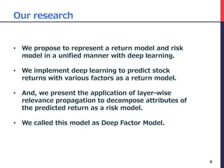
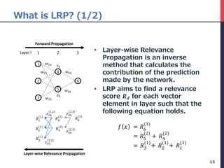
30. Calculation process of LRP (1/5)
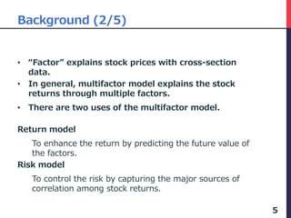
• There are 5 steps in this procedure.
• We use the data as of February 2016 to illustrate
the process.
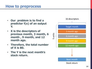
• Step 1, we calculate LRP for each 80 variables.
30
this month … -12 month
Company_ID yyyymm Risk_60VOL Risk_BETA Quality_ROE … Value_EP Value_BR Value_PCFR
c0001 201602 0.110 0.837 0.822 … 0.021 0.067 0.001
c0002 201602 0.111 0.809 0.823 … 0.018 0.058 0.010
c0003 201602 0.108 0.785 0.799 … 0.020 0.066 0.001
… … … … … … … … …
[Step 1] Calculate LRP of each sample of only 201602(latest) yyyymm set

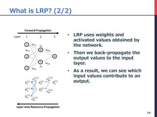
31. Calculation process of LRP (2/5)
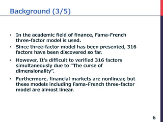
• In Step 2, We aggregate the descriptors to 5
factors.
31
[Step 2] Group Calculated LRP of each descriptor by 5 Factor.
this month … -12 month …
Company_ID yyyymm Risk_60VOL Risk_BETA Quality_ROE … Risk_60VOL Risk_BETA Quality_ROE …
c0001 201602 0.110 0.837 0.822 … 0.021 0.067 0.001 …
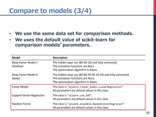
c0002 201602 0.111 0.809 0.823 … 0.018 0.058 0.010 …
c0003 201602 0.108 0.785 0.799 … 0.020 0.066 0.001 …
… … … … … … … … … …
sum of all month
Company_ID yyyymm Risk_* Quality_* Momentum_* Value_* Size_*
c0001 201602 1.318 8.366 2.091 0.418 0.209
c0002 201602 1.222 9.708 4.854 0.971 0.194
c0003 201602 1.400 7.068 2.356 0.471 0.094
… … … … … … …

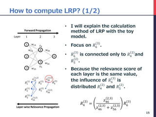
32. Calculation process of LRP (3/5)
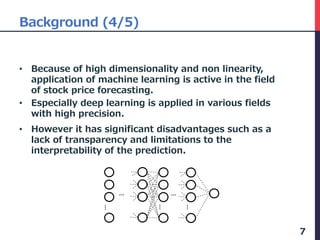
• Step 3, we convert this to a percentage.
• The result is the following table.
• This expresses the percentage that affected that
prediction.
32
[Step 3] Convert the summed LRP to percentage.
sum of all month
Company_ID yyyymm Risk_* Quality_* Momentum_* Value_* Size_*
c0001 201602 11% 67% 17% 3% 2%
c0002 201602 7% 57% 29% 6% 1%
c0003 201602 12% 62% 21% 4% 1%
… … … … … … …

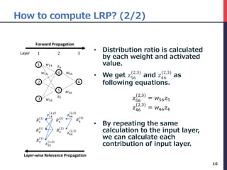
33. Calculation process of LRP (4/5)
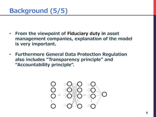
• Step 4, samples are sorted in descending order of
predicted return first.
• We will extract Highest predicted company and
company set of Top Quantile.
33
[Step 4] Sort descending order by predicted next month return.
sum of all month predicted
return of next
month
Company_I
D yyyymm Risk_* Quality_* Momentum_* Value_* Size_*
c0871 201602 0.076 0.652 0.227 0.030 0.015 0.87
c1981 201602 0.084 0.654 0.178 0.056 0.028 0.74
c0502 201602 0.215 0.570 0.127 0.051 0.038 0.71
c0070 201602 0.152 0.674 0.130 0.022 0.022 0.68
… … … … … … … …
c1788 201602 0.220 0.610 0.171 0.000 0.000 -0.92
c0834 201602 0.138 0.646 0.185 0.000 0.031 -0.94
c0043 201602 0.131 0.571 0.214 0.048 0.036 -1.05
Companies in top quantile

34. Calculation process of LRP (5/5)
• Step 5, we compare the two extracted data.
• Top quantile's company's factor score is average.
• By doing this, we can see which factor was affected
by the company that was expected to have a high
Return value.
34
[Step 5] Compaire between Highest predicted company VS Average of Top Quantile.
sum of all month
segment Risk_* Quality_* Momentum_* Value_* Size_*
Highest Company
(c0871)
0.23 0.31 0.15 0.28 0.03
Average of Top
Quantile
0.16 0.33 0.15 0.30 0.05

35. Interpretation (1/5)
• The figure shows which factor contributed to the
prediction in percentages with LRP.
• The quality and value factors account for more than
half of the contribution to both the stock return and
quintile portfolio.
35

36. Interpretation (2/5)
• These figures are LRP aggregation result and
comparison to correlations.
• The influence of the value and size factor differs
when looking at LRP and correlation.
36
Risk Quality Momentum Value Size
Spearman 0.14 0.22 0.24 0.08 0.14
Kendall 0.10 0.15 0.17 0.06 0.10
Correlations

37. Interpretation (3/5)
• The Value factor has a large contribution to LRP and
a small contribution to the correlation coefficients.
37
Risk Quality Momentum Value Size
Spearman 0.14 0.22 0.24 0.08 0.14
Kendall 0.10 0.15 0.17 0.06 0.10
Correlations

38. Interpretation (4/5)
• The size factor has the opposite contributions.
Therefore, without LRP, we could misinterpret the
return factors.
38
Risk Quality Momentum Value Size
Spearman 0.14 0.22 0.24 0.08 0.14
Kendall 0.10 0.15 0.17 0.06 0.10
Correlations

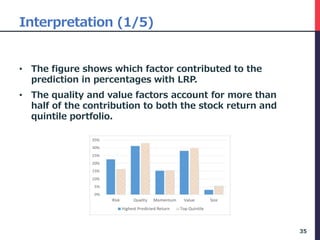
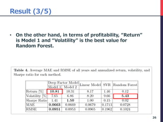
39. Interpretation (5/5)
• In general, the momentum factor is not very
effective, but the value factor is effective in the
Japanese stock markets [Fama2012]
• On the other hand, there is a significant trend in
Japan to evaluate companies that will increase ROE
over the long term.
39

40. Contents
1.Introduction
2.Deep Factor Model
3.Experiment
4.Interpretation of Deep Factor Model
5.Conclusion
40

41. Conclusions
• As a return model, the deep factor model
outperforms the linear model.
• This implies that the relationship between the stock
returns and the factors is nonlinear rather than
linear.
• The shallow model is superior in accuracy, while the
deep model is more profitable.
• Using LRP, it is possible to intuitively determine
which factor contributed to prediction.
41

42. Thank you