This educational file provides complete Solutions for Problems and Exercises from Celestial and Stellar Dynamics by Barbara Ryden. It is designed for students and researchers in astrophysics, astronomy, and theoretical physics who want to strengthen their understanding of stellar motion, orbital mechanics, and galactic dynamics through detailed, structured solutions. Each solution has been carefully prepared to illustrate the mathematical reasoning behind celestial motion, star cluster evolution, and galactic gravitational interactions. The explanations connect fundamental mechanics with advanced astrophysical modeling, making it a valuable study guide for anyone exploring how stars, planets, and galaxies move and interact in space. Key features include: Step-by-step solutions for every exercise and derivation in the text. Clear demonstration of key topics such as two-body and N-body problems, energy conservation, angular momentum, and tidal forces. Detailed treatment of stellar orbits, perturbation theory, resonances, and galactic structure. Integrates Newtonian and modern computational methods for realistic astrophysical systems. Practical application of theory to planetary systems, binary stars, and galactic rotation curves. This collection emphasizes conceptual understanding as much as computational accuracy. Each answer begins with a theoretical overview, followed by mathematical derivation and interpretive discussion, helping learners connect equations to real astrophysical behavior. Students can easily visualize how gravitational interactions shape the structure and evolution of galaxies and star clusters. Useful for: Undergraduate and graduate courses in Celestial Mechanics, Astrophysics, or Stellar Dynamics. Independent learners preparing for exams or research projects. Instructors seeking verified examples and problem references for lectures. By following these detailed solutions, readers will gain confidence in applying mathematical physics to cosmic systems, analyzing orbital stability, and exploring the physical principles behind stellar evolution and galactic motion.

2. 1
Newtonian Dynamics
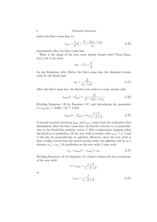
1.1) Approximate the Earth’s orbit relative to the Sun as a circle with a
radius of 1 astronomical unit and an orbital period of 1 sidereal year. Now
imagine that the Sun instantaneously loses a fraction f of its total mass (per-
haps through the meddling of technologically advanced, but ethically dubious,
space aliens).
a) Compute the values of a and e for the Earth’s new orbit around the lower-
mass Sun. [Hint: use the position and velocity of the Earth at the instant of
the Sun’s mass loss as initial conditions.]
The length of the sidereal year is P⊕ ≈ 3.155 815 × 107 s; the length of the
astronomical unit is a⊕ ≈ 1.495 979 × 1013 cm. Thus, the speed of the Earth
on its idealized circular orbit before the Sun’s sudden mass loss is
v⊕ =
2πa⊕
P⊕
≈ 2.978 474 × 106
cm s−1
,
while its specific angular momentum is
j⊕ = a⊕v⊕ ≈ 4.455 733 × 1019
cm2
s−1
.
Immediately after the Sun’s sudden mass loss, the Earth is at a distance r =
a⊕ from the Sun, moving with a speed v⊕ exactly perpendicular to the Sun –
Earth line; thus, the Earth’s specific angular momentum j⊕ is unchanged by
the Sun’s mass loss. However, the standard gravitational parameter of the
Sun – Earth system drops from µold = µ⊙ + µ⊕ to µnew = (1 − f)µ⊙ + µ⊕.
This means that the specific orbital energy increases from (Equation 1.29)
ϵold =
1
2
v2
⊕ −
µ⊙ + µ⊕
a⊕
(1.A)
s
m
t
b
9
8
@
g
m
a
i
l
.
c
o
m
WhatsApp: https://wa.me/message/2H3BV2L5TTSUF1 - Telegram: https://t.me/solutionmanual
You can access complete document on following URL. Contact me if site not loaded
Contact me in order to access the whole complete document - Email: smtb98@gmail.com
https://solumanu.com/product/celestial-and-stellar-dynamics/

3. 2 Newtonian Dynamics
before the Sun’s mass loss, to
ϵnew =
1
2
v2
⊕ −
(1 − f)µ⊙ + µ⊕
a⊕
(1.B)
immediately after the Sun’s mass loss.
What is the shape of the new, more loosely bound orbit? From Equa-
tion 1.43, I can write
a(1 − e2
) =
j2
µ
for any Keplerian orbit. Before the Sun’s mass loss, the idealized circular
orbit for the Earth had
a⊕ =
j2
⊕
µ⊙ + µ⊕
. (1.C)
After the Sun’s mass loss, the Earth’s new orbit is a conic section with
anew(1 − e2
new) =
j2
⊕
(1 − f)µ⊙ + µ⊕
. (1.D)
Dividing Equation 1.D by Equation 1.C, and introducing the parameter
δ ≡ µ⊕/µ⊙ = 3.003 × 10−6, I find
anew(1 − e2
new) = a⊕
1 + δ
1 − f + δ
. (1.E)
A second equation involving anew and enew comes from the realization that
immediately after the Sun’s mass loss, the Earth’s velocity ⃗
v⊕ is perpendic-
ular to the Earth-Sun position vector ⃗
r. This configuration happens when
the Earth is at perihelion. (If the new orbit is bound, with enew < 1, ⃗
v and
⃗
r will also be perpendicular at aphelion. However, since the new orbit is
more weakly bound than the initial circular orbit, the aphelion will be at a
distance rap > a⊕.) At perihelion on the new orbit, I may write
rpe = anew(1 − enew) = a⊕. (1.F)
Dividing Equation 1.E by Equation 1.F, I find a relation for the eccentricity
of the new orbit:
1 + enew =
1 + δ
1 − f + δ
,
or
enew =
f
1 − f + δ
. (1.G)

4. Newtonian Dynamics 3
Substitution into Equation 1.F gives the semimajor axis of the new orbit:
anew = a⊕
1 − f + δ
1 − 2f + δ
.
Note that if the Sun’s mass loss is small (f ≪ 1), the new eccentricity will
be enew ≈ f ≪ 1, and the new semimajor axis will be
anew ≈ (1 + f)a⊕.
b) For what values of f will the Earth’s new orbit be unbound?
For the new orbit to be unbound, with enew ≥ 1, Equation 1.G tells us the
naughty space aliens must remove a fraction f ≥ fmin of the Sun’s mass,
where
fmin =
1 + δ
2
≈ 0.500 0015.
In other words, they must remove at least half the total mass of the Sun –
Earth system.
1.2) Consider a system consisting of two point masses: the primary has mass
m1 and the secondary has mass m2 < m1. The masses are attracted to each
other by a central force F whose amplitude is given by the law
F = Hm1m2r, (1.H)
where H is a constant with units g−1 s−2.
a) Show that the orbit of the secondary relative to the primary is an ellipse
with the primary at the center.
Let the positions of the primary and secondary in an inertial frame of refer-
ence be ⃗
x1 and ⃗
x2 respectively. With the amplitude of the attractive central
force given by Equation 1.H, the equation of motion for the primary is
d2⃗
x1
dt2
= Hm2rr̂,
where the unit vector r̂ points from the primary to the secondary. Similarly,
the equation of motion for the secondary is
d2⃗
x2
dt2
= −Hm1rr̂.
The equation of relative motion, using the coordinate ⃗
r ≡ ⃗
x2 − ⃗
x1 = rr̂, is
then
d2⃗
r
dt2
= −H(m1 + m2)⃗
r. (1.I)

5. 4 Newtonian Dynamics
This equation can also be written in the form
d2⃗
r
dt2
= −
dΦ
dr
r̂,
where the associated potential is
Φ(r) =
1
2
ω2
r2
,
with
ω ≡ [H(m1 + m2)]1/2
having the dimensionality of a frequency.
Since the force is a central force, both the specific energy ϵ = Φ + v2/2
and the specific angular momentum ⃗
ȷ = ⃗
r × ⃗
v are conserved. In the orbital
plane, it is useful to set up a cartesian coordinate system with its origin at
the position of the primary (⃗
r = 0). The cartesian coordinates are useful
because in the two orthogonal directions (call them x and y), the equation
of motion (Eq. 1.I) can be written as
d2x
dt2
= −ω2
x (1.J.x)
d2y
dt2
= −ω2
y, (1.J.y)
Behold! In both the x and y direction, the motion is that of a harmonic
oscillator with frequency ω.
Suppose that at time t = 0, the position of the secondary is (x0, y0) and
the velocity is (vx0, vy0). The solution to Equations 1.J.x and 1.J.y is then
x(t) = x0 cos ωt +
vx0
ω
sin ωt (1.K.x)
y(t) = y0 cos ωt +
vy0
ω
sin ωt. (1.K.y)
Since the oscillation frequency ω is the same in both the x and y directions,
the secondary’s orbit is a closed curve with orbital period P = 2π/ω. That
is, the position of the secondary at time t is the same as its position at times
t + P, t + 2P, t + 3P, and so forth.
How do I show that the closed orbit is an ellipse centered at (x, y) = (0, 0)?
It is not intuitively obvious that Equations 1.K.x and 1.K.y represent an
ellipse. (At least not to my intuition!) However, as frequently happens in
science, we can make the math simpler by choosing the right coordinate
system. Since the secondary is on a closed, bound orbit, at least once per
orbital period P it must reach a maximum distance rap from the primary.

6. Newtonian Dynamics 5
At this maximum distance, since specific energy is conserved, it must have
its minimum speed vap relative to the primary, with
1
2
v2
ap = ϵ −
1
2
ω2
r2
max.
Since rap is a maximum in r, the velocity ⃗
vap must be perpendicular to
⃗
rap. I now cunningly choose my initial time (t = 0) to be an instant when
r = rap. I orient my cartesian coordinates so that (x0, y0) = (rap, 0) and
(vx0, vy0) = (0, vmin). Using this set of coordinates, Equations 1.K.x and
1.K.y simplify to
x(t) = rap cos ωt (1.L.x)
y(t) =
vap
ω
sin ωt. (1.L.y)
Thus, in these coordinates, I can write
x(t)2
r2
ap
+
y(t)2
v2
ap/ω2
= cos2
ωt + sin2
ωt = 1,
which is the equation for an ellipse whose axes correspond to the x and y
axis. The semimajor axis of the ellipse is a = rap and the semiminor axis is
b = vap/ω.
b) What is the dependence of the secondary’s orbital period P on the semi-
major axis a of its orbit?
Since the orbital period is P = 2π/ω, and ω depends only on the total mass
m1 + m2 and the constant H, the orbital period P is independent of the
semimajor axis a.
1.3) Consider a different system consisting of two point masses with m1 >
m2. These masses are attracted to each other by a central force F whose
amplitude is given by the inverse cube law
F =
Km1m2
r3
, (1.M)
where K is a constant with units cm4 g−1 s−2. This potential does not, in
general, have a neat analytic form for orbital shapes. However, we can look
at limiting cases.
a) Suppose the point masses start at rest relative to each other, with a sep-
aration r. How long will it be until the attractive force causes the masses to
meet? [Hint: a numerical solution of a differential equation may be useful
here.]

7. 6 Newtonian Dynamics
Let the positions of the primary and secondary in an inertial frame of refer-
ence be ⃗
x1 and ⃗
x2 respectively. With the amplitude of the attractive central
force given by Equation 1.M, the equation of motion for the primary is
d2⃗
x1
dt2
= Km2r3
r̂,
where the unit vector r̂ points from the primary to the secondary. Similarly,
the equation of motion for the secondary is
d2⃗
x2
dt2
= −Km1r3
r̂.
The equation of relative motion, using the coordinate ⃗
r ≡ ⃗
x2 − ⃗
x1 = rr̂, is
then
d2⃗
r
dt2
= −K(m1 + m2)r3
r̂. (1.N)
For purely radial motion, this reduces to
d2r
dt2
= −K(m1 + m2)r3
. (1.O)
If I begin with initial conditions r = r0, v = 0, the initial acceleration, from
Equation 1.O, will be
a0 =
K(m1 + m2)
r3
0
.
Thus, the relevant time scale for the infall will be
t0 ≡
r2
0
a0
1/2
=
r2
0
[K(m1 + m2)]1/2
.
Using the dimensionless time τ ≡ t/t0 and the dimensionless radius ρ ≡ r/r0,
the dimensionless equation of radial relative motion is
d2ρ
dτ2
= −
1
ρ3
, (1.P)
with initial conditions ρ = 1 and dρ/dτ = 0. As you can verify by substitu-
tion, the appropriate solution to Equation 1.P is
ρ(τ) = (1 − τ2
)1/2
,
implying that the time elapsed until ρ = r = 0 is τ = 1, or
t = t0 =
r2
0
[K(m1 + m2)]1/2
.
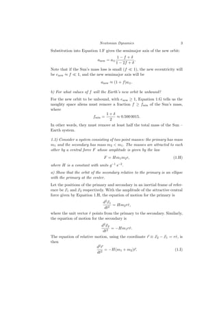
b) Consider the special case where the relative orbit of the masses is a perfect

8. Newtonian Dynamics 7
circle with radius r. What is the dependence of the orbital period P on the
orbital radius r?
The acceleration of the secondary relative to the primary is (Equation 1.N)
d2⃗
r
dt2
= −K(m1 + m2)r3
.
For this acceleration to match the required centripetal acceleration for a
circular orbit,
d2⃗
r
dt2
= −
v2
r
= −
2πr
P
2
1
r
,
we need
K(m1 + m2)r3
=
4π2r
P2
,
or
P = 2π
r2
[K(m1 + m2)]1/2
.
To generalize, if the attractive force has the dependence F ∝ r−n, the re-
lation between orbital period and orbital radius will be P ∝ r(1+n)/2 for a
circular orbit.