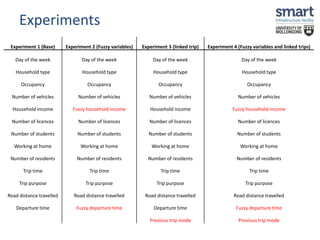
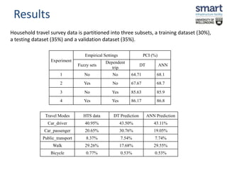
This document discusses a study on estimating travel mode choices using data mining and fuzzy techniques, focusing on household trips in Sydney. It details the methodology involving artificial neural networks and decision trees, incorporating fuzzy sets for certain variables to enhance predictive accuracy. The results indicate that incorporating fuzzy and tour-based models outperforms traditional crisp data approaches in predicting travel modes.

1. Tour-based Travel Mode Choice Estimation
based on
Data Mining and Fuzzy Techniques
Nagesh Shukla, Jun Ma, Rohan Wickramasuriya, Nam Huynh, Pascal Perez
Presented by:
Pascal Perez
Research Director
perez@uow.edu.au

2. Classification of literature in mode choice
Data
Type
Trip Type
Discrete Choice Models Machine Learning
Crisp Data Crisp & Fuzzy Data Crisp Data
Crisp &
Fuzzy
Data
Independent Trips
Gaudry, (1980);
McFadden (1973);
Daly & Zachary
(1979); Hensher &
Ton (2000)
Dell'Orco et al.
(2007)
Xie et al. 2003;
Reggiani & Tritapepe
1998; Cantarella et al.,
2003; Shmueli et al.
1996; Edara 2003;
Hensher and Ton, 2000
Yaldi, G.
(2005)
Linked Individual
Trips (tour-based)
Miller et al. (2005) - Biagioni et al., (2008) This Study
Linked Household
Trips
Miller et al. (2005) - Future Work
Future
Work

3. Machine learning methods
Input Layer Hidden Layer Output Layer
Back-propagation algorithms for ANN training
- Scaled conjugate gradient (Moller 1993)
-Levenberg-Marquardt optimization (Hagan and
Menhaj, 1994)
(http://iasri.res.in/ebook/win_school_aa/notes/Decision_tree.pdf)
Decision trees
- are easy to assimilate by humans thanks to their
intuitive representation
- do not require too much parameter settings
- can be constructed fairly fast and its accuracy is
comparable to other classification models.
DT algorithms such as C4.5 and Classification and
Regression Technique (CART) have been identified as
top 10 data mining algorithms in terms of its wider
applicability.

4. Case study - HTS data for Sydney GMA
• 3000-3500 household participants each
year. Dataset covers 5 years.
• 14 variables include
– Day of the week
– Household type
– Occupancy
– Number of vehicles
– Household income
– Number of people holding a valid licence
– Number of students
– Working at home
– Total number of residents
– Trip time *
– Trip purpose
– Road distance travelled
– Departure time *
– Travel mode
(http://www.bts.nsw.gov.au/Images/UserUploadedImages/86/hts-gma-map.jpg)

5. Data pre-processing
• Linking consecutive trips of an individual
Let (X,Y) be a survey dataset of trips made by L travellers, where (xlm,ylm)
collectively represents information of the mth trip made by the traveller l, m Є {1,
2, ..., Ml}, l Є {1, 2, ..., L}.
is a collection of explanatory variables and ylm is the travel
mode of the mth trip made by the traveller l.
To account for impact of consecutive trips, a new explanatory variable
representing the mode of the previous trip is defined as
,

6. Data preprocessing (cont.)
• Fuzzifying explanatory variables departure time
Four fuzzy sets of departure are defined, “2 hour am peak (7-9am), 6 hour inter-peak
(9am-3pm), 3 hour evening peak (3-6pm) and the remaining evening/night period”
(Sydney Strategic Travel Model – Modelling future travel patterns, February 2011 Release, Technical Documentation)

7. Data preprocessing (cont.)
• Fuzzifying explanatory variables household income
Low income: “Persons in the
second and third income
deciles”
Middle income: “Persons in the
middle income quintile”
High income: “Persons in the
top income quintile”
(Australian Bureau of Statistics – Household Income
and Income Distribution, 6523.0, 2011-2012)
Household income in survey data, ranging from AU$5006 to AU$402741, is classified
into three fuzzy sets ‘low income’, ‘middle income’, and ‘high income’.

8. Experiments
Experiment 1 (Base) Experiment 2 (Fuzzy variables) Experiment 3 (linked trip) Experiment 4 (Fuzzy variables and linked trips)
Day of the week Day of the week Day of the week Day of the week
Household type Household type Household type Household type
Occupancy Occupancy Occupancy Occupancy
Number of vehicles Number of vehicles Number of vehicles Number of vehicles
Household income Fuzzy household income Household income Fuzzy household income
Number of licences Number of licences Number of licences Number of licences
Number of students Number of students Number of students Number of students
Working at home Working at home Working at home Working at home
Number of residents Number of residents Number of residents Number of residents
Trip time Trip time Trip time Trip time
Trip purpose Trip purpose Trip purpose Trip purpose
Road distance travelled Road distance travelled Road distance travelled Road distance travelled
Departure time Fuzzy departure time Departure time Fuzzy departure time
Previous trip mode Previous trip mode

9. Results
Household travel survey data is partitioned into three subsets, a training dataset (30%),
a testing dataset (35%) and a validation dataset (35%).
Experiment
Empirical Settings PCI (%)
Fuzzy sets
Dependent
trip
DT ANN
1 No No 64.71 68.1
2 Yes No 67.67 68.7
3 No Yes 85.63 85.9
4 Yes Yes 86.17 86.8
Travel Modes HTS data DT Prediction ANN Prediction
Car_driver 40.95% 43.50% 43.11%
Car_passenger 20.65% 30.76% 19.05%
Public_transport 8.37% 7.54% 7.74%
Walk 29.26% 17.68% 29.55%
Bicycle 0.77% 0.53% 0.53%

10. Conclusions
• New methodology for travel mode choice using artificial
neural network and decision trees.
• The methodology considers
– Expert judgements by using fuzzy sets instead of crisp data for some
explanatory variables.
– Tour based model that accounts for the dependency of modes
between trips
• Travel mode prediction using fuzzified explanatory variables
combined with tour based model proved to out-perform
predictions using crisp variables.
• Future work could involve more explanatory variables, new
fuzzy sets, and account for dependencies between trips of
individuals in the same household.

11. Questions