BasicGraphsWithR

by
Aureliano Bombarely Gomez
Boyce Thompson Institute for Plant
Research
Tower Road
Ithaca, New York 14853-1801
U.S.A.
Graphs With R

Graphs with R:
1. Introduction to R
1.1. R Software and documentation
1.2. Basic R variables
2. Gallery of R Graphs and Popular Packages
2.1. Basic graphs
2.2. Gplots and ggplot2 (expanding graphs)
2.3. Corrplot (correlation matrices)
2.4. Ape (phylogenies)
3. Steps and Functions.
4. Examples

1. Introduction to R
R is a language and environment for statistical
computing and graphics..

1.1 R Software and documentation
https://www.rstudio.com/
RStudio IDE is a powerful and productive user interface for R.
R STUDIO:

1 - Menu
2 - File viewer
3 - Console
4a - Variable list
4b - History
5a - File browser
5b - Plots
5c - Packages
5d - Manuals

WEB:
OFICIAL WEB: http://www.r-project.org/index.html
QUICK-R: http://www.statmethods.net/index.html
BOOKS:
• Introductory Statistics with R (Statistics and Computing), P.
Dalgaard [available as manual at R project web]
• The R Book, MJ. Crawley
R itself: help() and example()

Basic RVariables:
★ Vectors.
★ Matrices and arrays.
★ Dataframes and list.
1.2 Basic R variables

Basic RVariables:
★ Vectors.
Most simple 'data structure' in R. Ordered collection
of data values.
To create a vector use command: c()
Examples:
count = c(1, 2, 3, 4, 5, 6)
plants = c(“tomato”, “potato”, “soybean”)

Basic RVariables:
★ Vectors.
Operation with vectors:
• Addition: x + y
• Substraction: x - y
• Division: x / y
• Exponentation: x ^ y
• Square root: sqrt(x)
• Absolute value: abs(x)
• Mean and median: mean(x) and median(x).

Basic RVariables:
A matrix is a two dimension vector with positive values.
To create a matrix use command: matrix(c(), ncol, nrow)
Examples:
mtx1 = matrix(c(1, 4, 8, 9, 5, 6, 2, 1, 1), ncol=3, nrow=3)
1 4 8
9 5 6
2 1 1

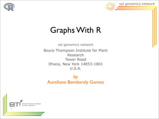
Basic RVariables:
Matrices have index and they can be replaced by
names
[ ,1] [ ,2] [ ,3]
[1, ] 1 4 8
[2, ] 9 5 6
[3, ] 2 1 1
mtx1[1,3] 8
mtx1[2,] c(9,5,6)

Basic RVariables:
An array is a vector with N dimensions
To create an array use command: array(c(), dim=c())
Examples:
array1 = matrix(c(1, 4, 8, 9, 5, 6, 2, 1), dim=c(2,2,2))
1 4
8 9
5 6
2 1

Basic RVariables:
Arrays also have indexes
array1[1,2,1] 4
array1[2,2] c(9,1)
1 4
8 9
5 6
2 1
array1[2,] matrix(1,4,8,9)

Basic RVariables:
★ List and dataframes.
A list is an object object consisting of an ordered collection of
other objects as its components
Example:
test = list(c(1, 4, 8, 9, 5, 6, 2, 1), c(“red”, “blue”), mtx1)
To create a list use command: list()

Basic RVariables:
A dataframe is a list con 4 specific features:
To create a data frame use command: data.frame()
1.The components must be vectors (numeric, character, or logical), factors,
numeric matrices, lists, or other data frames.
2.Matrices, lists, and data frames provide as many variables to the new data frame
as they have columns, elements, or variables, respectively.
3.Numeric vectors, logicals and factors are included as is, and character vectors are
coerced to be factors, whose levels are the unique values appearing in the vector.
4.Vector structures appearing as variables of the data frame must all have the
same length, and matrix structures must all have the same row size.

Basic RVariables:
A dataframe can be imported/exported to/from R using:
read.table(file)
write.table(data.frame, file)

Graphs are R functions that produce a graphical output.
R functions: Objects with a set of instructions to process
some data or to produce a graphical output.
name(arguments)

library("maps")
http://rgraphgallery.blogspot.com/

Depends of the package:
+ Basic package functions:
plot() simple plots
hist() density plots
dotchart() simple dotplots
barplot() simple bar graphs
pie() simple pie graphs
boxplot() boxplot graphs
2.1 Basic Graphs

2.1 Basic Graphs
Data for these examples: http://data.kew.org/cvalues/ Solanaceae
file: data001_genome_size.csv

0 20 40 60 80 100
0500010000150002000025000
Genome Size for Solanaceae
chromosome number
genomesize(Mb)
plot() simple plots
2.1 Basic Graphs
plot(plant_genome_sizes$chromosome_number, plant_genome_sizes$genome_size, pch=19, xlab="chromosome number",
ylab="genome size (Mb)", xlim=c(0,100), main="Genome Size for Solanaceae")

Histogram for Solanaceae Plant Genome Size
genome size
Frequency
0 5000 10000 15000 20000 25000
05101520253035
hist() density plots
2.1 Basic Graphs
hist(plant_genome_sizes$genome_size, breaks=c(100), col=c("black"), xlab="genome size", main="Histogram for
Solanaceae Plant Genome Size")

parviflora
inflata
violacea
altiplana
integrifolia
occidentalis
axillaris
reitzii
saxicola
bonjardinensis
kleinii
scheideana
helianthemoides
variabilis
pubescens
alpicola
bajeensis
interior
littoralis
riograndensis
parodii
guarapuavensis
mantiqueirensis
exserta
hybrida
500 1000 1500 2000
Petunia species genome size
Genome Size (Mb)
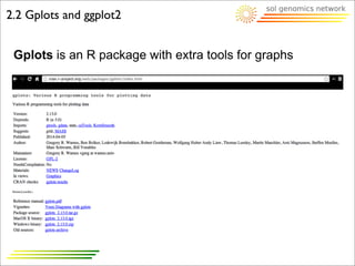
dotchart() simple dotplots
2.1 Basic Graphs
petunia_sizes = plant_genome_sizes[plant_genome_sizes$genus == "Petunia",]
dotchart(petunia_sizes$genome_size, labels=petunia_sizes$species, xlab="Genome Size (Mb)", xlim=c(500,2000),
main="Petunia species genome size")

Atropa
Calibrachoa
Capsicum
Cyphomandra
Datura
Hyoscyamus
Lycium
Lycopersicon
Nicotiana
Petunia
Solanum
Withania
Solanaceae genome sizes by Genus
0
2000
4000
6000
8000
10000
barplot() simple bar graphs
2.1 Basic Graphs
genome_size_by_genus = aggregate(plant_genome_sizes$genome_size, by=list(plant_genome_sizes$genus), FUN=mean)
barplot(genome_size_by_genus$x, names.arg=genome_size_by_genus$Group.1, las=2, cex.names=0.5, col="black",
main="Solanaceae genome sizes by Genus")

Atropa
Calibrachoa
Capsicum
Cyphomandra
Datura
Hyoscyamus
Lycium
Lycopersicon
Nicotiana
Petunia
Solanum
Withania
Species Percentage by Genus
pie() simple pie graphs
2.1 Basic Graphs
species_count = table(plant_genome_sizes$genus)
pie(species_count, radius=1, init.angle=90, col=rainbow(12), main="Species Percentage by Genus")

Atropa
Calibrachoa
Capsicum
Cyphomandra
Datura
Hyoscyamus
Lycium
Lycopersicon
Nicotiana
Petunia
Solanum
Withania
0
5000
10000
15000
20000
25000
Genome Size distribution by Genus
boxplot() boxplot graphs
2.1 Basic Graphs
by_genus = split(plant_genome_sizes$genome_size, plant_genome_sizes$genus)
boxplot(by_genus, las=2, main="Genome Size distribution by Genus", col=c("red", "green", "green", "green", "green", "blue",
"blue", "green", "blue", "green", "red", "blue"), cex.axis=0.6)

2.2 Gplots and ggplot2
Gplots is an R package with extra tools for graphs

Atropa
Calibrachoa
Capsicum
Cyphomandra
Datura
Hyoscyamus
Lycium
Lycopersicon
Nicotiana
Petunia
Solanum
Withania
0
5000
10000
15000
20000
25000
n=1 n=18 n=12 n=11 n=4 n=3 n=4 n=9 n=55 n=25 n=39 n=1
Gplots is an R package with extra tools for graphs:
• balloonplot()
• bandplot()
• barplot2() and boxplot2()
• hist2d()
• overplot()
...
boxplot2(by_genus, las=2, main="Genome Size distribution by Genus",
col=c("red", "green", "green", "green", "green", "blue", "blue", "green",
"blue", "green", "red", "blue"), cex.axis=0.6, top=T)

Gplots is an R package with extra tools for graphs:
• balloonplot()
• bandplot()
• barplot2() and boxplot2()
• hist2d()
• overplot()
...
genome_size_by_genus_sd = aggregate(plant_genome_sizes
$genome_size, by=list(plant_genome_sizes$genus), FUN=sd)
barplot2(genome_size_by_genus$x, names.arg=genome_size_by_genus
$Group.1, las=2, cex.names=0.5, col="black", main="Solanaceae genome
sizes by Genus", ci.l=genome_size_by_genus$x -
genome_size_by_genus_sd$x, ci.u=genome_size_by_genus$x +
genome_size_by_genus_sd$x, plot.ci=T, ylim=c(0,20000))
Atropa
Calibrachoa
Capsicum
Cyphomandra
Datura
Hyoscyamus
Lycium
Lycopersicon
Nicotiana
Petunia
Solanum
Withania
Solanaceae genome sizes by Genus
0
5000
10000
15000
20000

Ggplot2 is an R package with grammar tools for graphs

0e+00
2e−04
4e−04
6e−04
0 5000 10000 15000 20000 25000
genome size
density
poly
Diploid
Tetraploid
Hexaploid
Genome Size density for Solanaceae
Ggplot2 is an R package with grammar tools for graphs
plant_genome_sizes$poly = factor(plant_genome_sizes$polyploidy,
levels=c(2,4,6), labels=c("Diploid", "Tetraploid", "Hexaploid"))
qplot(plant_genome_sizes$genome_size, data=plant_genome_sizes,
geom="density", main="Genome Size density for Solanaceae", fill=poly,
alpha=I(.5), xlab="genome size")

2.3 Corrplot
corrplot is an R package for visualization of correlation
matrix

2.4 Ape
ape is an R package for analysis of phylogenetic and
evolution
http://www.r-phylo.org/wiki/Main_Page

2.4 Ape
phylog is an R package for tree manipulation

Graphical procedures step by step:
1) Enable Graphical Device
(X11/QuartzWindows/ by default)
2) Global graphical parameters for the graphical device
3) High level plot function
4) Low level plot function
3. Steps and functions

Graphical procedures step by step:
1) Enable Graphical Device
bmp(), tiff(), jpeg(), png(), postscript(), pdf().
par()
3) High level plot function
plot(), hist(), dotchart(), barplot(), pie()...
legend(), points(), axis(), text(), mtext()...

par()
Text and
Symbol Size
Plotting
Symbols
Lines Colors
Fonts
Margins and
Graph Size
http://www.statmethods.net/advgraphs/parameters.html

par()
Margins and Graph Size
http://rgraphics.limnology.wisc.edu/rmargins_sf.php
Margins:
par(mar=c(b,l,t,r))
Outer margins:
par(omar=c(b,l,t,r))
b = bottom
l = left
t = top
r = right

par()
Multiple graphs
http://rgraphics.limnology.wisc.edu/rmargins_mfcol.php
Multiple plots:
par(mfcol=(x,y))
x = x_columns
y = y_rows

legend(), points(), axis(), text(), mtext()...
http://www.statmethods.net/advgraphs/axes.html
Titles
Text
Annotations
Axes Legend
Reference
Lines
Points
Atropa
Calibrachoa
Capsicum
Cyphomandra
Datura
Hyoscyamus
Lycium
Lycopersicon
Nicotiana
Petunia
Solanum
Withania
0
5000
10000
15000
20000
25000

Atropa
Calibrachoa
Capsicum
Cyphomandra
Datura
Hyoscyamus
Lycium
Lycopersicon
Nicotiana
Petunia
Solanum
Withania
0
5000
10000
15000
20000
25000
Only Diploids
Diploids and Tetraploids
From Diploids to Hexaploids
legend()
Atropa
Calibrachoa
Capsicum
Cyphomandra
Datura
Hyoscyamus
Lycium
Lycopersicon
Nicotiana
Petunia
Solanum
Withania
0
5000
10000
15000
20000
25000
legend(8,23000, legend=c("Only
Diploids", "Diploids and Tetraploids",
"From Diploids to Hexaploids"),
fill=c("green", "blue", "red"))

NbC25469554g0001
NbC25730842g0001
NbC26298068g0003
NbS00000194g0006
NbS00000341g0006
NbS00000565g0004
NbS00001525g0108
NbS00001801g0009
NbS00002670g0014
NbS00002765g0028
Gene Expression
0
2
4
6
8
10
12
14
EV10
EV21
TS10
TS21
Example I: Gene expression
File: data002_gene_expression.tab
4. Examples

>data002_gene_expression <= read.delim("~/
Desktop/R_Class_Exercises/
data002_gene_expression.tab")
>gene_exp =
as.matrix(data002_gene_expression[,2:5])
4. Examples
0) Data load and preparation
data.frame
matrix

>gene_exp =
>barplot(gene_exp)
4. Examples
1) first plot
Problem:
Grouped by conditions, no by gene.

>gene_exp =
>barplot(t(gene_exp))
4. Examples
1) first plot
Problem:
Grouped by conditions, no by gene.
Solution:
transpose the matrix with t()

>gene_exp =
>barplot(t(gene_exp))
4. Examples
2) second plot
Problem:
Gene expression is stack.

Problem:
Gene expression is stack.
>gene_exp =
>barplot(t(gene_exp), beside=T)
4. Examples
Solution:
use beside=T argument in the
barplot() function
2) second plot

>gene_exp =
4. Examples
3) third plot
Problem:
Wrong limits for the y axis.

Problem:
Wrong limits for the y axis.
>gene_exp =
>barplot(t(gene_exp), beside=T, ylim=c(0,15))
4. Examples
Solution:
use ylim=c(0,15) argument in the
barplot() function
3) third plot

>gene_exp =
4. Examples
4) forth plot
Problem:
No labels for any axis.

Problem:
No labels for any axis.
>gene_exp =
>barplot(t(gene_exp), beside=T, ylim=c(0,15),
ylab="Expression (FPKM)",
names.arg=data002_gene_expression
$gene_short_name, xlab="Gene Name")
4. Examples
Solution:
use ylab=”Expression (FPKM)”,
names.arg=data002_gene_express
ion$gene_short_name and
xlab=”Gene Names”, arguments in
the barplot() function
4) forth plot

>gene_exp =
$gene_short_name, xlab="Gene Name")
4. Examples
5) fifth plot
Problem:
Names in the x axis are too big.

Problem:
Names in the x axis are too big.
>gene_exp =
$gene_short_name, xlab="Gene Name",
las=2)
4. Examples
Solution:
use las=2, argument in the barplot()
function
5) fifth plot

>gene_exp =
las=2)
4. Examples
6) sixth plot
Problem:
Names are incomplete (margin).

Problem:
Names are incomplete (margin).
>gene_exp =
>par(oma=c(8,0,0,0))
las=2)
4. Examples
Solution:
change margins with
par(oma=c(8,0,0,0)
6) sixth plot

>gene_exp =
>par(oma=c(8,0,0,0))
las=2)
4. Examples
7) seventh plot
Problem:
Gene name label is missplaced.

Problem:
Gene name label is missplaced.
>gene_exp =
>par(oma=c(8,0,0,0))
$gene_short_name, las=2)
>mtext("Gene Name", 1, 10)
4. Examples
Solution:
Don’t use xlab= argument. Use
mtext() function instead placing the
label in the outer margin
7) seventh plot

>gene_exp =
>par(oma=c(8,0,0,0))
$gene_short_name, las=2)
4. Examples
8) eighth plot
Problem:
No colors, no title

Problem:
No colors, no title
>gene_exp =
>par(oma=c(8,0,0,0))
$gene_short_name, las=2, col=c("green",
"lightgreen", "blue", "lightblue"), main="Gene
Expression for TS treatment")
4. Examples
Solution:
use col= and main= arguments to
set up a color and a title
8) eighth plot

>gene_exp =
>par(oma=c(8,0,0,0))
4. Examples
9) ninth plot
Problem:
No legend

Problem:
No legend
>gene_exp =
>par(oma=c(8,0,0,0))
>legend(40,13,legend=c("EV10", "EV21",
"TS10", "TS21"), fill=c("green", "lightgreen",
"blue", "lightblue"))
4. Examples
Solution:
use legend() function
9) ninth plot

>gene_exp =
>par(oma=c(8,0,0,0))
4. Examples
10) tenth plot

1) ENABLE GRAPHICAL DEVICE
2) GLOBAL GRAPHICAL PARAMS.
3) HIGH-LEVEL PLOTTING COMMAND
4) LOW-LEVEL PLOTTING COMMAND
4. Examples
>gene_exp =
## Default graphical device
>par(oma=c(8,0,0,0))

Example II:Multiple graphs
File: data001_genome_size.csv
4. Examples

>par(oma=c(2,2,0,0), mar=c(6,5,6,2))
>layout(matrix(c(1,2,3,3), 2, 2, byrow = TRUE))
>plant_genome_sizes <- read.delim("~/Desktop/R_Class_Exercises/data001_genome_size.csv")
>genome_size_by_genus = aggregate(plant_genome_sizes$genome_size, by=list(plant_genome_sizes$genus),
FUN=mean)
>barplot(genome_size_by_genus$x, names.arg=genome_size_by_genus$Group.1, las=2, cex.names=1,
col="black", main="Solanaceae genome sizes by Genus")
>mtext("Genome Size (Mb)", 2, 4)
species_count = table(plant_genome_sizes$genus)
>pie(species_count, radius=1, init.angle=90, col=rainbow(12), main="Species Percentage by Genus")
>library("gplots")
>by_genus = split(plant_genome_sizes$genome_size, plant_genome_sizes$genus)
>boxplot2(by_genus, las=2, main="Genome Size distribution by Genus", col=c("red", "green", "green", "green",
"green", "blue", "blue", "green", "blue", "green", "red", "blue"), cex.axis=1, top=T)
>legend(8,23000, legend=c("Only Diploids", "Diploids and Tetraploids", "From Diploids to Hexaploids"),
fill=c("green", "blue", "red"))
>mtext("Genome Size (Mb)", 2, 4)
Example II:Multiple graphs
File: data001_genome_size.csv
4. Examples

BasicGraphsWithR

More Related Content

What's hot

Viewers also liked

Similar to BasicGraphsWithR

Recently uploaded

BasicGraphsWithR