Downloaded 617 times


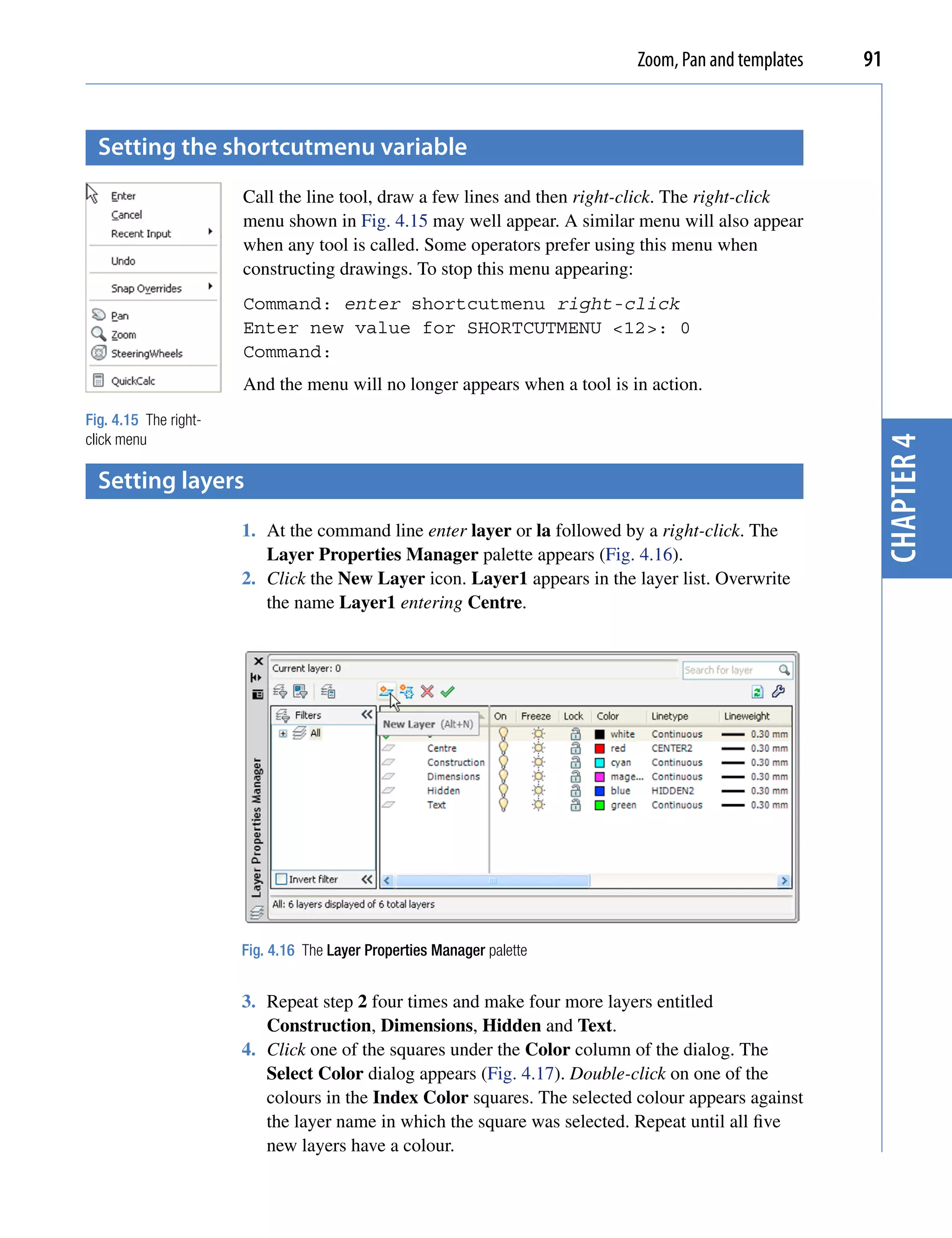
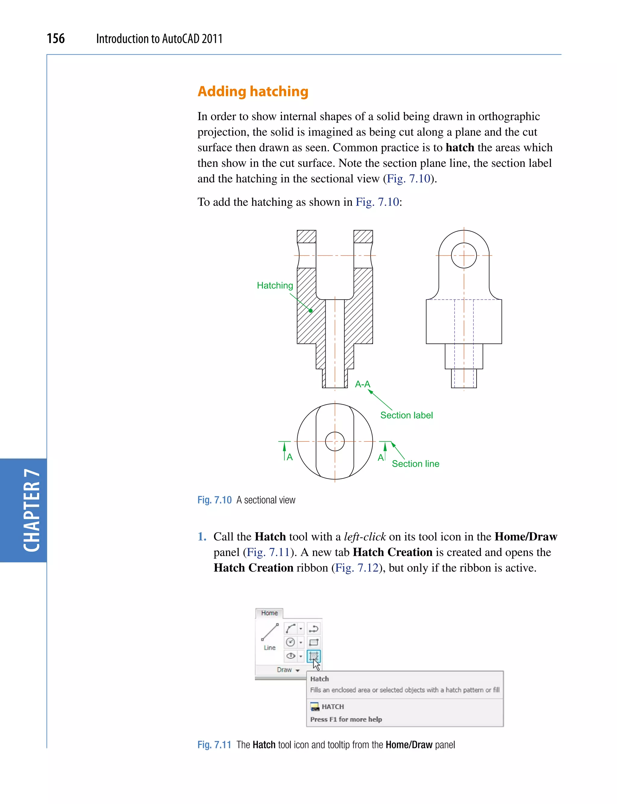
![20 Introduction to AutoCAD 2011
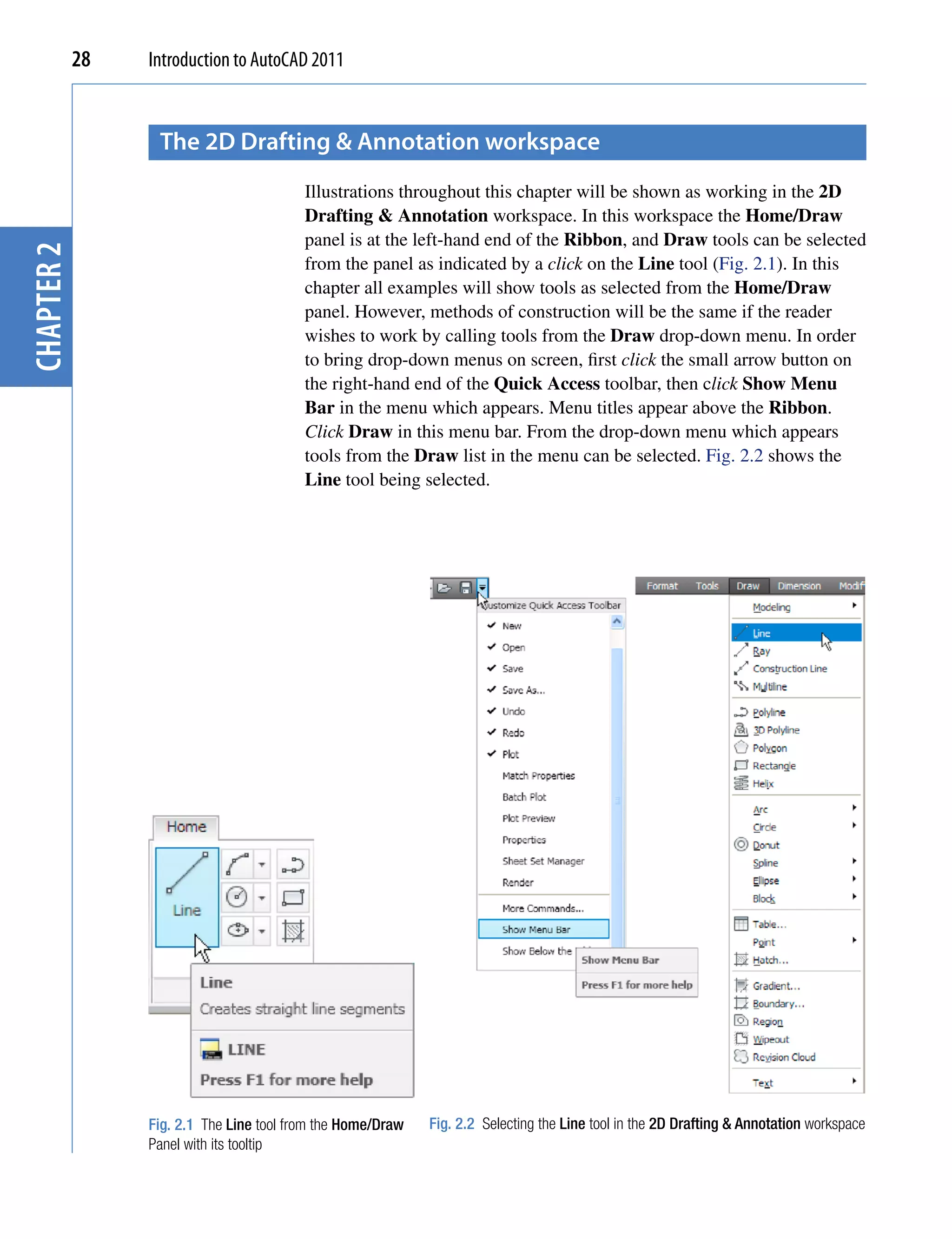
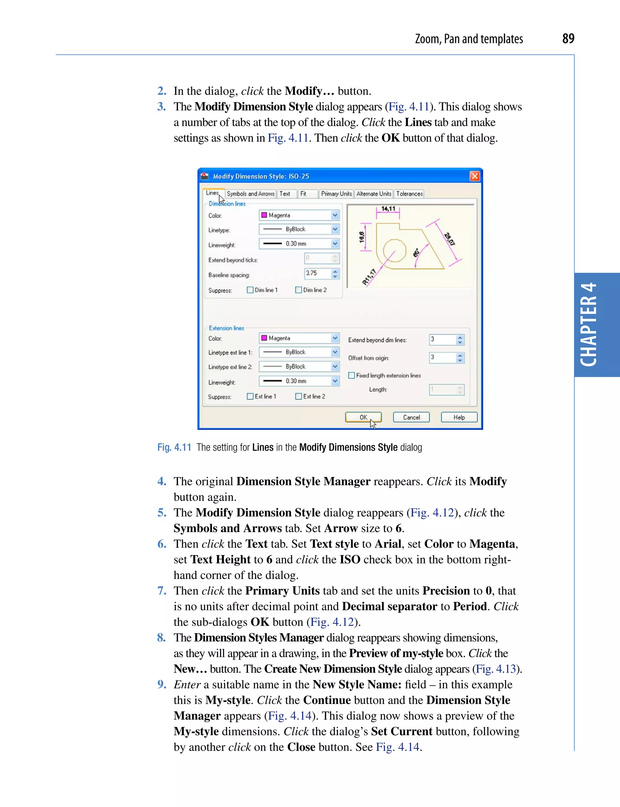
Methods of showing entries in the command palette
CHAPTER 1
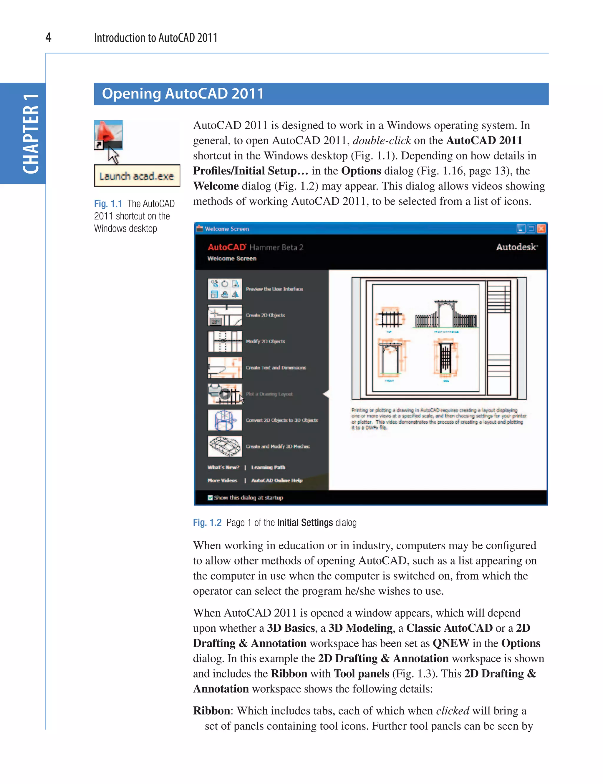
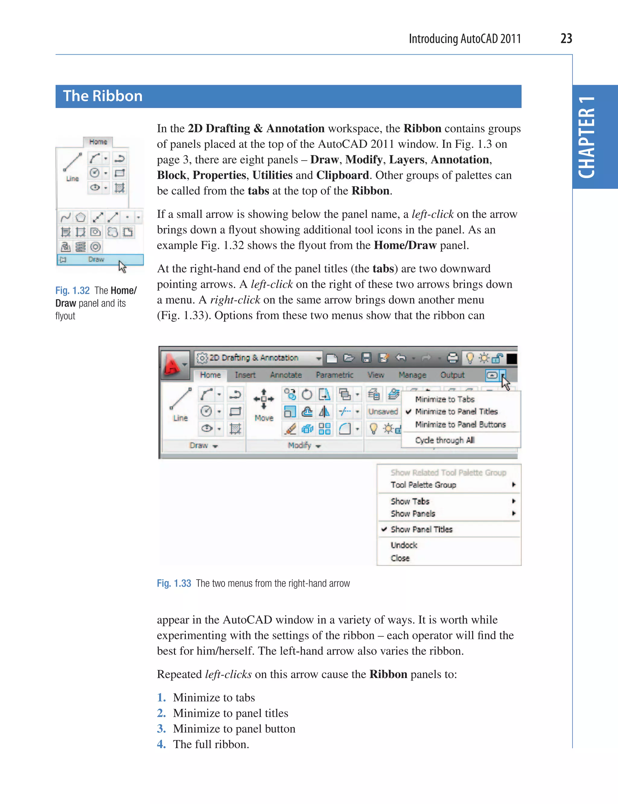
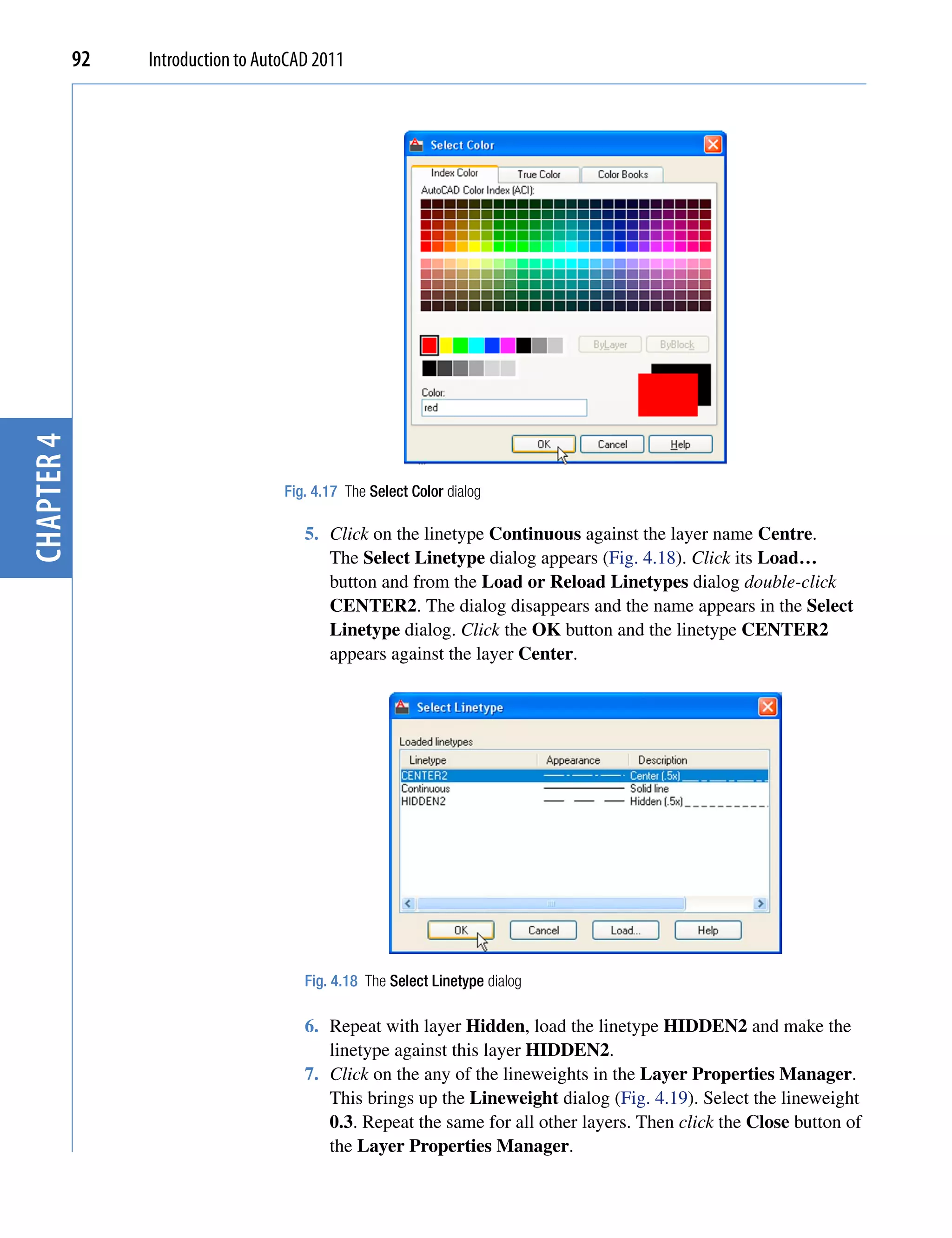
Throughout the book, a tool is “called” usually by a click on a tool icon
in a panel – in this example entering zoom at the command line and the
following appears in the command palette:
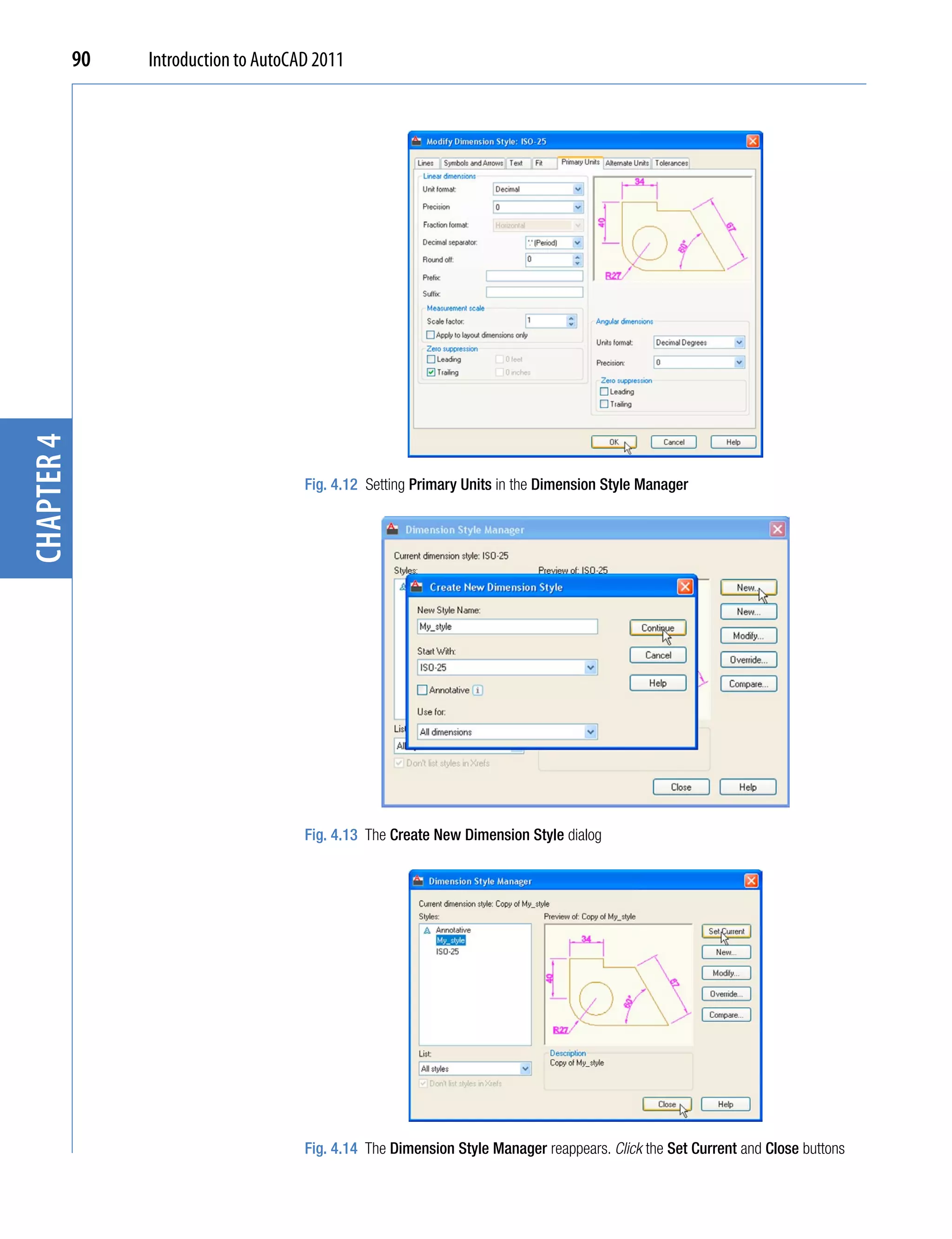
Command: enter zoom right-click
Specify corner of window, enter a scale factor
(nX or nXP), or [All/Center/Dynamic/Extents/
Previous/Scale/Window/Object] <real time>: pick
a point on screen
Specify opposite corner: pick another point to
form a window
Command:
Note
In later examples this may be shortened to:
Command: zoom
[prompts]: following by picking points
Command:
Notes
1. In the above enter means type the given letter, word or words at the
Command: prompt.
2. Right-click means press the Return (right) button of the mouse or
press the Return key of the keyboard.
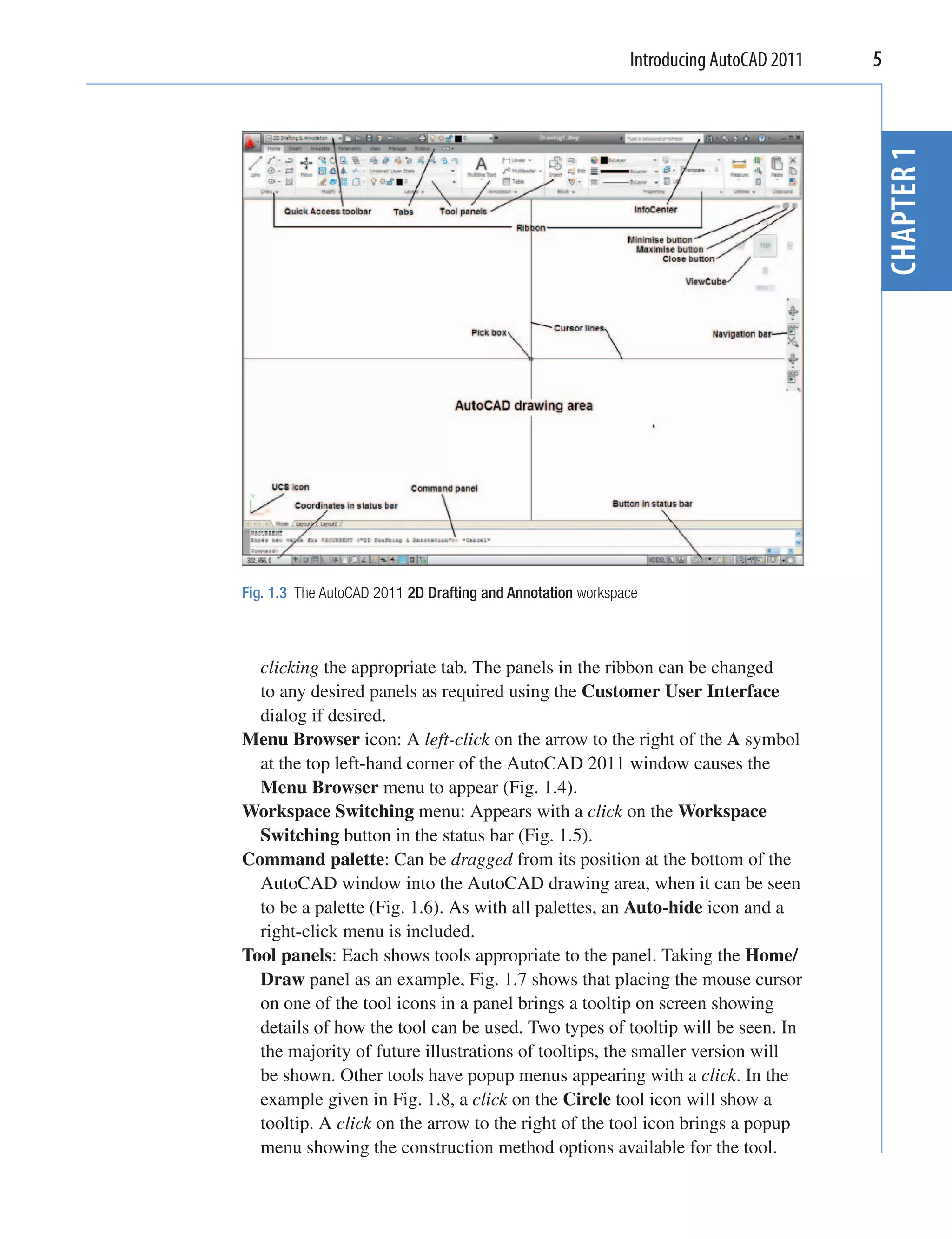
Tools and tool icons
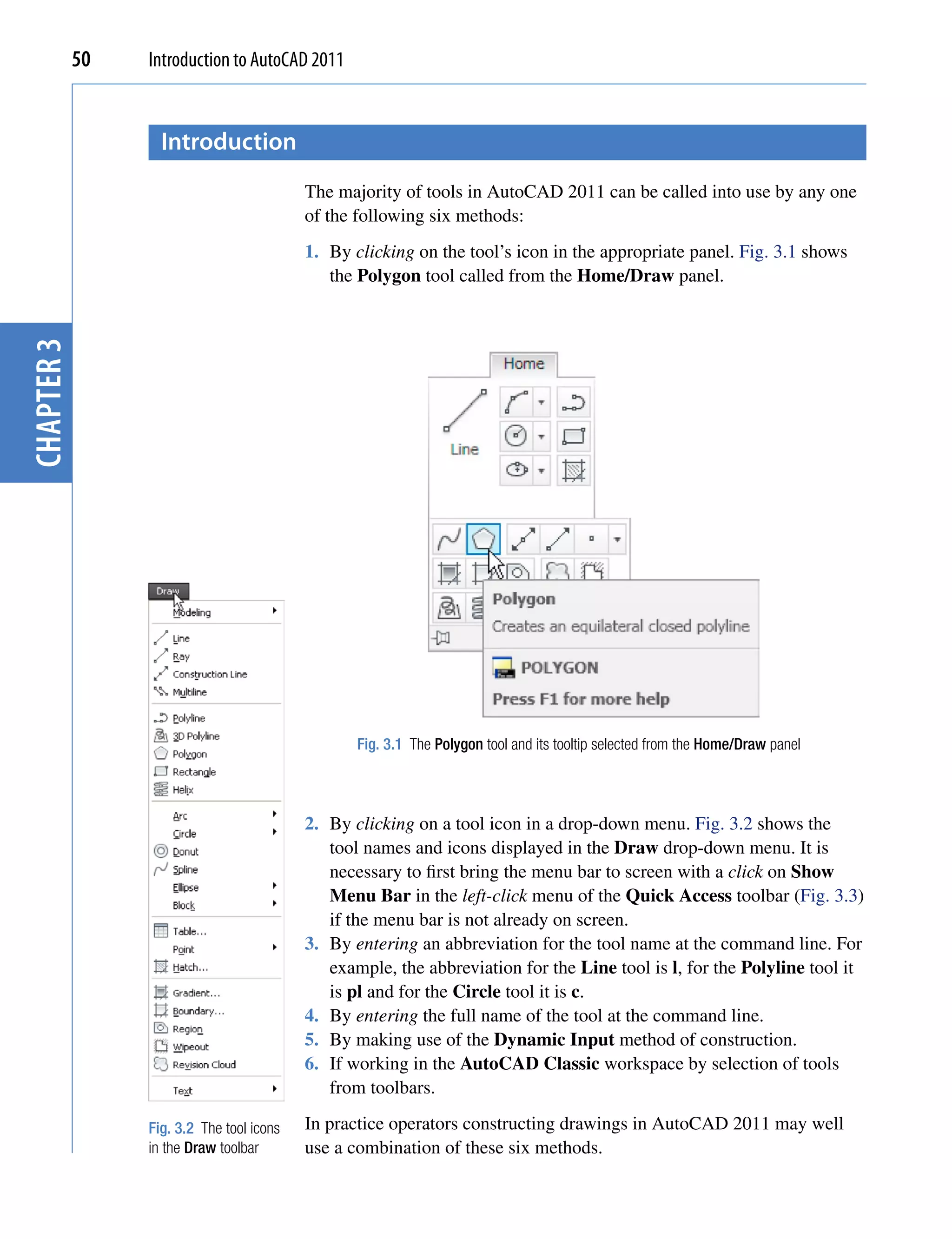
In AutoCAD 2011, tools are shown as names and icons in panels or in
drop-down menus. When the cursor is placed over a tool icon a description
shows with the name of the tool as shown and an explanation in diagram
form as in the example given in Fig. 1.7 (page 5).
If a small outward-facing arrow is included at the right-hand side of a tool
icon, when the cursor is placed over the icon and the pick button of the
mouse depressed and held, a flyout appears which includes other features.
An example is given in Fig. 1.8 (page 5).](https://image.slidesharecdn.com/introductiontoautocad2011-100614022653-phpapp02/75/Introduction-to-AutoCad-2011-19-2048.jpg)

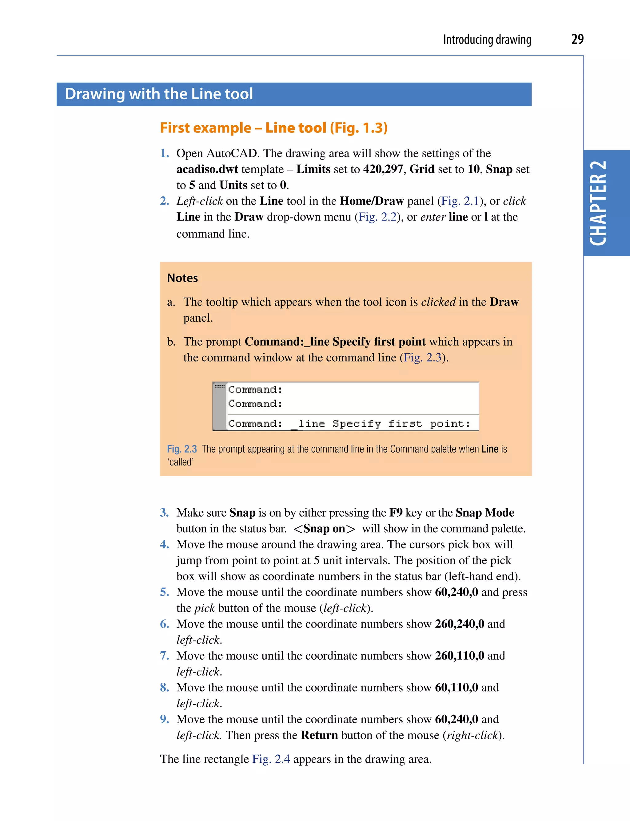
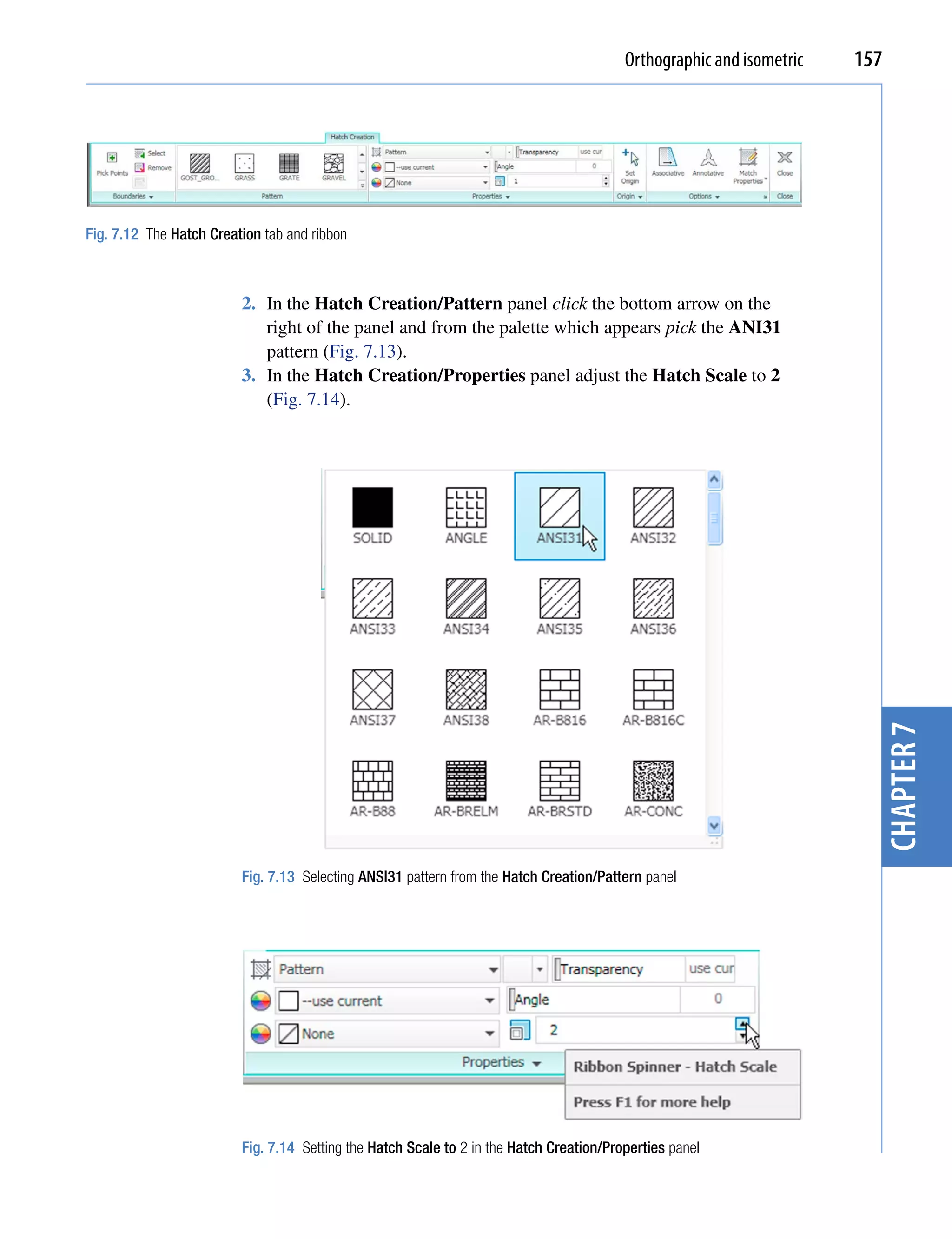
![30 Introduction to AutoCAD 2011
60,240,0 260,240,0
chapter 2
60,110,0 260,110,0
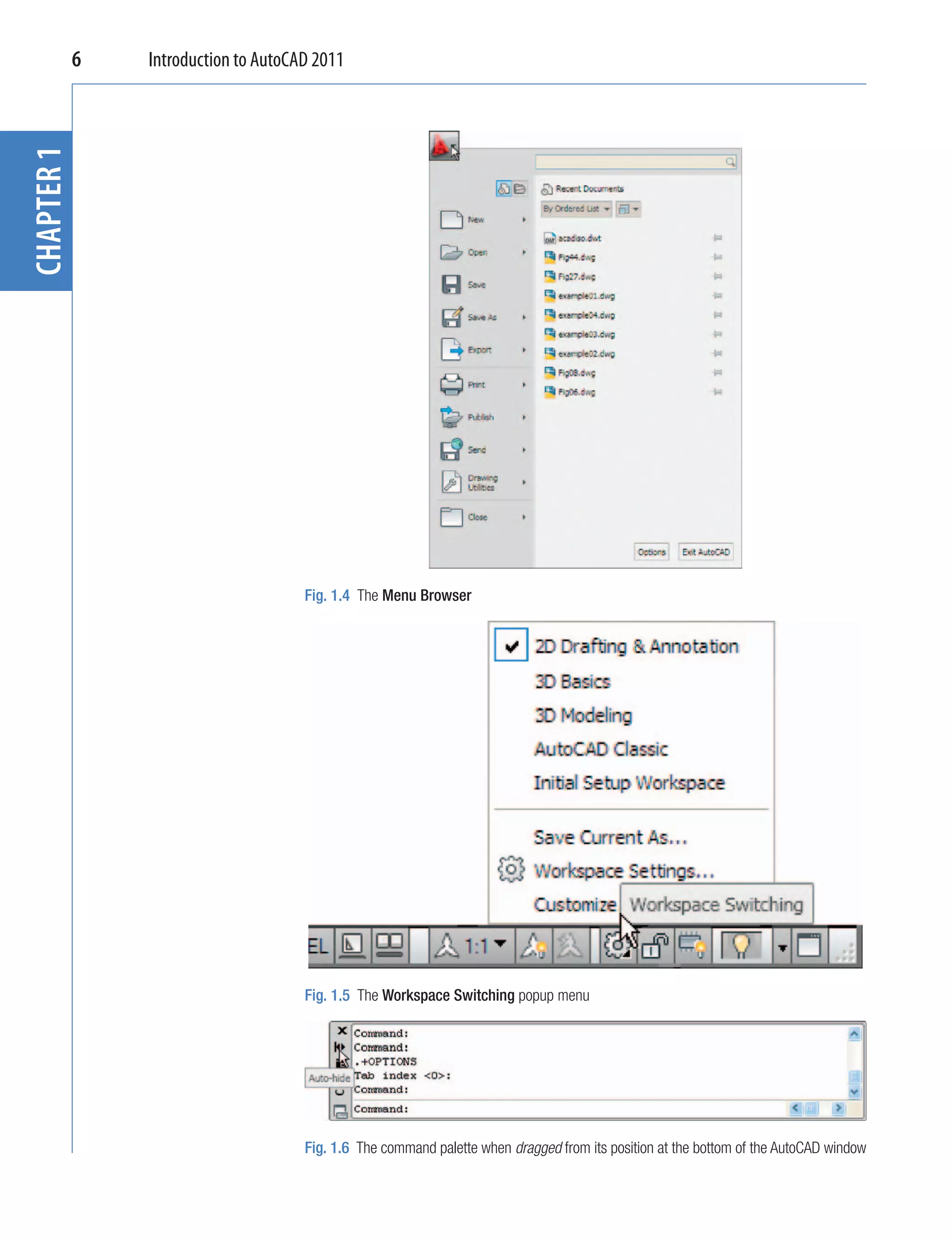
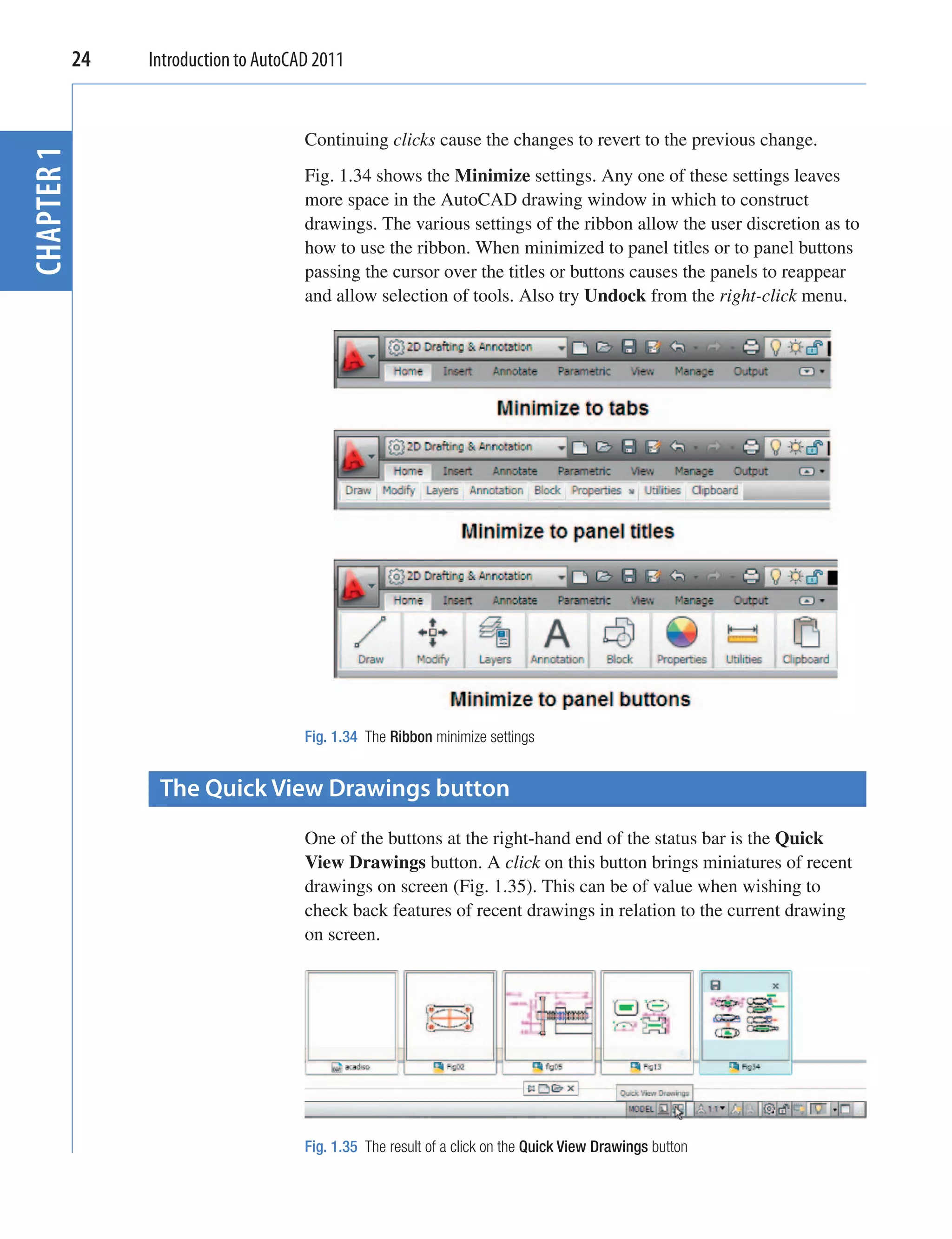
Fig. 2.4 First example – Line tool
Second example – Line tool (Fig. 2.6)
1. Clear the drawing from the screen with a click on the Close button of
the AutoCAD drawing area. Make sure it is not the AutoCAD 2011
window button.
2. The warning window Fig. 2.5 appears in the centre of the screen. Click
its No button.
Fig. 2.5 The AutoCAD warning window
3. Left-click New… button in the File drop-down menu and from the
Select template dialog which appears double-click on acadiso.dwt.
4. Left-click on the Line tool icon and enter figures as follows at each
prompt of the command line sequence:
Command:_line Specify first point: enter 80,235
right-click
Specify next point or [Undo]: enter 275,235
right-click
Specify next point or [Undo]: enter 295,210
right-click](https://image.slidesharecdn.com/introductiontoautocad2011-100614022653-phpapp02/75/Introduction-to-AutoCad-2011-29-2048.jpg)
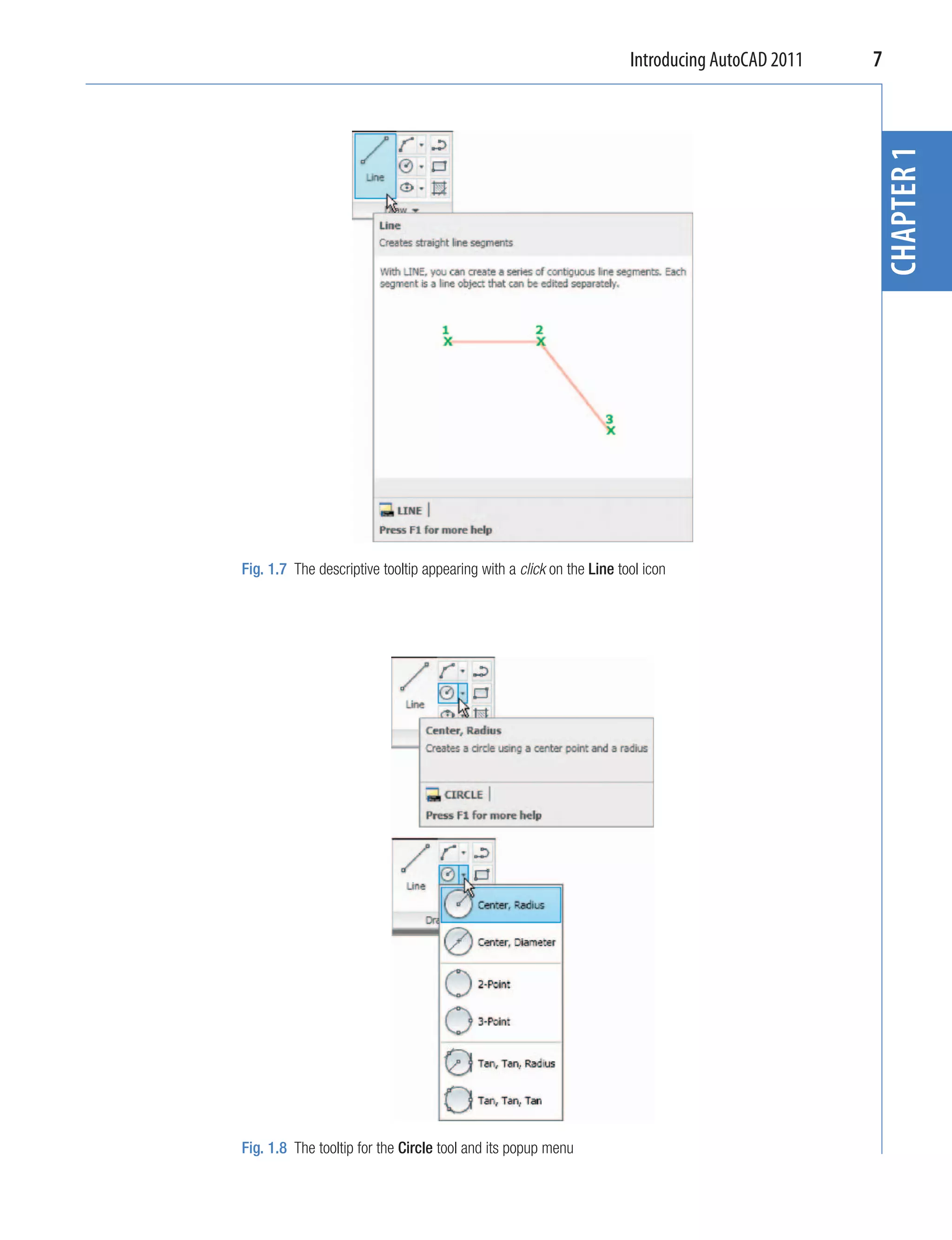
![Introducing drawing 31
Specify next point or [Close/Undo]: enter 295,100
right-click
Specify next point or [Close/Undo]: enter 230,100
right-click
Specify next point or [Close/Undo]: enter 230,70
chapter 2
right-click
Specify next point or [Close/Undo]: enter 120,70
right-click
Specify next point or [Close/Undo]: enter 120,100
right-click
Specify next point or [Close/Undo]: enter 55,100
right-click
Specify next point or [Close/Undo]: enter 55,210
right-click
Specify next point or [Close/Undo]: enter c
(Close) right-click
Command:
The result is as shown in Fig. 2.6.
80,235 275,235
55,210 295,210
120,100 230,100
55,100 295,100
120,70 230,70
Fig. 2.6 Second example – Line tool
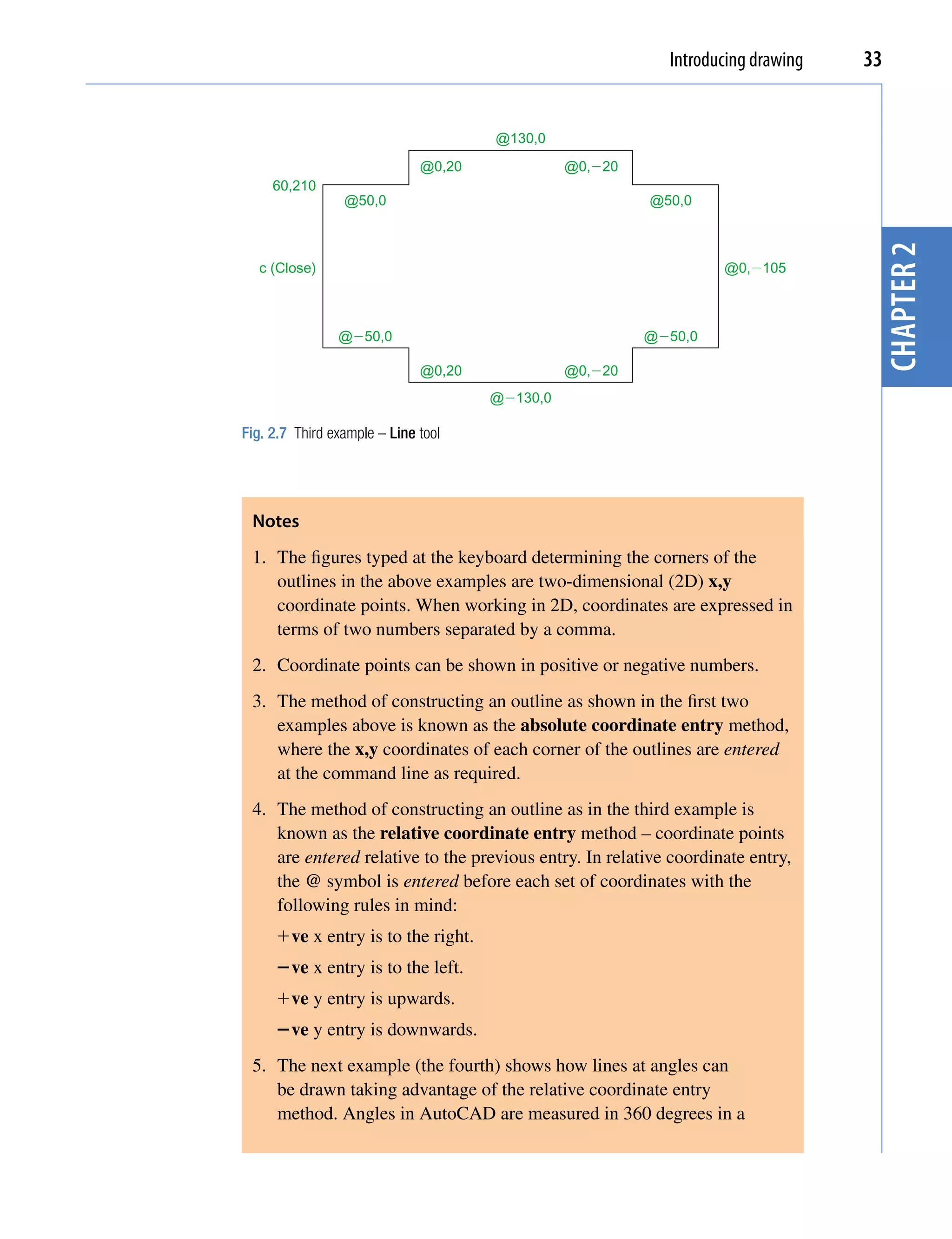
Third example – Line tool (Fig. 2.7)
1. Close the drawing and open a new acadiso.dwt window.
2. Left-click on the Line tool icon and enter figures as follows at each
prompt of the command line sequence:
Command:_line Specify first point: enter 60,210
right-click](https://image.slidesharecdn.com/introductiontoautocad2011-100614022653-phpapp02/75/Introduction-to-AutoCad-2011-30-2048.jpg)
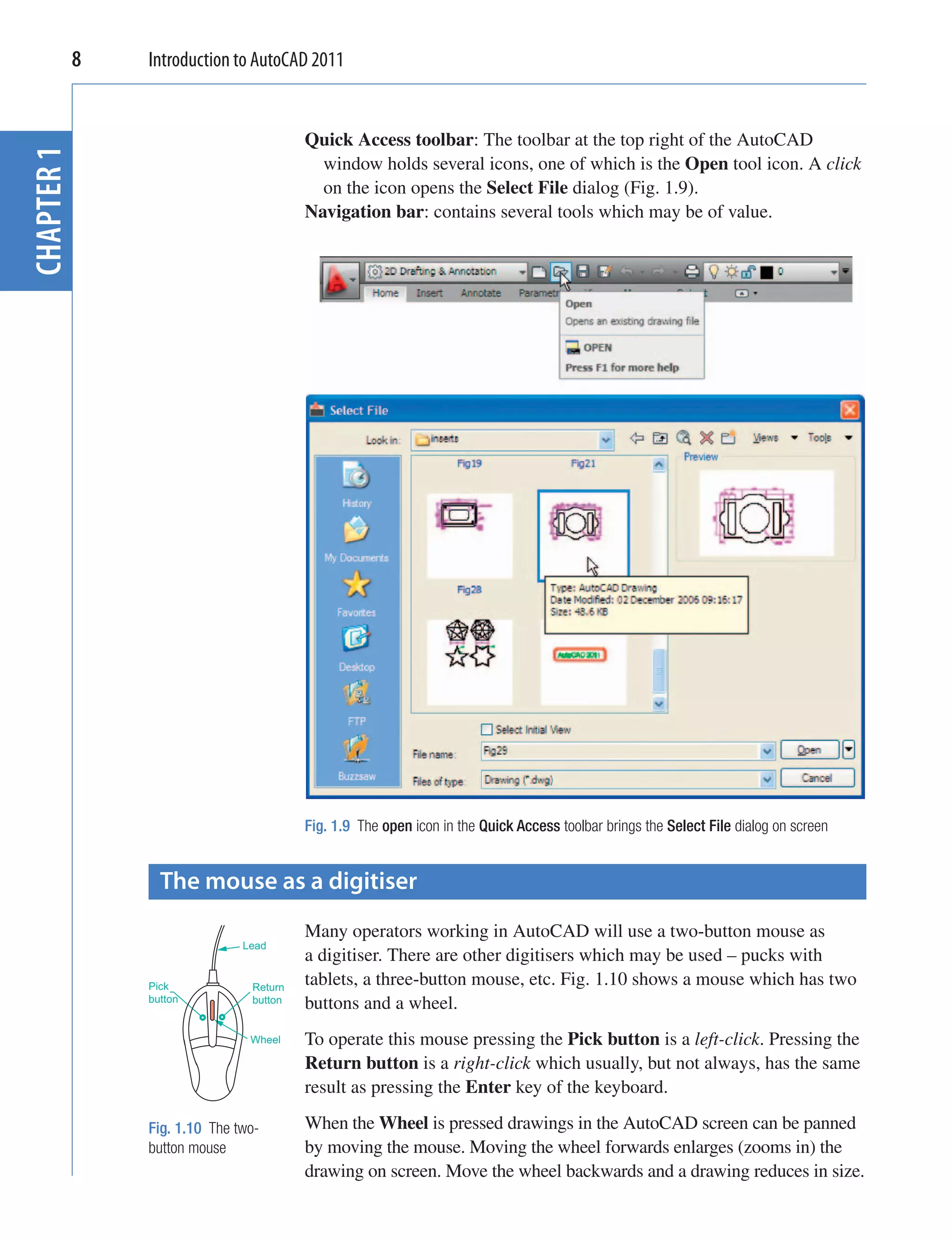
![32 Introduction to AutoCAD 2011
Specify next point or [Undo]: enter @50,0
right-click
Specify next point or [Undo]: enter @0,20
right-click
Specify next point or [Close/Undo]: enter @130,0
chapter 2
right-click
Specify next point or [Close/Undo]: enter @0,-20
right-click
Third example – Line tool (Fig. 2.7)
1. Close the drawing and open a new acadiso.dwt window.
2. Left-click on the Line tool icon and enter figures as follows at each
prompt of the command line sequence:
Command:_line Specify first point: enter 60,210
right-click
Specify next point or [Undo]: enter @50,0
right-click
Specify next point or [Undo]: enter @0,20
right-click
Specify next point or [Undo/Undo]: enter @130,0
right-click
Specify next point or [Undo/Undo]: enter @0,-20
right-click
Specify next point or [Undo/Undo]: enter @50,0
right-click
Specify next point or [Close/Undo]: enter @0,-105
right-click
Specify next point or [Close/Undo]: enter @-50,0
right-click
Specify next point or [Close/Undo]: enter @0,-20
right-click
Specify next point or [Close/Undo]: enter @-130,0
right-click
Specify next point or [Close/Undo]: enter @0,20
right-click
Specify next point or [Close/Undo]: enter @-50,0
right-click
Specify next point or [Close/Undo]: enter c
(Close) right-click
Command:
The result is as shown in Fig. 2.7.](https://image.slidesharecdn.com/introductiontoautocad2011-100614022653-phpapp02/75/Introduction-to-AutoCad-2011-31-2048.jpg)
![34 Introduction to AutoCAD 2011
counterclockwise (anticlockwise) direction (Fig. 2.8). The symbol
precedes the angle.
chapter 2
90�
135� 45�
180� 0�
225� 315�
270�
Fig. 2.8 The counterclockwise direction of measuring angles in AutoCAD
Fourth example – Line tool (Fig. 2.9)
1. Close the drawing and open a new acadiso.dwt window.
2. Left-click on the Line tool icon and enter figures as follows at each
prompt of the command line sequence:
Command:_line Specify first point: 70,230
Specify next point: @220,0
Specify next point: @0,-70
Specify next point or [Undo]: @115<225
Specify next point or [Undo]: @-60,0
Specify next point or [Close/Undo]: @115<135
Specify next point or [Close/Undo]: @0,70
Specify next point or [Close/Undo]: c (Close)
Command:
The result is as shown in Fig. 2.9.](https://image.slidesharecdn.com/introductiontoautocad2011-100614022653-phpapp02/75/Introduction-to-AutoCad-2011-33-2048.jpg)
![Introducing drawing 35
70,230 @220,0
c(Close)
@0,70 @0,�70
chapter 2
@
5
22
11
5�
5�
11
13
@
5
@�60,0
Fig. 2.9 Fourth example – Line tool
Fifth example – Line tool (Fig. 2.10)
Another method of constructing accurate drawings is by using a method
known as tracking. When Line is in use, as each Specify next point:
appears at the command line, a rubber-banded line appears from the last
point entered. Drag the rubber-band line in any direction and enter a
number at the keyboard, followed by a right-click. The line is drawn in the
dragged direction of a length in units equal to the entered number.
In this example because all lines are drawn in vertical or horizontal
directions, either press the F8 key or click the ORTHO button in the status
bar which will only allow drawing horizontally or vertically.
1. Close the drawing and open a new acadiso.dwt window.
2. Left-click on the Line tool icon and enter figures as follows at each
prompt of the command line sequence:
Command:_line Specify first point: enter 65,220
right-click
Specify next point: drag to right enter 240
right-click
Specify next point: drag down enter 145 right-click
Specify next point or [Undo]: drag left enter 65
right-click
Specify next point or [Undo]: drag upwards enter 25
right-click
Specify next point or [Close/Undo]: drag left
enter 120 right-click
Specify next point or [Close/Undo]: drag upwards
enter 25 right-click](https://image.slidesharecdn.com/introductiontoautocad2011-100614022653-phpapp02/75/Introduction-to-AutoCad-2011-34-2048.jpg)
![36 Introduction to AutoCAD 2011
Specify next point or [Close/Undo]: drag left
enter 55 right-click
Specify next point or [Close/Undo]: c (Close)
right-click
Command:
chapter 2
The result is as shown in Fig. 2.10.
240
65,220
c (Close)
145
55
25
120
25
65
Fig. 2.10 Fifth example – Line tool
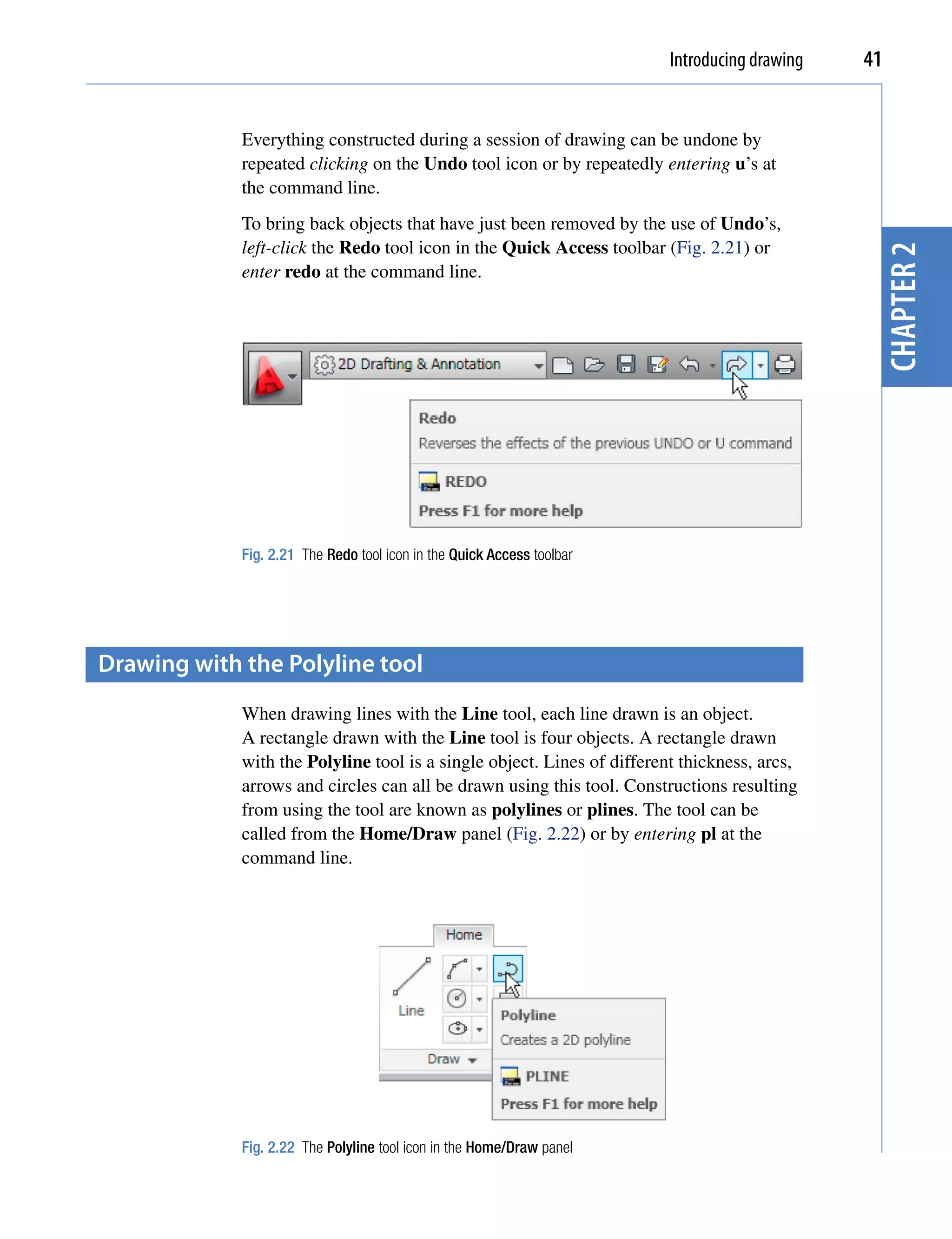
Drawing with the circle tool
First example – Circle tool (Fig. 2.13)
1. Close the drawing just completed and open the acadiso.dwt template.
2. Left-click on the Circle tool icon in the Home/Draw panel (Fig. 2.11).
Fig. 2.11 The Circle tool from the Home/Draw panel](https://image.slidesharecdn.com/introductiontoautocad2011-100614022653-phpapp02/75/Introduction-to-AutoCad-2011-35-2048.jpg)
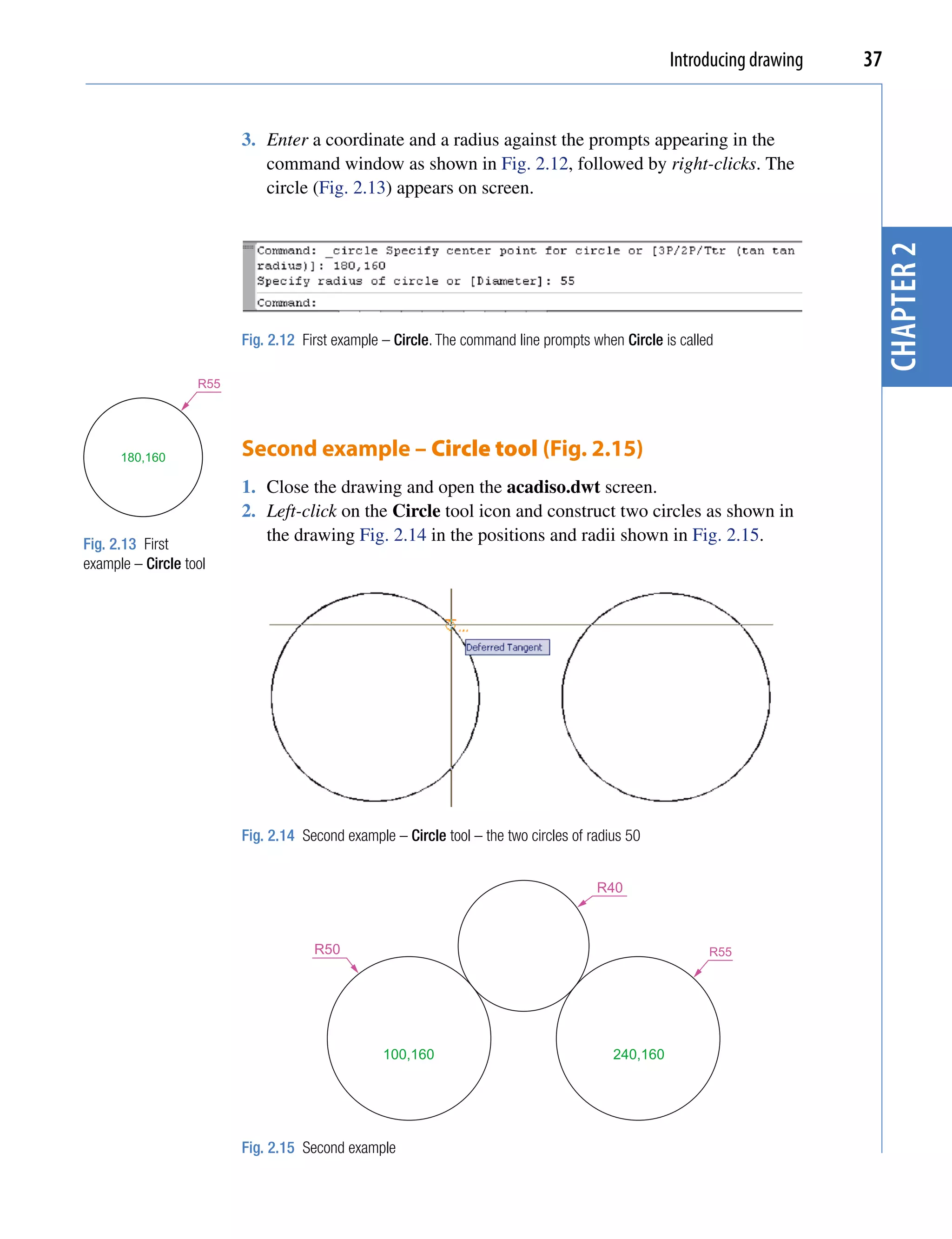
![38 Introduction to AutoCAD 2011
3. Click the Circle tool again and against the first prompt enter t (the
abbreviation for the prompt tan tan radius), followed by a right-click.
Command_circle Specify center point for circle or
[3P/2P/Ttr (tan tan radius]: enter t right-click
Specify point on object for first tangent of
chapter 2
circle: pick
Specify point on object for second tangent of
circle: pick
Specify radius of circle (50): enter 40 right-
click
Command:
The circle of radius 40 tangential to the two circles already drawn then
appears (Fig. 2.15).
Notes
1. When a point on either circle is picked a tip (Deferred Tangent)
appears. This tip will only appear when the Object Snap button is
set on with a click on its button in the status bar, or the F3 key of the
keyboard is pressed.
2. Circles can be drawn through 3 points or through 2 points entered at
the command line in response to prompts brought to the command line
by using 3P and 2P in answer to the circle command line prompts.
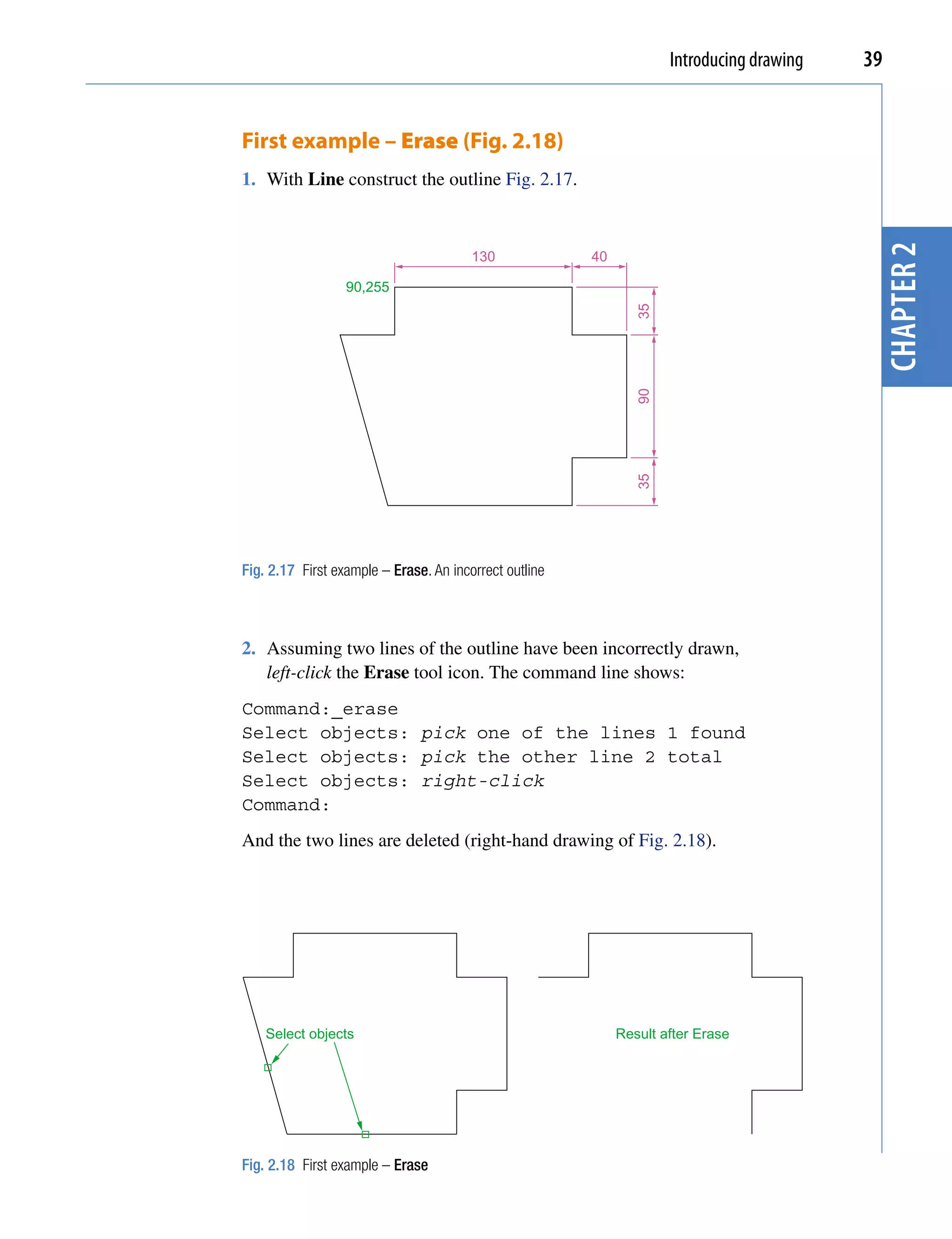
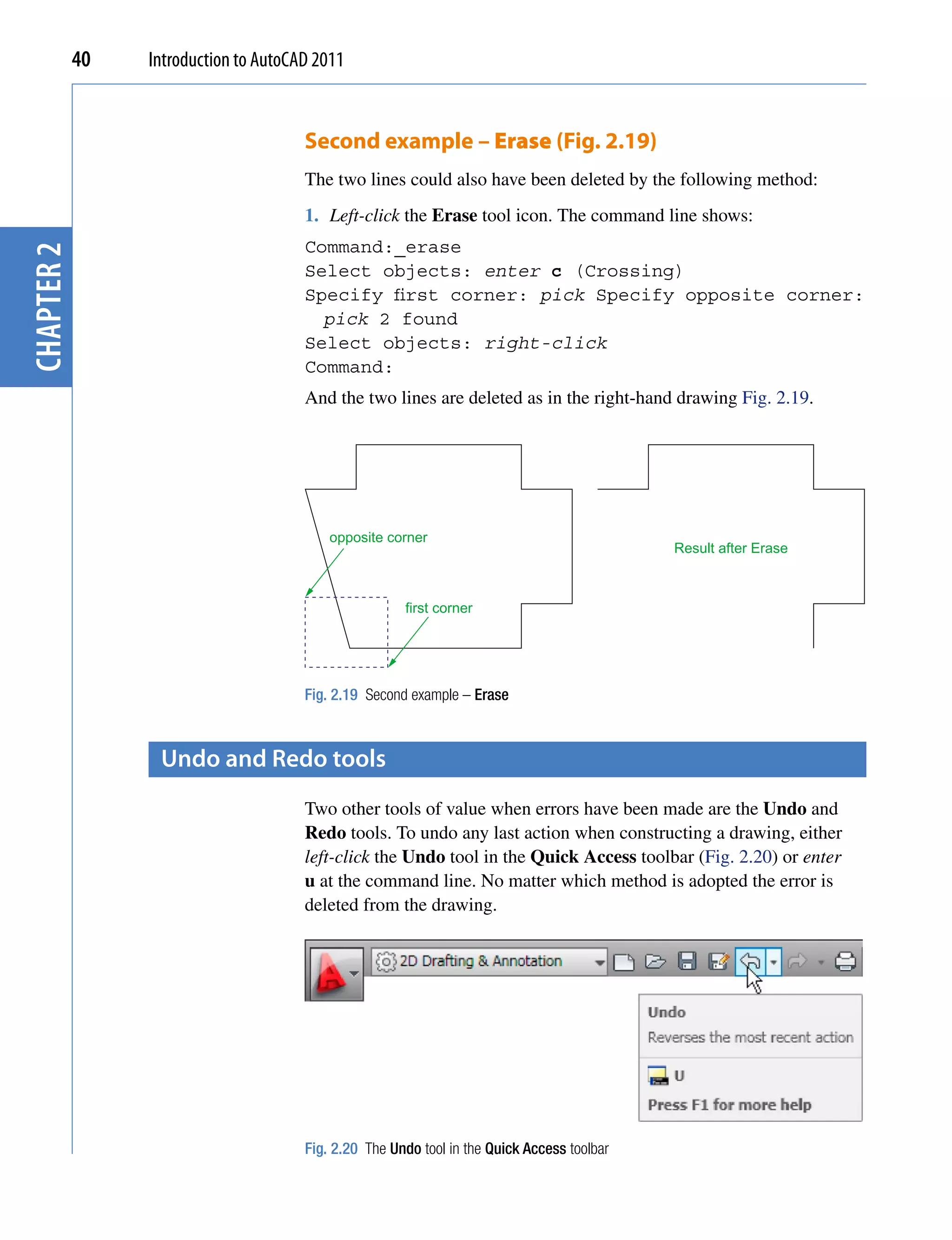
the erase tool
If an error has been made when using any of the AutoCAD 2011 tools,
the object or objects which have been incorrectly drawn can be deleted
with the Erase tool. The Erase tool icon can be selected from the Home/
Modify panel (Fig. 2.16) or by entering e at the command line.
Fig. 2.16 The Erase tool icon from the Home/Modify panel](https://image.slidesharecdn.com/introductiontoautocad2011-100614022653-phpapp02/75/Introduction-to-AutoCad-2011-37-2048.jpg)
![42 Introduction to AutoCAD 2011
First example – Polyline tool (Fig. 2.23)
In this example enter and right-click have not been included (Fig. 2.23).
Left-click the Polyline tool icon. The command line shows:
chapter 2
Command:_pline Specify start point: 30,250
Current line width is 0
Specify next point or [Arc/Halfwidth/Length/Undo/
Width]: 230,250
Specify next point or [Arc/Close/Halfwidth/Length/
Undo/Width]: 230,120
Specify next point or [Arc/Close/Halfwidth/Length/
Undo/Width]: 30,120
Specify next point or [Arc/Close/Halfwidth/Length/
Undo/Width]: c (Close)
Command:
30,250 230,250
30,120 230,120
Fig. 2.23 First example – Polyline tool
Notes
1. Note the prompts – Arc for constructing pline arcs, Close to close
an outline, Halfwidth to halve the width of a wide pline, Length
to enter the required length of a pline, Undo to undo the last pline
constructed Width to change the width of the pline.
2. Only the capital letter(s) of a prompt needs to be entered in upper or
lower case to make that prompt effective.
3. Other prompts will appear when the Polyline tool is in use as will be
shown in later examples.](https://image.slidesharecdn.com/introductiontoautocad2011-100614022653-phpapp02/75/Introduction-to-AutoCad-2011-41-2048.jpg)
![Introducing drawing 43
Second example – Polyline tool (Fig. 2.24)
This will be a long sequence, but it is typical of a reasonably complex
drawing using the Polyline tool. In the following sequences, when a
prompt line is to be repeated, the prompts in square brackets ([]) will be
replaced by [prompts] (Fig. 2.24).
chapter 2
40,250 160,250 260,250
260,180
260,120
40,120 160,120
Fig. 2.24 Second example – Polyline tool
Left-click the Polyline tool icon. The command line shows:
Command:_pline Specify start point: 40,250
Current line width is 0
Specify next point or [Arc/Halfwidth/Length/Undo/
Width]: w (Width)
Specify starting width <0>: 5
Specify ending width <5>: right-click
Specify next point or [Arc/Close/Halfwidth/Length/
Undo/Width]: 160,250
Specify next point or [prompts]: h (Halfwidth)
Specify starting half-width <2.5>: 1
Specify ending half-width <1>: right-click
Specify next point or [prompts]: 260,250
Specify next point or [prompts]: 260,180
Specify next point or [prompts]: w (Width)
Specify starting width <1>: 10
Specify ending width <10>: right-click
Specify next point or [prompts]: 260,120
Specify next point or [prompts]: h (Halfwidth)
Specify starting half-width <5>: 2
Specify ending half-width <2>: right-click
Specify next point or [prompts]: 160,120
Specify next point or [prompts]: w (Width)](https://image.slidesharecdn.com/introductiontoautocad2011-100614022653-phpapp02/75/Introduction-to-AutoCad-2011-42-2048.jpg)
![44 Introduction to AutoCAD 2011
Specify starting width <4>: 20
Specify ending width <20>: right-click
Specify next point or [prompts]: 40,120
Specify starting width <20>: 5
Specify ending width <5>: right-click
chapter 2
Specify next point or [prompts]: c (Close)
Command:
Third example – Polyline tool (Fig. 2.25)
Left-click the Polyline tool icon. The command line shows:
Command:_pline Specify start point: 50,220
Current line width is 0
[prompts]: w (Width)
Specify starting width <0>: 0.5
Specify ending width <0.5>: right-click
Specify next point or [prompts]: 120,220
Specify next point or [prompts]: a (Arc)
Specify endpoint of arc or [prompts]: s (second pt)
Specify second point on arc: 150,200
Specify end point of arc: 180,220
Specify end point of arc or [prompts]: l (Line)
Specify next point or [prompts]: 250,220
Specify next point or [prompts]: 260,190
Specify next point or [prompts]: a (Arc)
Specify endpoint of arc or [prompts]: s (second pt)
Specify second point on arc: 240,170
Specify end point of arc: 250,160
Specify end point of arc or [prompts]: l (Line)
Specify next point or [prompts]: 250,150
Specify next point or [prompts]: 250,120
And so on until the outline Fig. 2.25 is completed.
50,220 120,220 180,220 250,220
50,190 150,200 250,190
60,170 240,170
50,150 150,140 250,150
50,120 120,120 180,120 250,120
Fig. 2.25 Third example – Polyline tool](https://image.slidesharecdn.com/introductiontoautocad2011-100614022653-phpapp02/75/Introduction-to-AutoCad-2011-43-2048.jpg)
![Introducing drawing 45
Fourth example – Polyline tool (Fig. 2.26)
Left-click the Polyline tool icon. The command line shows:
Command:_pline Specify start point: 80,170
Current line width is 0
chapter 2
Specify next point or [prompts]: w (Width)
Specify starting width <0>: 1
Specify ending width <1>: right-click
Specify next point or [prompts]: a (Arc)
Specify endpoint of arc or [prompts]: s (second pt)
Specify second point on arc: 160,250
Specify end point of arc: 240,170
Specify end point of arc or [prompts]: cl (CLose)
Command:
And the circle Fig. 2.26 is formed.
160,250
80,170 240,170
Fig. 2.26 Fourth example – Polyline tool
Fifth example – Polyline tool (Fig. 2.27)
Left-click the Polyline tool icon. The command line shows:
Command:_pline Specify start point: 60,180
Current line width is 0
Specify next point or [prompts]: w (Width)
Specify starting width <0>: 1
Specify ending width <1>: right-click
Specify next point or [prompts]: 190,180
Specify next point or [prompts]: w (Width)
Specify starting width <1>: 20
Specify ending width <20>: 0
Specify next point or [prompts]: 265,180
Specify next point or [prompts]: right-click
Command:](https://image.slidesharecdn.com/introductiontoautocad2011-100614022653-phpapp02/75/Introduction-to-AutoCad-2011-44-2048.jpg)

![52 Introduction to AutoCAD 2011
55,250
10,220 100,220 140,215 260,215
First example 320,210 420,210
Center is 200,190 Radius�75
Second example Third example
Fig. 3.5 Examples – Arc tool
chapter 3
First example – Arc tool (Fig. 3.5)
Left-click the Arc tool icon. The command line shows:
Command:_arc Specify start point of arc or
[Center]: 100,220
Specify second point of arc or [Center/End]:
Fig. 3.4 The Arc tool 55,250
flyout in the Home/ Specify end point of arc: 10,220
Draw panel
Command:
Second example – Arc tool (Fig. 3.5)
Command:right-click brings back the Arc sequence
ARC Specify start point of arc or [Center]: c
(Center)
Specify center point of arc: 200,190
Specify start point of arc: 260,215
Specify end point of arc or [Angle/chord Length]:
140,215
Command:
Third example – Arc tool (Fig. 3.5)
Command:right-click brings back the Arc sequence
ARC Specify start point of arc or [Center]:
420,210
Specify second point of arc or [Center/End]:
e (End)
Specify end point of arc: 320,210
Specify center point of arc or [Angle/Direction/
Radius]: r (Radius)
Specify radius of arc: 75
Command:](https://image.slidesharecdn.com/introductiontoautocad2011-100614022653-phpapp02/75/Introduction-to-AutoCad-2011-51-2048.jpg)
![Draw tools, Object Snap and Dynamic Input 53
the ellipse tool
Ellipses can be regarded as what is seen when a circle is viewed from
directly in front of the circle and the circle rotated through an angle about
its horizontal diameter. Ellipses are measured in terms of two axes – a
major axis and a minor axis, the major axis being the diameter of the
circle and the minor axis being the height of the ellipse after the circle has
been rotated through an angle (Fig. 3.6).
chapter 3
major axis minor axis
Diameter
Circle rotated
through 60� Ellipse as
seen from
Circle as Circle as seen direction of arrow
seen from from direction
a side of arrow
Fig. 3.6 An ellipse can be regarded as viewing a rotated circle
To call the Ellipse tool, click on its tool icon in the Home/Draw panel
(Fig. 3.7), click its name in the Draw drop-down menu or enter a or arc at
the command line.
First example – Ellipse (Fig. 3.8)
Left-click the Ellipse tool icon. The command line shows:
Command:_ellipse
Fig. 3.7 The Ellipse Specify axis endpoint of elliptical arc or
tool icon flyout in the [Center]: 30,190
Home/Draw panel Specify other endpoint of axis: 150,190
Specify distance to other axis or [Rotation] 25
Command:
Second example – Ellipse (Fig. 3.8)
In this second example, the coordinates of the centre of the ellipse (the
point where the two axes intersect) are entered, followed by entering
coordinates for the end of the major axis, followed by entering the units
for the end of the minor axis.
Command:right-click
ELLIPSE](https://image.slidesharecdn.com/introductiontoautocad2011-100614022653-phpapp02/75/Introduction-to-AutoCad-2011-52-2048.jpg)
![54 Introduction to AutoCAD 2011
Specify axis endpoint of elliptical arc or
[Center]: c
Specify center of ellipse: 260,190
Specify endpoint of axis: 205,190
Specify distance to other axis or
[Rotation]: 30
Command:
Third example – Ellipse (Fig. 3.8)
chapter 3
In this third example, after setting the positions of the ends of the major
axis, the angle of rotation of the circle from which an ellipse can be
obtained is entered (Fig. 3.8).
30
25
30,190 150,190 205,190
260,190
First example
Second example
30,100 Rotation�45� 120,100
Third example
Fig. 3.8 Examples – Ellipse
Command: right-click
ELLIPSE
Specify axis endpoint of elliptical arc or
[Center]: 30,100
Specify other endpoint of axis: 120,100
Specify distance to other axis or [Rotation]:
r (Rotation)
Specify rotation around major axis: 45
Command:
saving drawings
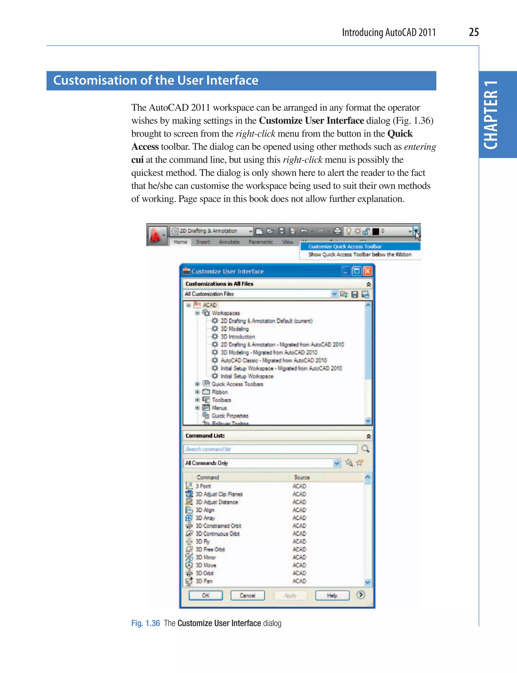
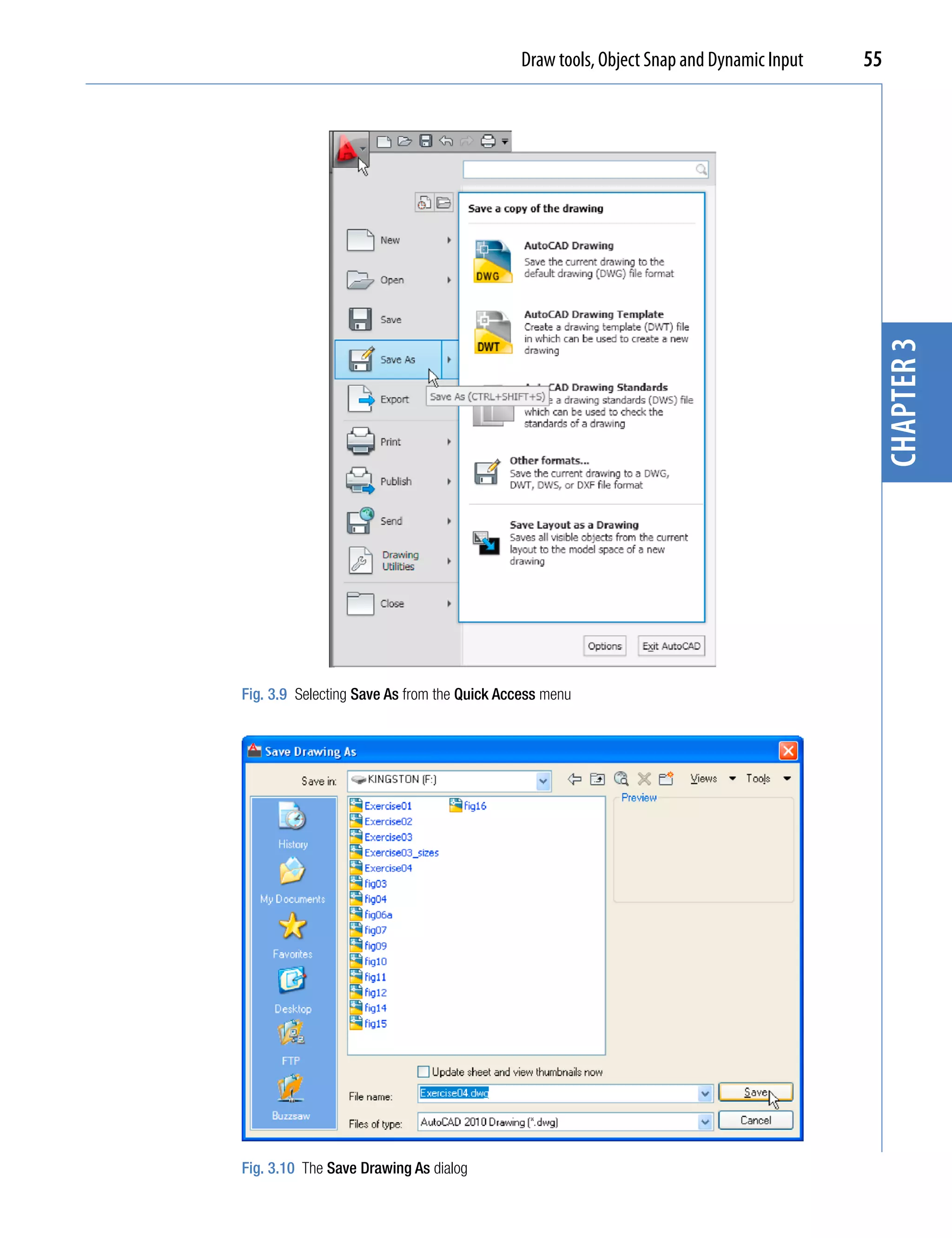
Before going further it is as well to know how to save the drawings
constructed when answering examples and exercises in this book. When a
drawing has been constructed, left-click on Save As in the menu appearing
with a left-click on the AutoCAD icon at the top left-hand corner of the
window (Fig. 3.9). The Save Drawing As dialog appears (Fig. 3.10).](https://image.slidesharecdn.com/introductiontoautocad2011-100614022653-phpapp02/75/Introduction-to-AutoCad-2011-53-2048.jpg)
![56 Introduction to AutoCAD 2011
Unless you are the only person using the computer on which the drawing
has been constructed, it is best to save work to a USB memory stick or other
form of temporary saving device. To save a drawing to a USB memory stick:
1. Place a memory stick in a USB drive.
2. In the Save in: field of the dialog, click the arrow to the right of the
field and from the popup list select KINGSTON [F:] (the name of my
USB drive and stick).
3. In the File name: field type a name. The file name extension .dwg does
not need to be typed – it will be added to the file name.
chapter 3
4. Left-click the Save button of the dialog. The drawing will be saved with the
file name extension .dwg – the AutoCAD file name extension (Fig. 3.10).
snap
In previous chapters, several methods of constructing accurate drawings
have been described – using Snap, absolute coordinate entry, relative
coordinate entry and tracking. Other methods of ensuring accuracy
between parts of constructions are by making use of Object Snaps
(Osnaps).
Snap Mode, Grid Display and Object Snaps can be toggled on/off from
the buttons in the status bar or by pressing the keys, F9 (Snap Mode),
F7 (Grid Display) and F3 (Object Snap).
object snaps (osnaps)
Object Snaps allow objects to be added to a drawing at precise positions in
relation to other objects already on screen. With Object Snaps, objects can
be added to the end points, midpoints, to intersections of objects, to centres
and/or quadrants of circles and so on. Object Snaps also override snap
points even when snap is set on.
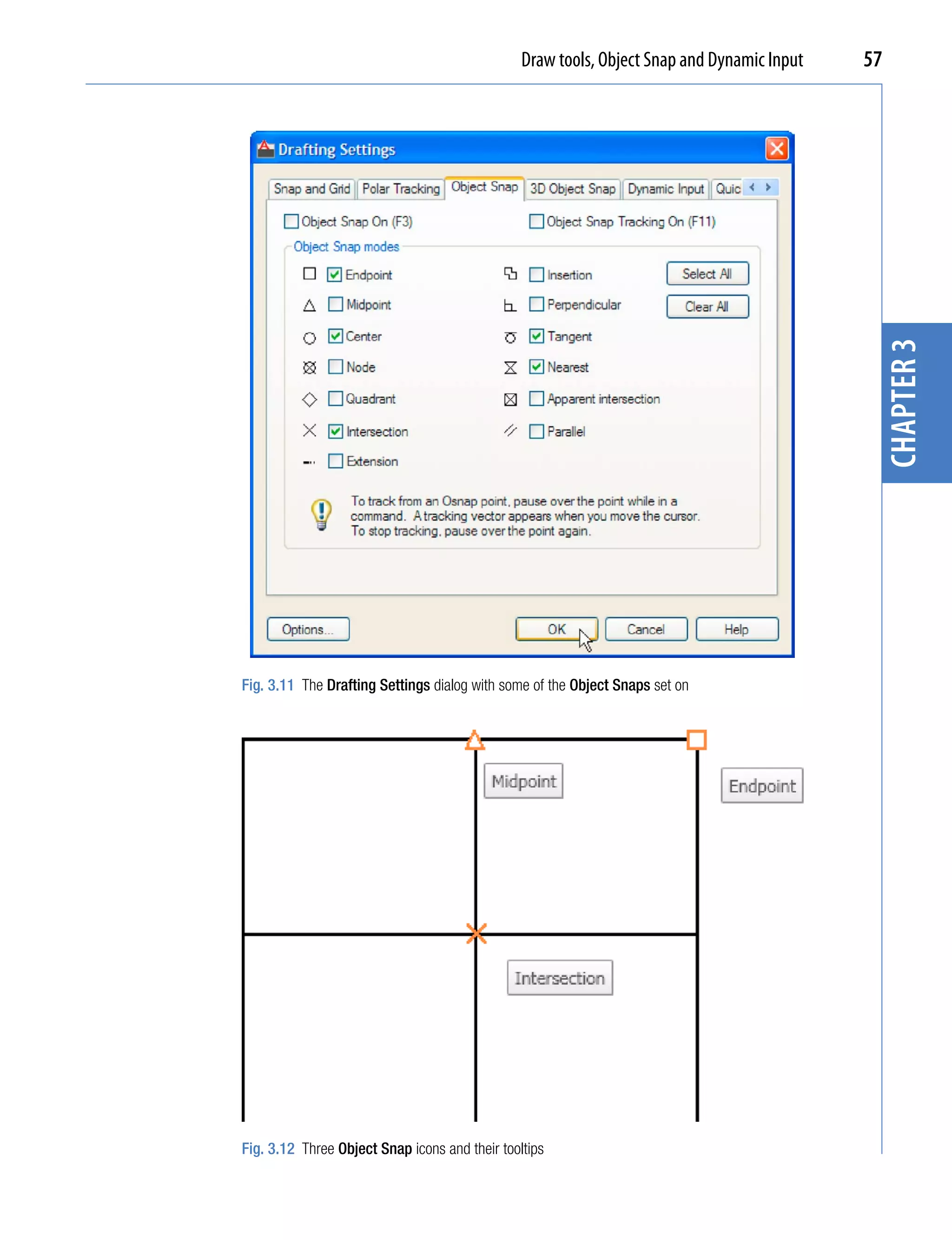
To set Object Snaps – at the command line:
Command: enter os
And the Drafting Settings dialog appears (Fig. 3.11). Click the Object
Snap tab in the upper part of the dialog and click the check boxes to the
right of the Object Snap names to set them on (or off in on).
When Object Snaps are set ON, as outlines are constructed using Object
Snap icons and their tooltips appear as indicated in Fig. 3.12.](https://image.slidesharecdn.com/introductiontoautocad2011-100614022653-phpapp02/75/Introduction-to-AutoCad-2011-55-2048.jpg)
![58 Introduction to AutoCAD 2011
It is sometimes advisable not to have Object Snaps set on in the
Drafting Settings dialog, but to set Object Snap off and use Object
Snap abbreviations at the command line when using tools. The following
examples show the use of some of these abbreviations. Object Snaps can
be toggled on/off by pressing the F3 key of the keyboard.
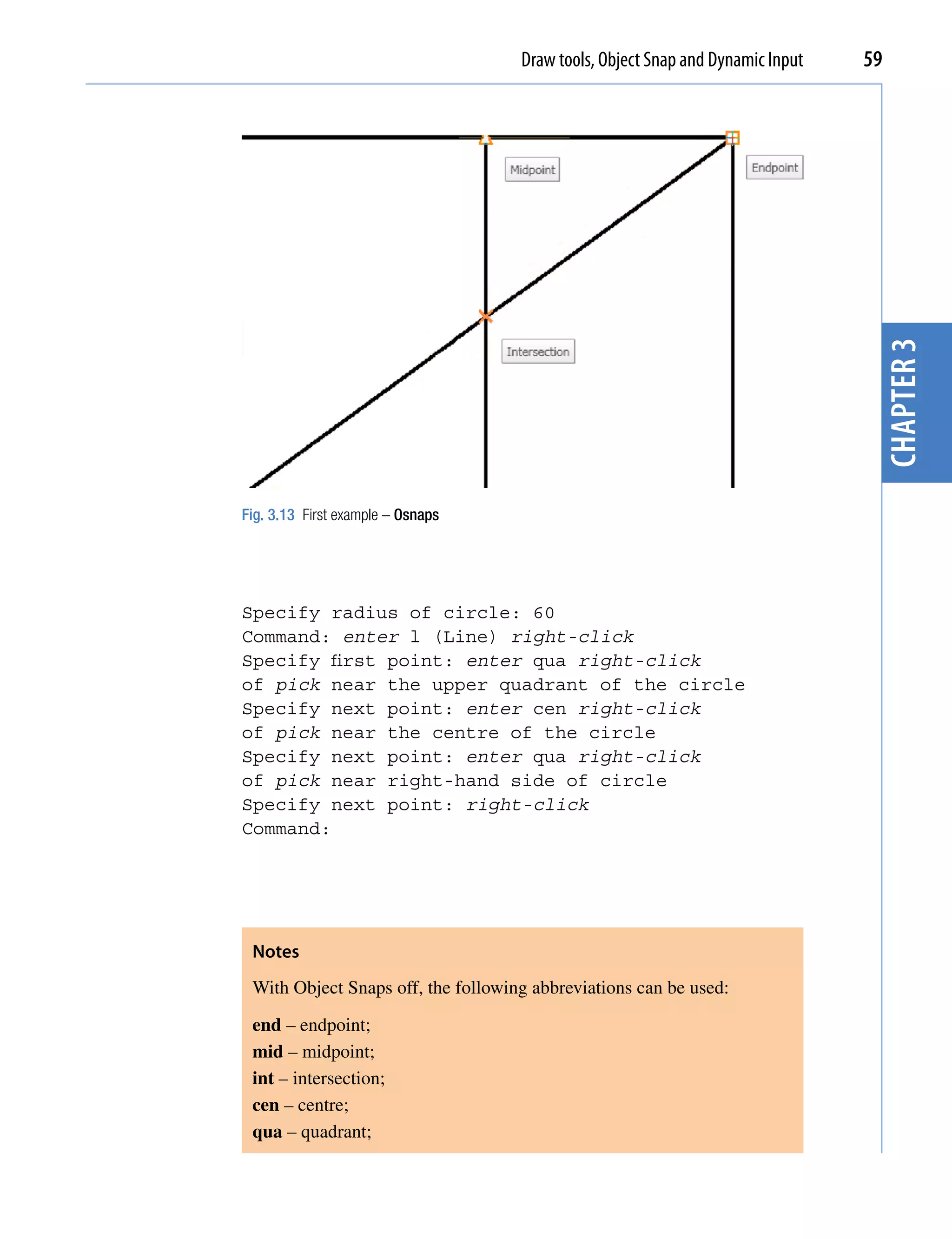
First example – Object Snap (Fig. 3.13)
Call the Polyline tool:
chapter 3
Command:_pline
Specify start point: 50,230
[prompts]: w (Width)
Specify starting width: 1
Specify ending width <1>: right-click
Specify next point: 260,230
Specify next point: right-click
Command: right-click
PLINE
Specify start point: pick the right-hand end of
the pline
Specify next point: 50,120
Specify next point: right-click
Command: right-click
PLINE
Specify start point: pick near the middle of first
pline
Specify next point: 155,120
Specify next point: right-click
Command: right-click
PLINE
Specify start point: pick the plines at their
intersection
Specify start point: right-click
Command:
The result is shown in Fig. 3.13. In this illustration the Object Snap
tooltips are shown as they appear when each object is added to the outline.
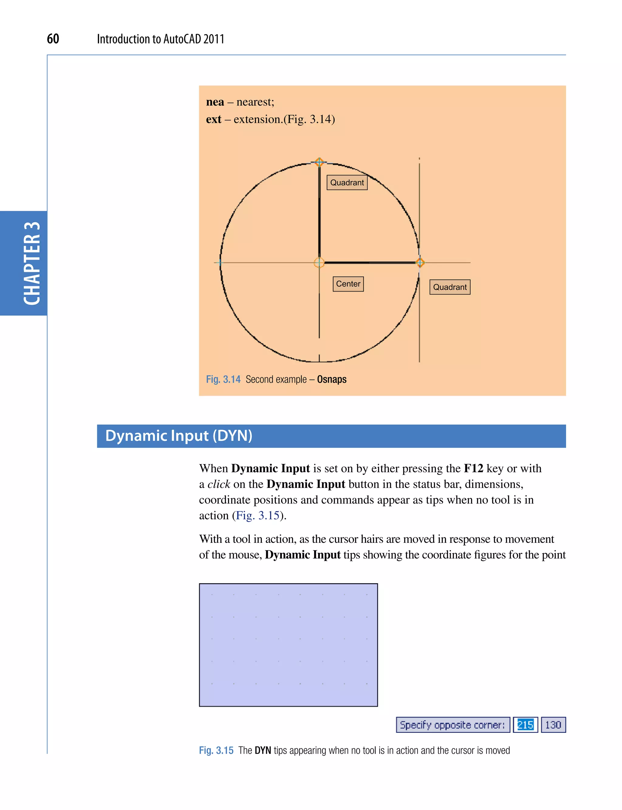
Second example – Object Snap abbreviations
(Fig. 3.14)
Call the Circle tool:
Command:_circle
Specify center point for circle: 180,170](https://image.slidesharecdn.com/introductiontoautocad2011-100614022653-phpapp02/75/Introduction-to-AutoCad-2011-57-2048.jpg)
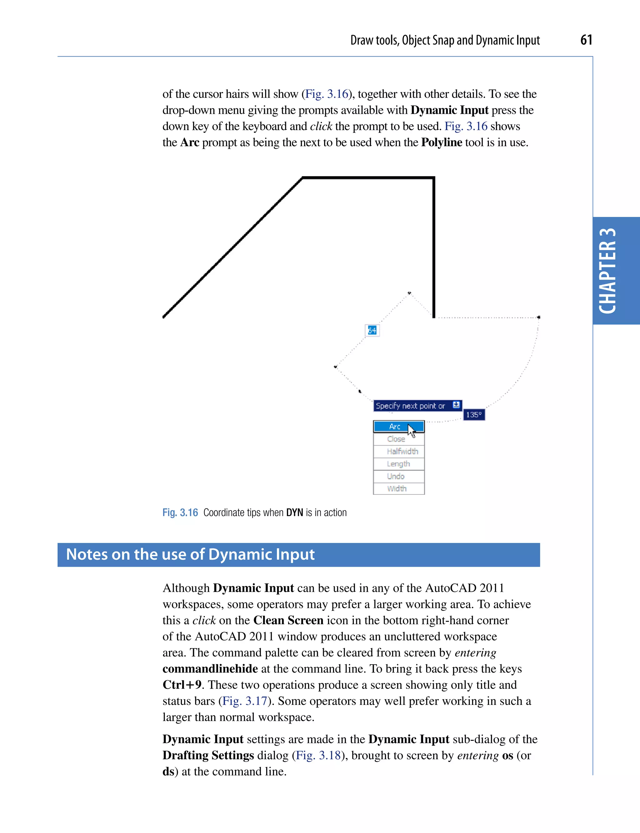
![Draw tools, Object Snap and Dynamic Input 69
examples of using other Draw tools
Polygon tool (Fig. 3.37)
Call the Polygon tool – either with a click on its tool icon in the Home/
Draw panel (Fig. 3.1, page 69), from the Draw drop-down menu, or by
entering pol or polygon at the command line. No matter how the tool is
called, the command line shows:
Command:_polygon Enter number of sides <4>: 6
chapter 3
Specify center of polygon or [Edge]: 60,210
Enter an option [Inscribed in circle/Circumscribed
about circle] <I>: right-click (accept Inscribed)
Specify radius of circle: 60
Command:
1. In the same manner construct a 5-sided polygon of centre 200,210 and
of radius 60.
2. Then, construct an 8-sided polygon of centre 330,210 and radius 60.
3. Repeat to construct a 9-sided polygon circumscribed about a circle of
radius 60 and centre 60,80.
4. Construct yet another polygon with 10 sides of radius 60 and of centre
200,80.
5. Finally another polygon circumscribing a circle of radius 60, of centre
330,80 and sides 12.
The result is shown in Fig. 3.37.
Inscribing
circle
5-sided 8-sided
6-sided octagon
pentagon
hexagon
Circumscribing
circle
9-sided
nonagon 10-sided 12-sided
decagon duodecagon
Fig. 3.37 First example – Polygon tool](https://image.slidesharecdn.com/introductiontoautocad2011-100614022653-phpapp02/75/Introduction-to-AutoCad-2011-68-2048.jpg)
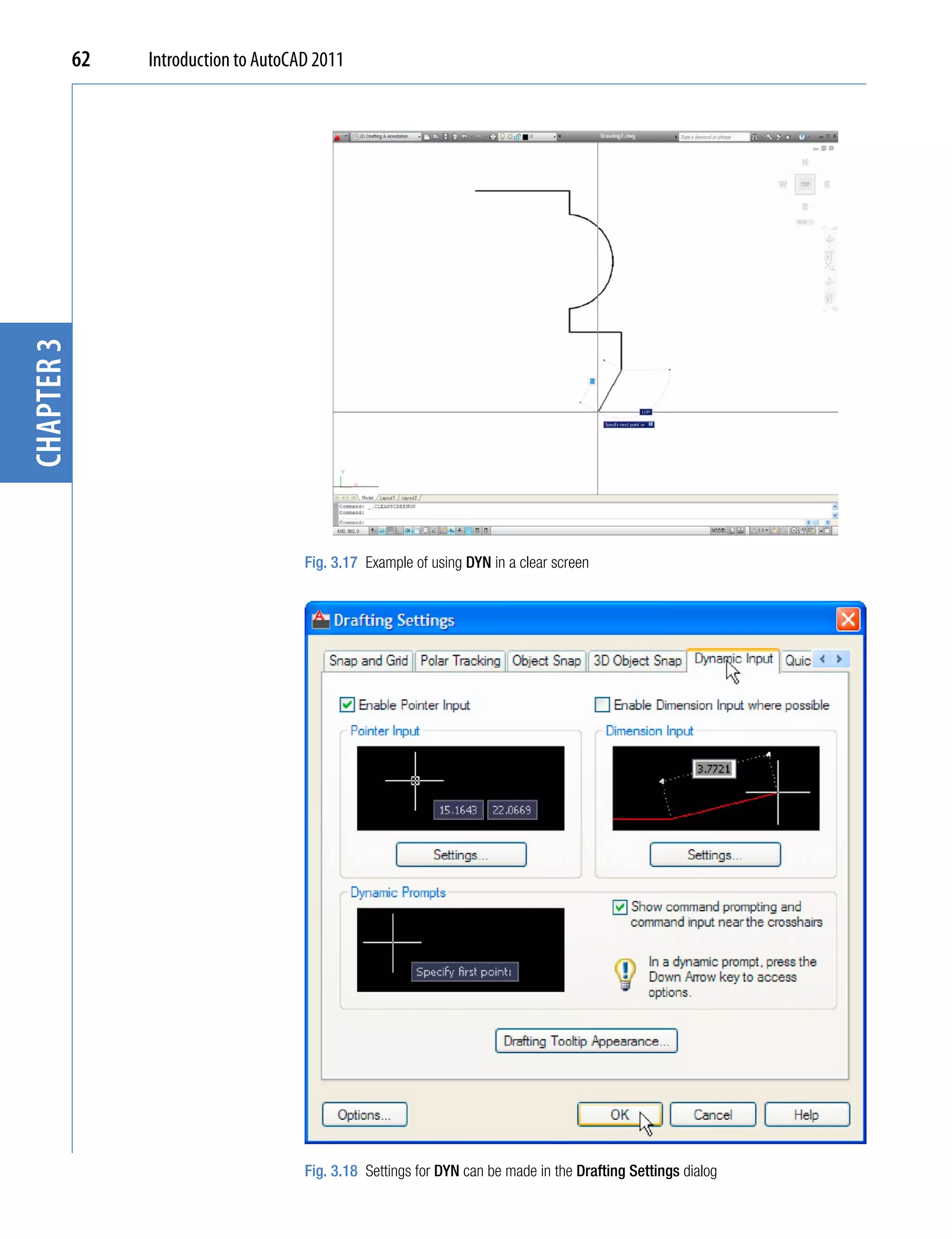
![70 Introduction to AutoCAD 2011
Rectangle tool – first example (Fig. 3.39)
Call the Rectangle tool – either with a click on its tool icon in the Home/
Draw panel (Fig. 3.38) by entering rec or rectangle at the command
line. The tool can be also called from the Draw drop-down menu. The
command line shows (Fig. 3.39):
Fig. 3.38 The
Rectangle tool from 25,240 200,240
chapter 3
the Home/Draw panel
Chamfers
15 and 15
160,160 300,160
20,120 200,120
Width�4
Width�2 Chamfers
Fileets�R15 10 and 15
160,30 315,25
Fig. 3.39 Examples – Rectangle tool
Command:_rectang
Specify first corner point or [Chamfer/
Elevation/Fillet/Thickness/Width]: 25,240
Specify other corner point or [Area/Dimensions/
Rotation]: 160,160
Command:
Rectangle tool – second example (Fig. 3.39)
Command:_rectang
[prompts]: c (Chamfer)
Specify first chamfer distance for rectangles
<0>: 15
Specify first chamfer distance for rectangles <15>:
right-click
Specify first corner point: 200,240
Specify other corner point: 300,160
Command:](https://image.slidesharecdn.com/introductiontoautocad2011-100614022653-phpapp02/75/Introduction-to-AutoCad-2011-69-2048.jpg)
![Draw tools, Object Snap and Dynamic Input 71
Rectangle tool – third example (Fig. 3.39)
Command: _rectang
Specify first corner point or [Chamfer/Elevation/
Fillet/Thickness/Width]: f (Fillet)
Specify fillet radius for rectangles <0>: 15
Specify first corner point or [Chamfer/Elevation/
Fillet/Thickness/Width]: w (Width)
Specify line width for rectangles <0>: 1
chapter 3
Specify first corner point or [Chamfer/Elevation/
Fillet/Thickness/Width]: 20,120
Specify other corner point or [Area/Dimensions/
Rotation]: 160,30
Command:
Rectangle – fourth example (Fig. 3.39)
Command:_rectang
Specify first corner point or [Chamfer/Elevation/
Fillet/Thickness/Width]: w (Width)
Specify line width for rectangles <0>: 4
Specify first corner point or [Chamfer/Elevation/
Fillet/Thickness/Width]: c (Chamfer)
Specify first chamfer distance for rectangles <0>: 15
Specify second chamfer distance for rectangles
<15>: right-click
Specify first corner point: 200,120
Specify other corner point: 315,25
Command:
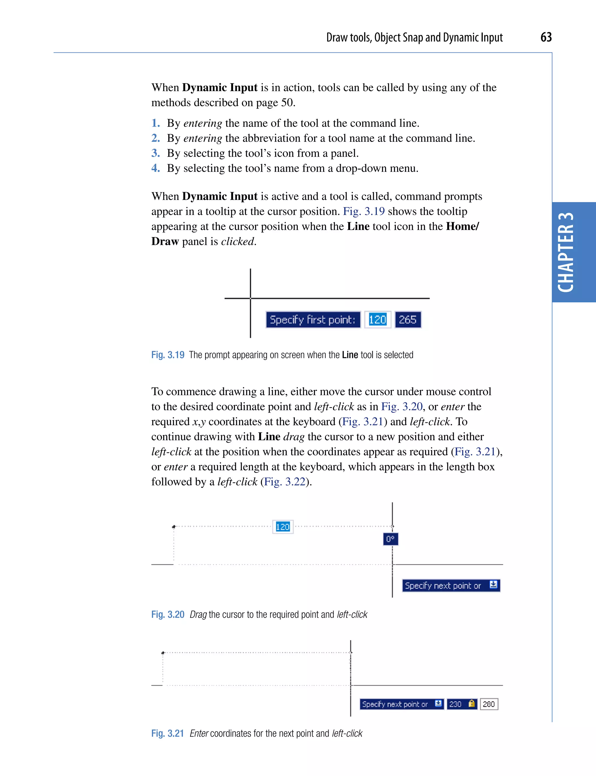
the polyline edit tool
The Polyline Edit tool is a valuable tool for the editing of polylines.
First example – Polyline Edit (Fig. 3.42)
1. With the Polyline tool construct the outlines 1 to 6 of Fig. 3.40.
2. Call the Edit Polyline tool either from the Home/Modify panel
(Fig. 3.41) or from the Modify drop-down menu, or by entering pe or
pedit at the command line, which then shows:
Command: enter pe
PEDIT Select polyline or [Multiple]: pick pline 2](https://image.slidesharecdn.com/introductiontoautocad2011-100614022653-phpapp02/75/Introduction-to-AutoCad-2011-70-2048.jpg)
![72 Introduction to AutoCAD 2011
1 2 3
Pline rectangel
120�80
4 5 6
chapter 3
Fig. 3.40 Examples – Edit Polyline – the plines to be edited
Fig. 3.41 Calling Edit Polyline from the Home/Modify panel
Enter an option [Open/Join/Width/Edit vertex/Fit/
Spline/Decurve/Ltype gen/Reverse/Undo]:
w (Width)
Specify new width for all segments: 2
Enter an option [Open/Join/Width/Edit vertex/Fit/
Spline/Decurve/Ltype gen/Reverse/Undo]: right-
click
Command:
3. Repeat with pline 3 and pedit to Width 10.
4. Repeat with line 4 and enter s (Spline) in response to the prompt line:
Enter an option [Open/Join/Width/Edit vertex/Fit/
Spline/Decurve/Ltype gen/Reverse/Undo]: enter s
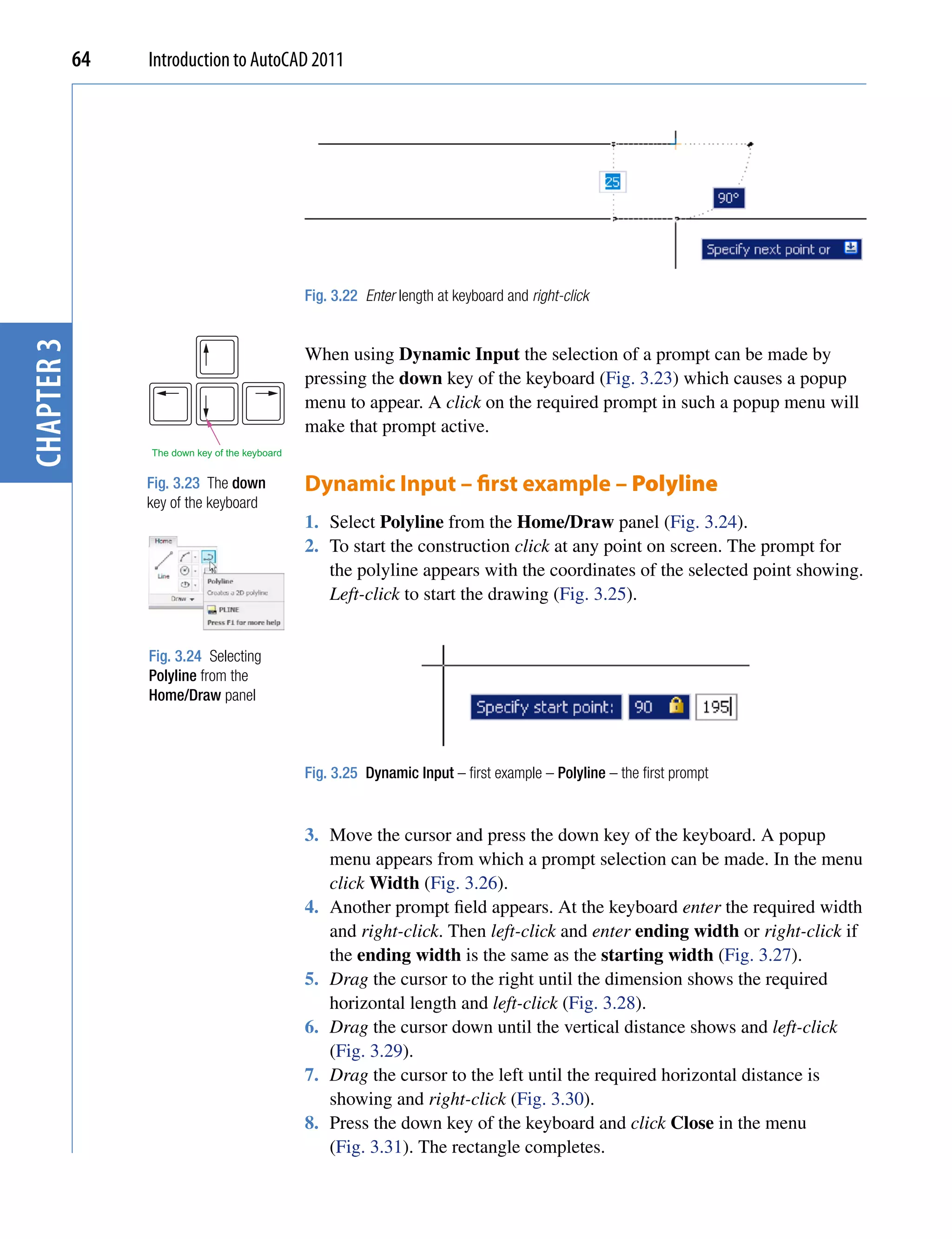
5. Repeat with pline 5 and enter j in response to the prompt line:](https://image.slidesharecdn.com/introductiontoautocad2011-100614022653-phpapp02/75/Introduction-to-AutoCad-2011-71-2048.jpg)
![Draw tools, Object Snap and Dynamic Input 73
Enter an option [Open/Join/Width/Edit vertex/Fit/
Spline/Decurve/Ltype gen/Undo]: enter j
The result is shown in pline 6.
The resulting examples are shown in Fig. 3.42.
1 2 3
chapter 3
Pline 120�80
Pedit to Width�2 Pedit to Width�10
of Width�0
4 5 6
Pedit using the Pedit drawing 5
Pline with open side
Spline prompt using Close
Fig. 3.42 Examples – Polyline Edit
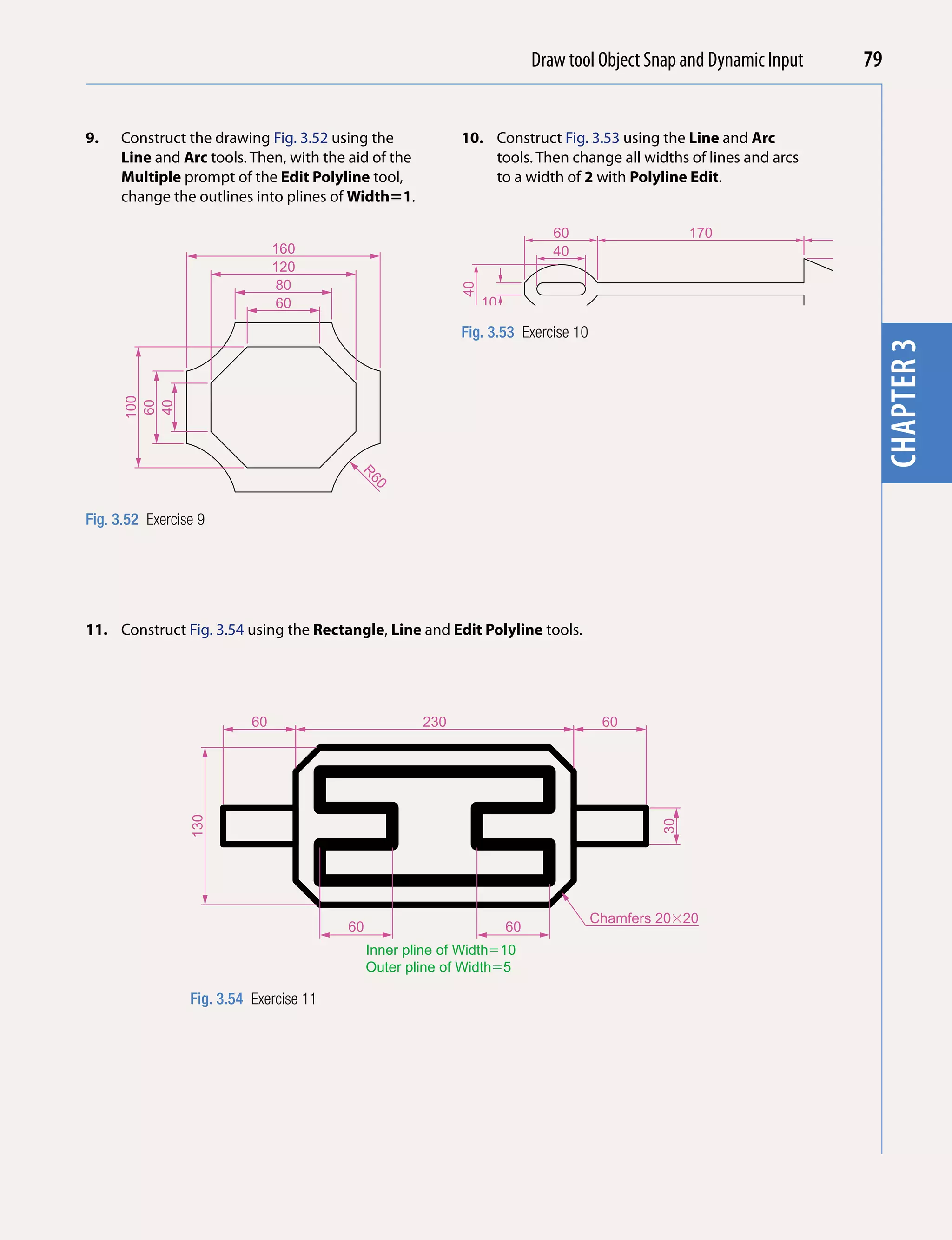
Example – Multiple Polyline Edit (Fig. 3.43)
1. With the Polyline tool construct the left-hand outlines of Fig. 3.43.
2. Call the Edit Polyline tool. The command line shows:
20 20 60 20 20
15
20
30
80
60
100
30
20
15 After Multiple Pedit
pick Outlines using
Line and Arc to Width=2
Fig. 3.43 Example – Multiple Polyline Edit](https://image.slidesharecdn.com/introductiontoautocad2011-100614022653-phpapp02/75/Introduction-to-AutoCad-2011-72-2048.jpg)
![74 Introduction to AutoCAD 2011
Command: enter pe
PEDIT Select polyline or [Multiple]: m (Multiple)
Select objects: pick any one of the lines or arcs
of the left-hand outlines of Fig. 6.16 1 found
Select objects: pick another line or arc 1 found 2
total
Continue selecting lines and arcs as shown by the
pick boxes of the left-hand drawing of Fig. 3.45
until the command line shows:
chapter 3
Select objects: pick another line or arc 1 found
24 total
Select objects: right-click
[prompts]: w (Width)
Specify new width for all segments: 1.5
Convert Arcs, Lines and Splines to polylines [Yes/
No]? <Y>: right-click
[prompts]: right-click
Command:
The result is shown in the right-hand drawing of Fig. 3.43.
transparent commands
When any tool is in operation it can be interrupted by prefixing the
interrupting command with an apostrophe (’). This is particularly useful
when wishing to zoom when constructing a drawing (see page 82). As an
example when the Line tool is being used:
Command:_line
Specify first point: 100,120
Specify next point: 190,120
Specify next point: enter ’z (Zoom)
>> Specify corner of window or [prompts]: pick
>>>> Specify opposite corner: pick
Resuming line command.
Specify next point:
And so on. The transparent command method can be used with any tool.
the set variable peLLipse
Many of the operations performed in AutoCAD are carried out under
settings of SET VARIABLES. Some of the numerous set variables](https://image.slidesharecdn.com/introductiontoautocad2011-100614022653-phpapp02/75/Introduction-to-AutoCad-2011-73-2048.jpg)
![82 Introduction to AutoCAD 2011
introduction
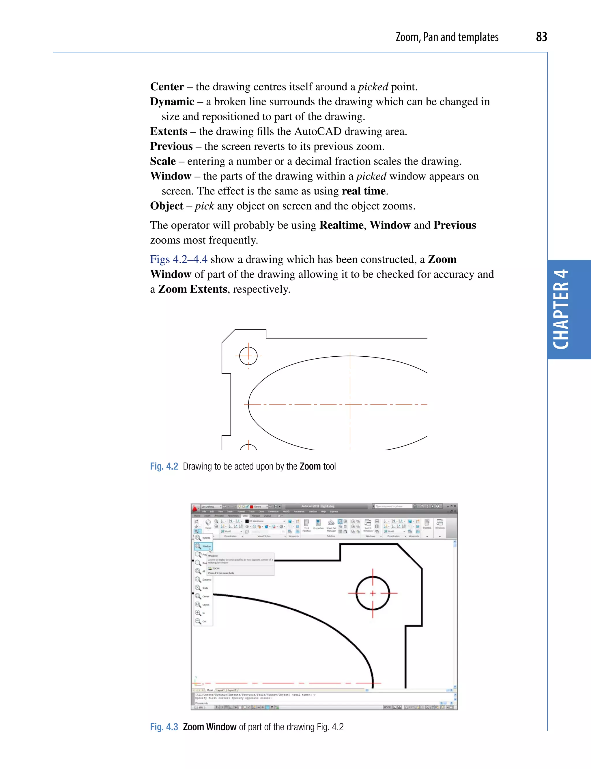
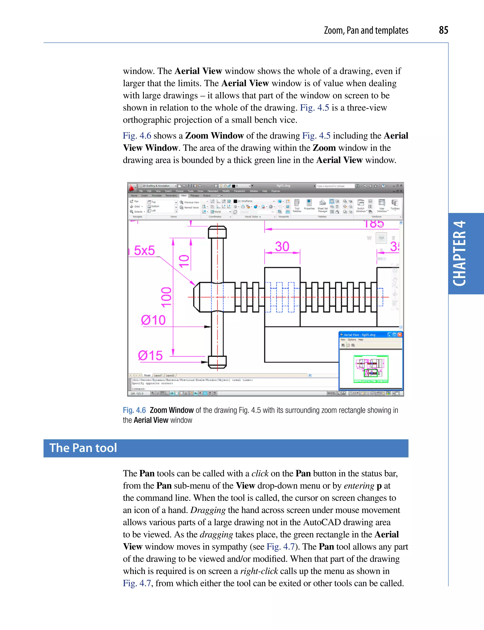
The use of the Zoom tools allows not only the close inspection of the most
minute areas of a drawing in the AutoCAD 2011 drawing area, but also the
accurate construction of very small details in a drawing.
The Zoom tools can be called by selection from the View/Navigate panel
or from the View drop-down menu (Fig. 4.1). However by far the easiest
and quickest method of calling the Zoom is to enter z at the command line
as follows:
Command: enter z right-click
ZOOM Specify corner of window, enter a scale factor
(nX or nXP) or [All/Center/Dynamic/Extents/
chapter 4
Previous/Scale/Window/Object] <real time>:
Fig. 4.1 Calling Zoom – from the Zoom/Navigate panel or from the View drop-down menu
This allows the different zooms:
Realtime – selects parts of a drawing within a window.
All – the screen reverts to the limits of the template.](https://image.slidesharecdn.com/introductiontoautocad2011-100614022653-phpapp02/75/Introduction-to-AutoCad-2011-80-2048.jpg)


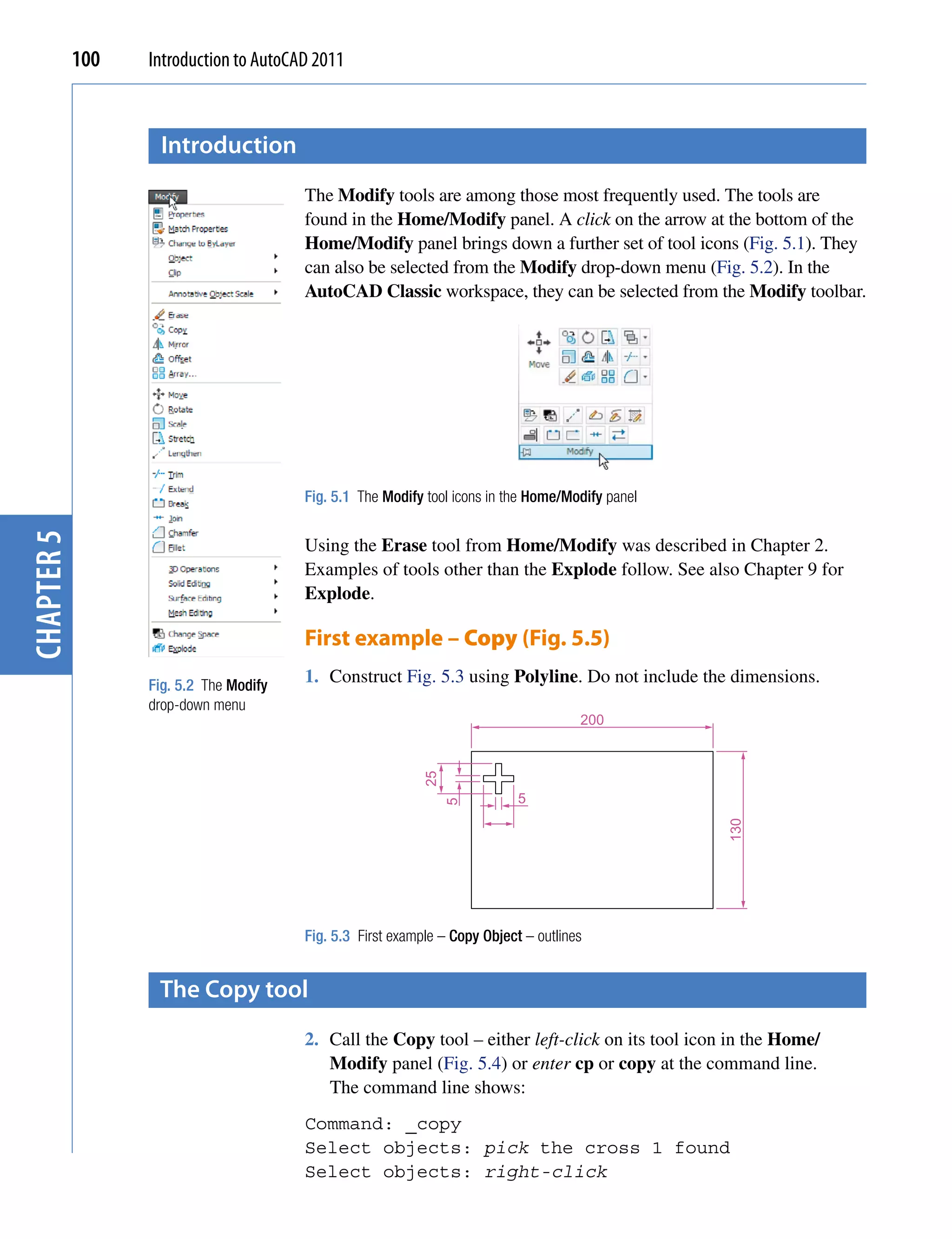
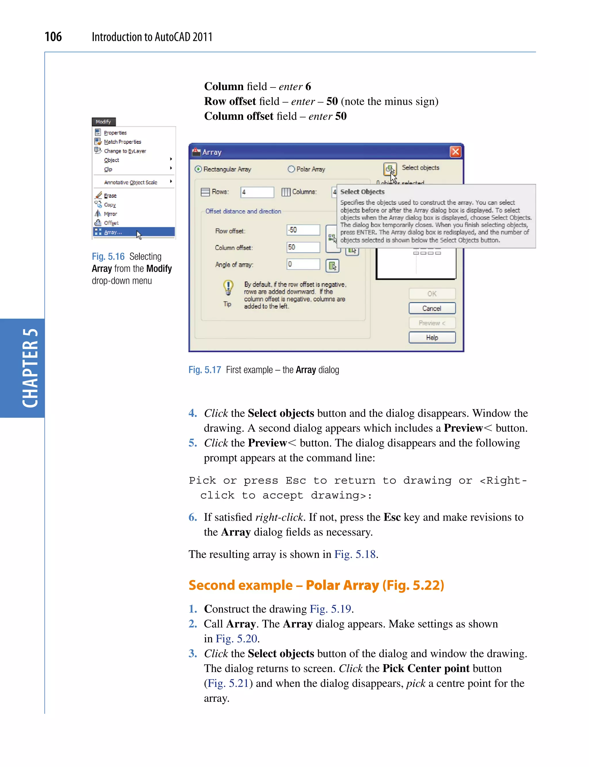
![The Modify tools 101
Current settings: Copy mode = Multiple
Specify base point or [Displacement/mOde]
<Displacement>: pick
Specify second point or [Exit/Undo]: pick
Specify second point or [Exit/Undo] <Exit>:
right-click
Command:
The result is given in Fig. 5.5.
chapter 5
Fig. 5.4 The Copy tool from the Home/Modify panel
base point
second point
Fig. 5.5 First example – Copy
Second example – Multiple copy (Fig. 5.6)
1. Erase the copied object.
2. Call the Copy tool. The command line shows:
Command: _copy
Select objects: pick the cross 1 found
Select objects: right-click
Current settings: Copy mode = Multiple
Specify base point or [Displacement/mOde]
<Displacement>: pick
Specify second point or <use first point as
displacement>: pick](https://image.slidesharecdn.com/introductiontoautocad2011-100614022653-phpapp02/75/Introduction-to-AutoCad-2011-99-2048.jpg)
![102 Introduction to AutoCAD 2011
Specify second point or [Exit/Undo] <Exit>: pick
Specify second point or [Exit/Undo] <Exit>: pick
Specify second point or [Exit/Undo] <Exit>: e
(Exit)
Command
The result is shown in Fig. 5.6.
base point
second point
Fig. 5.6 Second example – Copy – Multiple copy
chapter 5
the mirror tool
First example – Mirror (Fig. 5.9)
1. Construct the outline Fig. 5.7 using the Line and Arc tools.
30 2. Call the Mirror tool – left-click on its tool icon in the Home/Modify
panel (Fig. 5.8) or from the Modify drop-down menu, or enter mi or
20
mirror at the command line. The command line shows:
35
R35
R5
5
75
R35
35
20
Fig. 5.7 First
example –
Fig. 5.8 The Mirror tool from the Home/Modify panel
Mirror – outline
Command:_mirror
Select objects: pick first corner Specify opposite
corner: pick 7 found
Select objects: right-click
Specify first point of mirror line: pick](https://image.slidesharecdn.com/introductiontoautocad2011-100614022653-phpapp02/75/Introduction-to-AutoCad-2011-100-2048.jpg)
![The Modify tools 103
Specify second point of mirror line: pick
Erase source objects [Yes/No] <N>: right-click
Command:
The result is shown in Fig. 5.9.
Second example – Mirror (Fig. 5.10)
1. Construct the outline shown in the dimensioned polyline in the upper
drawing of Fig. 5.10.
2. Call Mirror and using the tool three times complete the given outline.
The two points shown in Fig. 5.10 are to mirror the right-hand side of
the outline.
first corner first point of
mirror line
chapter 5
Result of
the mirror
operation
second point
of mirror line
opposite corner
Fig. 5.9 First example – Mirror
1 7 1
1−"
8 3−"
8 1−"
8
−"
5
8
first point of
mirror line
second point
of mirror line
Fig. 5.10 Second example – Mirror](https://image.slidesharecdn.com/introductiontoautocad2011-100614022653-phpapp02/75/Introduction-to-AutoCad-2011-101-2048.jpg)
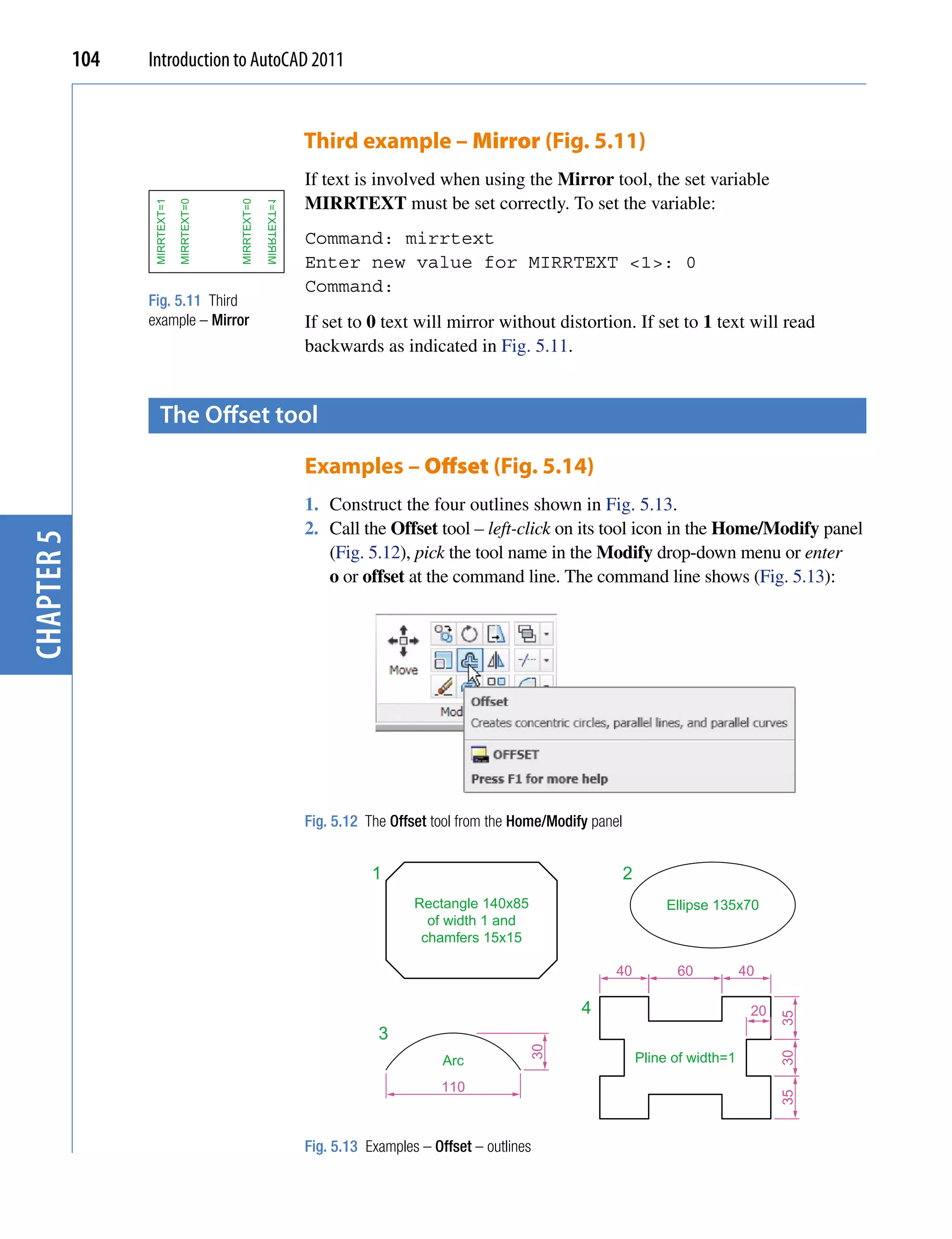
![The Modify tools 105
Command:_offset
Current settings: Erase source = No
Layer=Source OFFSETGAPTYPE=0
Specify offset distance or [Through/Erase/Layer]
<Through>: 10
Select object to offset or [Exit/Undo]
<Exit>: pick drawing 1
Specify point on side to offset or [Exit/Multiple/
Undo] <Exit>: pick inside the rectangle
Select object to offset or [Exit/Undo]
<Exit>: e (Exit)
Command:
3. Repeat for drawings 2, 3 and 4 in Fig. 5.12 as shown in Fig. 5.14.
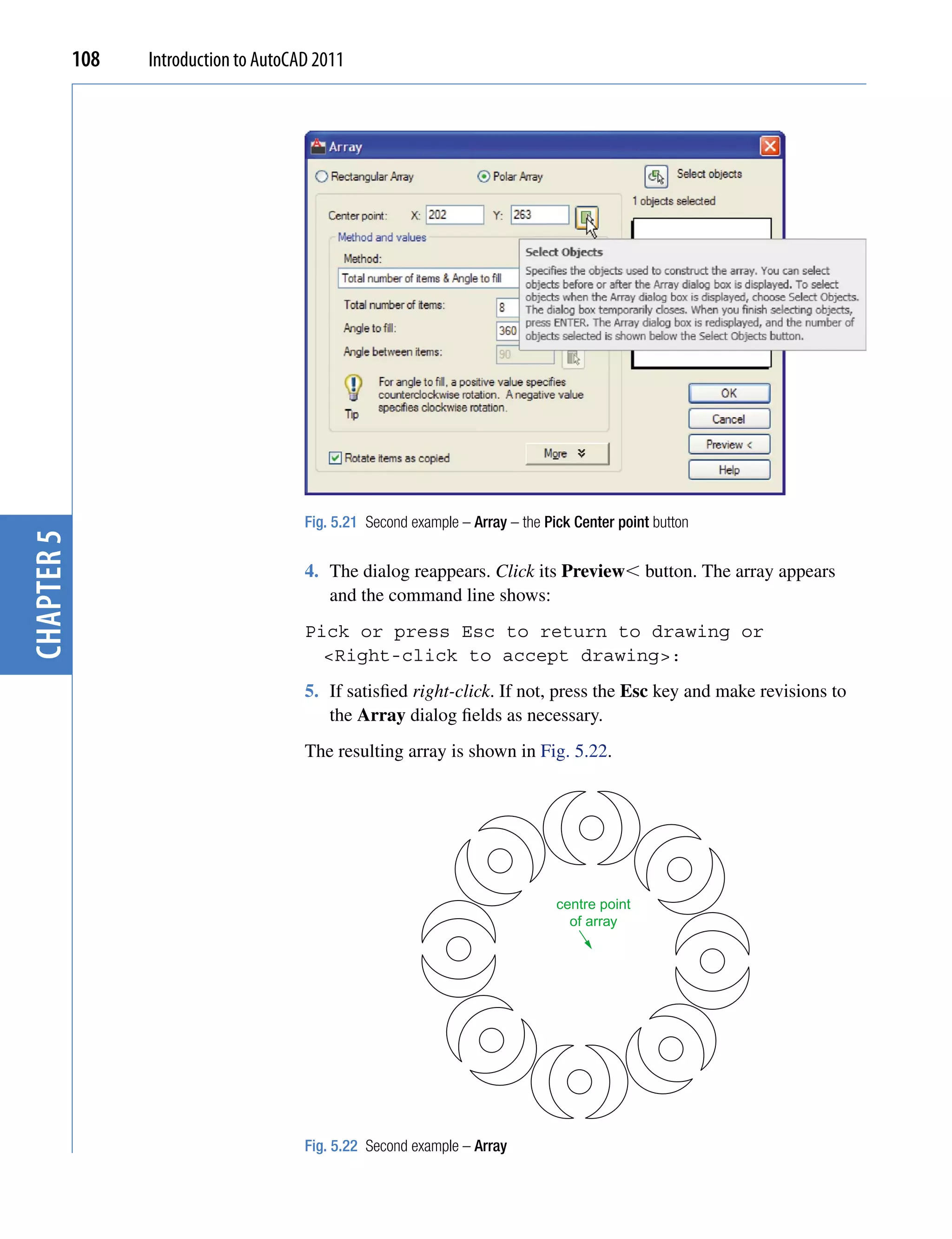
Arrays can be in either a Rectangular form or a Polar form as shown in
the examples below.
chapter 5
Offset 3 times by 5
Offset by 10
Offset inside
and outside
by 7.5
Offset twice by 15
Fig. 5.14 Examples – Offset
the Array tool
First example – Rectangular Array (Fig. 5.17)
40
10 1. Construct the drawing Fig. 5.15.
10
2. Call the Array tool – either click Array in the Modify drop-down
menu (Fig. 5.16), from the Home/Modify panel, or enter ar or array at
40
Ø10
the command line. The Array dialog appears (Fig. 5.17).
3. Make settings in the dialog:
Fig. 5.15 First
example – Array – Rectangular Array radio button set on (dot in button)
drawing to be arrayed Row field – enter 5](https://image.slidesharecdn.com/introductiontoautocad2011-100614022653-phpapp02/75/Introduction-to-AutoCad-2011-103-2048.jpg)
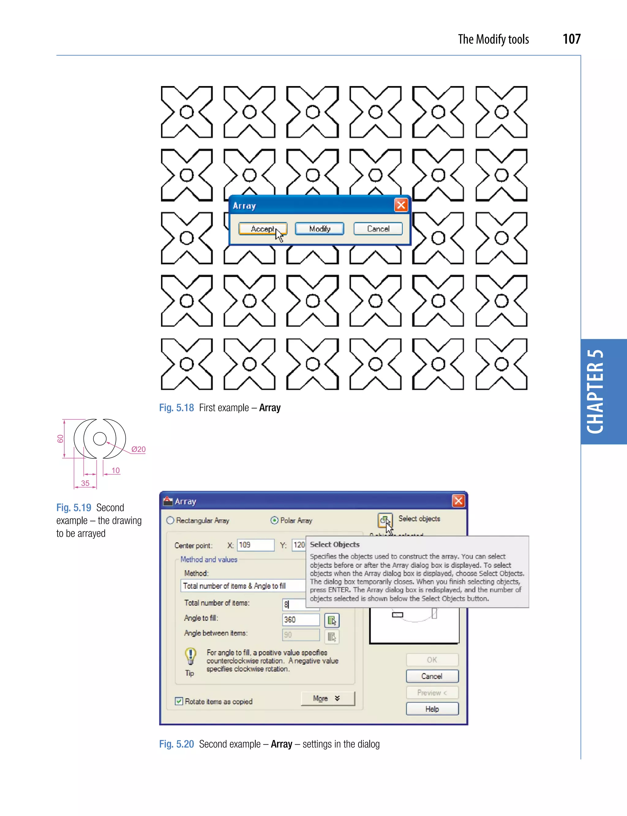
![The Modify tools 109
the move tool
Example – Move (Fig. 5.25)
1. Construct the drawing Fig. 5.23.
Rectangle 190x50. Chafers 10x10
All edges are 5
Fig. 5.23 Example – Move – drawing
2. Call Move – click the Move tool icon in the Home/Modify panel
(Fig. 5.24), pick Move from the Modify drop-down menu or enter m or
chapter 5
move at the command line, which shows:
Fig. 5.24 The Move tool from the Home/Modify panel
Command:_move
Select objects: pick the middle shape in the
drawing 1 found
Select objects: right-click
Specify base point or [Displacement]
<Displacement>: pick
Specify second point or <use first point as
displacement>: pick
Command:
The result is given in Fig. 5.25.](https://image.slidesharecdn.com/introductiontoautocad2011-100614022653-phpapp02/75/Introduction-to-AutoCad-2011-107-2048.jpg)
![110 Introduction to AutoCAD 2011
object which has
been moved
base point second point
Fig. 5.25 Example – Move
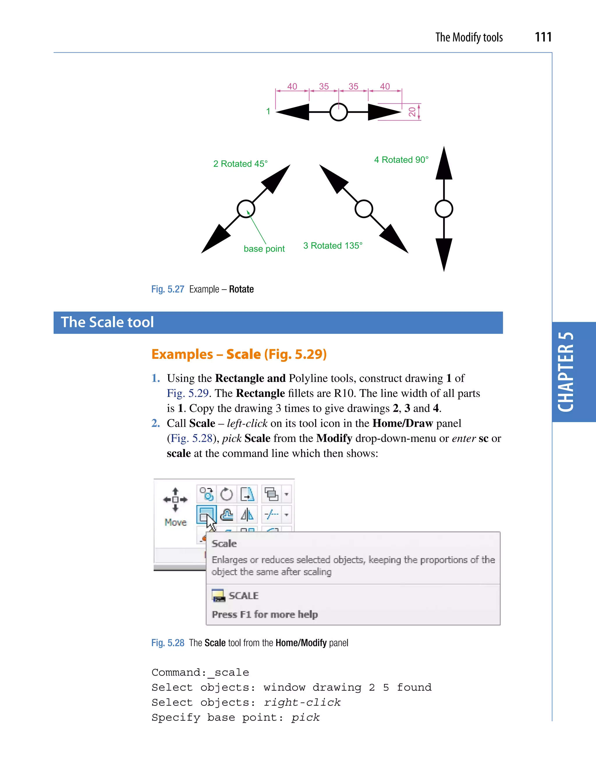
the rotate tool
When using the Rotate tool remember the default rotation of objects
within AutoCAD 2011 is counterclockwise (anticlockwise).
Example – Rotate (Fig. 5.27)
1. Construct drawing 1 of Fig. 5.27 with Polyline. Copy the drawing 1
chapter 5
three times (Fig. 5.27).
2. Call Rotate – left-click on its tool icon in the Home/Modify panel
(Fig. 5.26), pick Rotate from the Modify drop-down menu or enter ro
or rotate at the command line. The command line shows: and the first
copy rotates through the specified angle.
Fig. 5.26 The Rotate tool icon from the Home/Modify panel
Command:_rotate
Current positive angle in UCS:
ANGDIR = counterclockwise ANGBASE=0
Select objects: window the drawing 3 found
Select objects: right-click
Specify base point: pick
Specify rotation angle or [Copy/Reference] <0>: 45
Command:
3. Repeat for drawings 3 and 4 rotating as shown in Fig. 5.27.](https://image.slidesharecdn.com/introductiontoautocad2011-100614022653-phpapp02/75/Introduction-to-AutoCad-2011-108-2048.jpg)
![112 Introduction to AutoCAD 2011
Specify scale factor or [Copy/Reference]
<1>: 0.75
Command:
3. Repeat for the other two drawings 3 and 4 scaling to the scales given
with the drawings.
The results are shown in Fig. 5.29.
3 1 3
1−"
8 3−"
8 −"
4
2
1
1−"
3
8
5
−" Scaled 1.5
8
3 4
Scaled 0.75
chapter 5
Scaled 1.75
base point
Fig. 5.29 Examples – Scale
the trim tool
This tool is one which will be frequent use when constructing drawings.
First example – Trim (Fig. 5.31)
1. Construct the drawing Original drawing in Fig. 5.31.
2. Call Trim – either left-click on its tool icon in the Home/Modify panel
(Fig. 5.30), pick Trim from the Modify drop-down menu or enter tr or
trim at the command line, which then shows:
Fig. 5.30 The Trim tool icon from the Home/Modify panel](https://image.slidesharecdn.com/introductiontoautocad2011-100614022653-phpapp02/75/Introduction-to-AutoCad-2011-110-2048.jpg)
![The Modify tools 113
Command:_trim
Current settings: Projection UCS. Edge = Extend
Select cutting edges . . . .
Select objects or <select all>: pick the left-hand
circle 1 found
Select objects: right-click
Select objects to trim or shift-select to extend
or [Fence/Project/Crossing/Edge/eRase//Undo]:
pick one of the objects
Select objects to trim or shift-select to extend
or
[Fence/Crossing/Project/Edge/eRase/Undo: pick the
second of the objects
Select objects to trim or shift-select to extend
or [Project/Edge/Undo]: right-click
Command:
3. This completes the First stage as shown in Fig. 5.31. Repeat the Trim
chapter 5
sequence for the Second stage.
4. The Third stage drawing of Fig. 5.31 shows the result of the trims at
the left-hand end of the drawing.
5. Repeat for the right-hand end. The final result is shown in the drawing
labelled Result in Fig. 5.31.
100
R20 R15
R15 R10
20
cutting edges Original drawing
objects to trim
cutting edges
First stage Second stage Third stage
Result
Fig. 5.31 First example – Trim](https://image.slidesharecdn.com/introductiontoautocad2011-100614022653-phpapp02/75/Introduction-to-AutoCad-2011-111-2048.jpg)
![114 Introduction to AutoCAD 2011
Second example – Trim (Fig. 5.32)
1. Construct the left-hand drawing of Fig. 5.32.
2. Call Trim. The command line shows:
Command:_trim
Current settings: Projection UCS. Edge = Extend
Select cutting edges . . .
Select objects or <select all>: pick the left-hand
arc 1 found
Select objects: right-click
Select objects to trim or shift-select to extend
or [Fence/Crossing/Project/Edge/eRase/Undo]: e
(Edge)
Enter an implied edge extension mode [Extend/No
extend] <No extend>: e (Extend)
Select objects to trim: pick
Select objects to trim: pick
chapter 5
Select objects to trim: right-click
Command:
3. Repeat for the other required trims. The result is given in Fig. 5.32.
120
80
cutting edges
100
Result
objects to trim
Fig. 5.32 Second example – Trim
the stretch tool
Examples – Stretch (Fig. 5.34)
As its name implies the Stretch tool is for stretching drawings or parts
of drawings. The action of the tool prevents it from altering the shape of](https://image.slidesharecdn.com/introductiontoautocad2011-100614022653-phpapp02/75/Introduction-to-AutoCad-2011-112-2048.jpg)
![The Modify tools 115
circles in any way. Only crossing or polygonal windows can be used to
determine the part of a drawing which is to be stretched.
1. Construct the drawing labelled Original in Fig. 5.34, but do not include
the dimensions. Use the Circle, Arc, Trim and Polyline Edit tools.
The resulting outlines are plines of width 1. With the Copy tool
make two copies of the drawing.
Note
In each of the three examples in Fig. 5.34, the broken lines represent the
crossing windows required when Stretch is used.
2. Call the Stretch tool – either click on its tool icon in the Home/Modify
panel (Fig. 5.33), pick its name in the Modify drop-down menu or enter
s or stretch at the command line, which shows.
chapter 5
Fig. 5.33 The Stretch tool icon from the Home/Modify panel
Command:_stretch
Select objects to stretch by crossing-window
or crossing-polygon. . .
Select objects:enter c right-click
Specify first corner: pick Specify opposite
corner: pick 1 found
Select objects: right-click
Specify base point or [Displacement]
<Displacement>: pick beginning of arrow
Specify second point of displacement or <use first
point as displacement>: drag in the direction
of the arrow to the required second point and
right-click
Command:](https://image.slidesharecdn.com/introductiontoautocad2011-100614022653-phpapp02/75/Introduction-to-AutoCad-2011-113-2048.jpg)
![116 Introduction to AutoCAD 2011
pick corner
120
R20 R10
Original
15
opposite corner
5
5
5
R11
First example
Second example
Third
example
Fig. 5.34 Examples – Stretch
chapter 5
Notes
1. When circles are windowed with the crossing window no stretching
can take place. This is why, in the case of the first example in
Fig. 5.33, when the second point of displacement was picked, there
was no result – the outline did not stretch.
2. Care must be taken when using this tool as unwanted stretching can
occur (Fig. 5.34).
the Break tool
Examples – Break (Fig. 5.36)
1. Construct the rectangle, arc and circle (Fig. 5.36).
2. Call Break – either click on its tool icon in the Home/Modify panel
(Fig. 5.35), click Break in the Modify drop-down menu or enter br or
break at the command line, which shows:
For drawings 1 and 2
Command:_break Select object: pick at the point
Specify second break point or [First point]: pick
Command:](https://image.slidesharecdn.com/introductiontoautocad2011-100614022653-phpapp02/75/Introduction-to-AutoCad-2011-114-2048.jpg)
![The Modify tools 117
Fig. 5.35 The Break tool icon from the Home/Modify panel
For drawing 3
chapter 5
Command:_break Select object pick
Specify second break point or [First point]: enter
f right-click
Specify first break point: pick
Specify second break point: pick
Command:
The results are shown in Fig. 5.36.
1
Select
Result
second break
point
2
Result
second point
3 Select
Result
first point
Fig. 5.36 Examples – Break](https://image.slidesharecdn.com/introductiontoautocad2011-100614022653-phpapp02/75/Introduction-to-AutoCad-2011-115-2048.jpg)
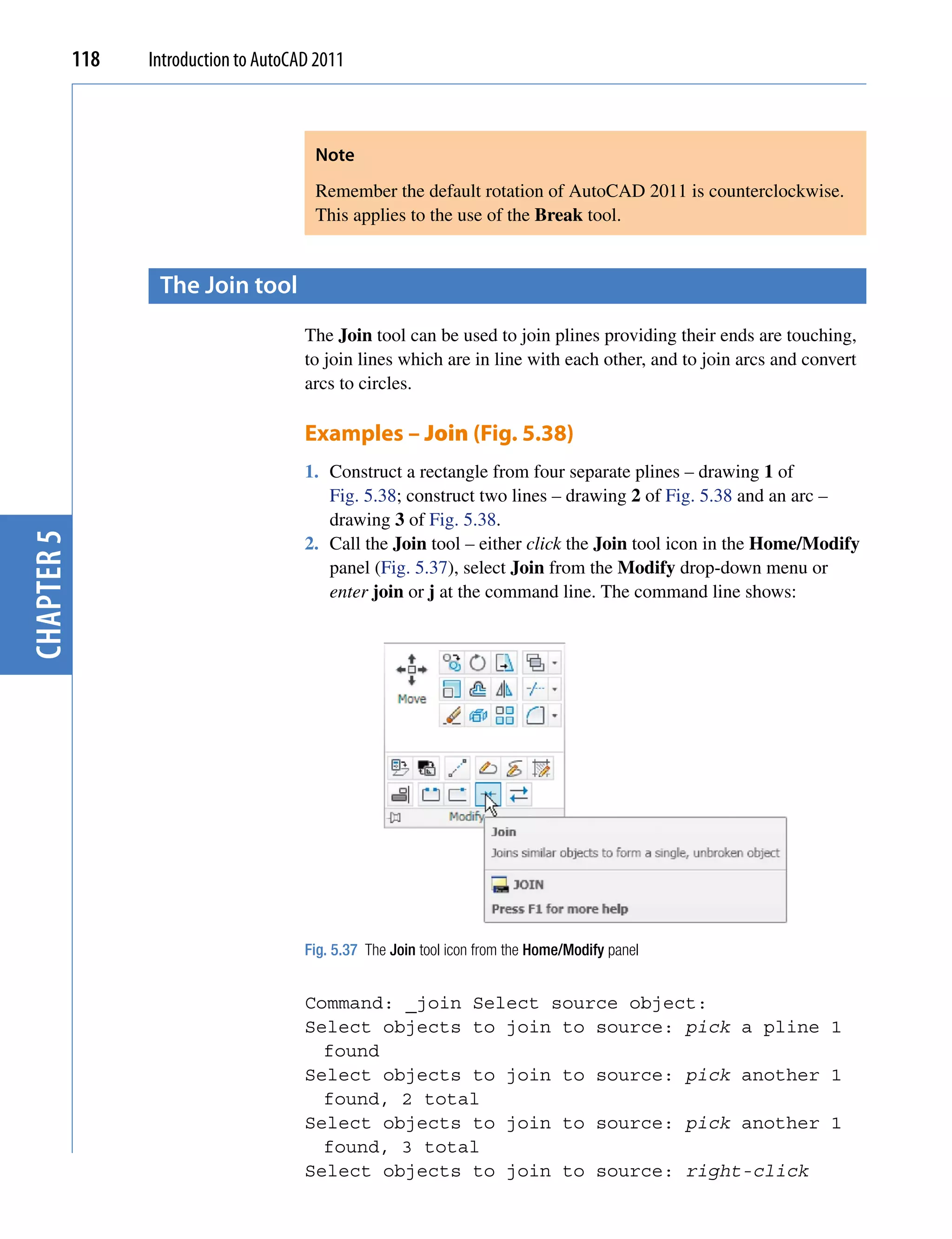
![The Modify tools 119
3 segments added to polyline
Command: right-click
JOIN Select source object: pick one of the lines
Select lines to join to source: pick the other 1
found
Select lines to join to source: right-click
1 line joined to source
Command: right-click
JOIN Select source object: pick the arc
Select arcs to join to source or [cLose]: enter l
right-click
Arc converted to a circle.
Command:
The results are shown in Fig. 5.38.
chapter 5
1 4 separate plines Result 1
a closed polyline
2
Result 2
3
Result 3
Fig. 5.38 Examples – Join
the extend tool
Examples – Extend (Fig. 5.40)
1. Construct plines and a circle as shown in the left-hand drawings of Fig.
5.40.
2. Call Extend – either click the Extend tool icon in the Home/Modify
panel (Fig. 5.39), pick Extend from the Modify drop-down menu or
enter ex or extend at the command line which then shows:
Command:_extend
Current settings: Projection=UCS Edge=Extend
Select boundary edges . . .](https://image.slidesharecdn.com/introductiontoautocad2011-100614022653-phpapp02/75/Introduction-to-AutoCad-2011-117-2048.jpg)
![120 Introduction to AutoCAD 2011
Select objects or <select all>: pick 1 found
Select objects: right-click
Select object to extend or shift-select to trim
or[Fence/Crossing/Project/Edge/Undo]: pick
Repeat for each object to be extended. Then:
Select object to extend or shift-select to trim or
[Fence/Crossing/Project/Edge/Undo]: right-click
Command:
The results are shown in Fig. 5.40.
chapter 5
Fig. 5.39 The Extend tool icon from the Home/Modify panel
objects to
extend
boundary edge Results
objects to
extend
Fig. 5.40 Examples – Extend](https://image.slidesharecdn.com/introductiontoautocad2011-100614022653-phpapp02/75/Introduction-to-AutoCad-2011-118-2048.jpg)
![The Modify tools 121
Note
Observe the similarity of the Extend and No extend prompts with those
of the Trim tool.
the fillet and chamfer tools
These two tools can be called from the Home/Modify panel. There
are similarities in the prompt sequences for these two tools. The major
differences are that only one (Radius) setting is required for a fillet, but
two (Dist1 and Dist2) are required for a chamfer. The basic prompts for
both are:
Fillet
chapter 5
Command:_fillet
Current settings: Mode = TRIM, Radius = 1
Select first object or [Polyline/Radius/Trim/
mUltiple]: enter r (Radius)right-click
Specify fillet radius <1>: 15
Chamfer
Command:_chamfer
(TRIM mode) Current chamfer Dist1 = 1, Dist2 = 1
Select first line or [Undo/Polyline/Distance/Angle/
Trim/mEthod/Multiple]: enter d (Distance)
right-click
Specify first chamfer distance <1>: 10
Specify second chamfer distance <10>: right-click
Examples – Fillet (Fig. 5.42)
1. Construct three rectangles 100 by 60 using either the Line or the
Polyline tool (Fig. 5.42).
2. Call Fillet – click the arrow to the right of the tool icon in the Home/
Modify panel and select Fillet from the menu which appears
(Fig. 5.41), pick Fillet from the Modify drop-down menu or enter f or
fillet at the command line which then shows:
Command:_fillet
Current settings: Mode = TRIM, Radius = 1](https://image.slidesharecdn.com/introductiontoautocad2011-100614022653-phpapp02/75/Introduction-to-AutoCad-2011-119-2048.jpg)
![122 Introduction to AutoCAD 2011
Select first object or [Polyline/Radius/Trim/
mUltiple]: r (Radius)
Specify fillet radius <0>: 15
Select first object or [Undo/Polyline/Radius/Trim/
Multiple]: pick
Select second object or shift-select to apply
corner: pick
Command:
Three examples are given in Fig. 5.42.
chapter 5
Fig. 5.41 Select Fillet from the menu in the Home/Modify panel
Original
rectangle Radius�10
100�60
Radius�15
Radius�20
No trim
Fig. 5.42 Examples – Fillet
Examples – Chamfer (Fig. 5.44)
1. Construct three rectangles 100 by 60 using either the Line or the
Polyline tool.
2. Call Chamfer – click the arrow to the right of the tool icon in the
Home/Modify panel and select Chamfer from the menu which appears](https://image.slidesharecdn.com/introductiontoautocad2011-100614022653-phpapp02/75/Introduction-to-AutoCad-2011-120-2048.jpg)
![The Modify tools 123
(Fig. 5.43), pick Chamfer from the Modify drop-down menu or enter
cha or chamfer at the command line which then shows:
Fig. 5.43 Select Chamfer from the Home/Modify panel
Command:_chamfer
(TRIM mode) Current chamfer Dist1 = 1, Dist2 = 1
Select first line or [Undo/Polyline/Distance/Angle/
chapter 5
Trim/
mEthod/Multiple]: d
Specify first chamfer distance <1>: 10
Specify second chamfer distance <10>: right-click
Select first line or [Undo/Polyline/Distance/Angle/
Trim/mEthod/Multiple]:pick the first line for the
chamfer
Select second line or shift-select to apply
corner: pick
Command:
The result is shown in Fig. 5.44. The other two rectangles are chamfered in
a similar manner except that the No trim prompt is brought into operation
with the bottom left-hand example.
Original
Dist1=10
rectangle
Dist2=10
100x60
Dist1=20
Dist1=10
Dist2=20
Dist2=15
No trim
Fig. 5.44 Examples – Chamfer](https://image.slidesharecdn.com/introductiontoautocad2011-100614022653-phpapp02/75/Introduction-to-AutoCad-2011-121-2048.jpg)


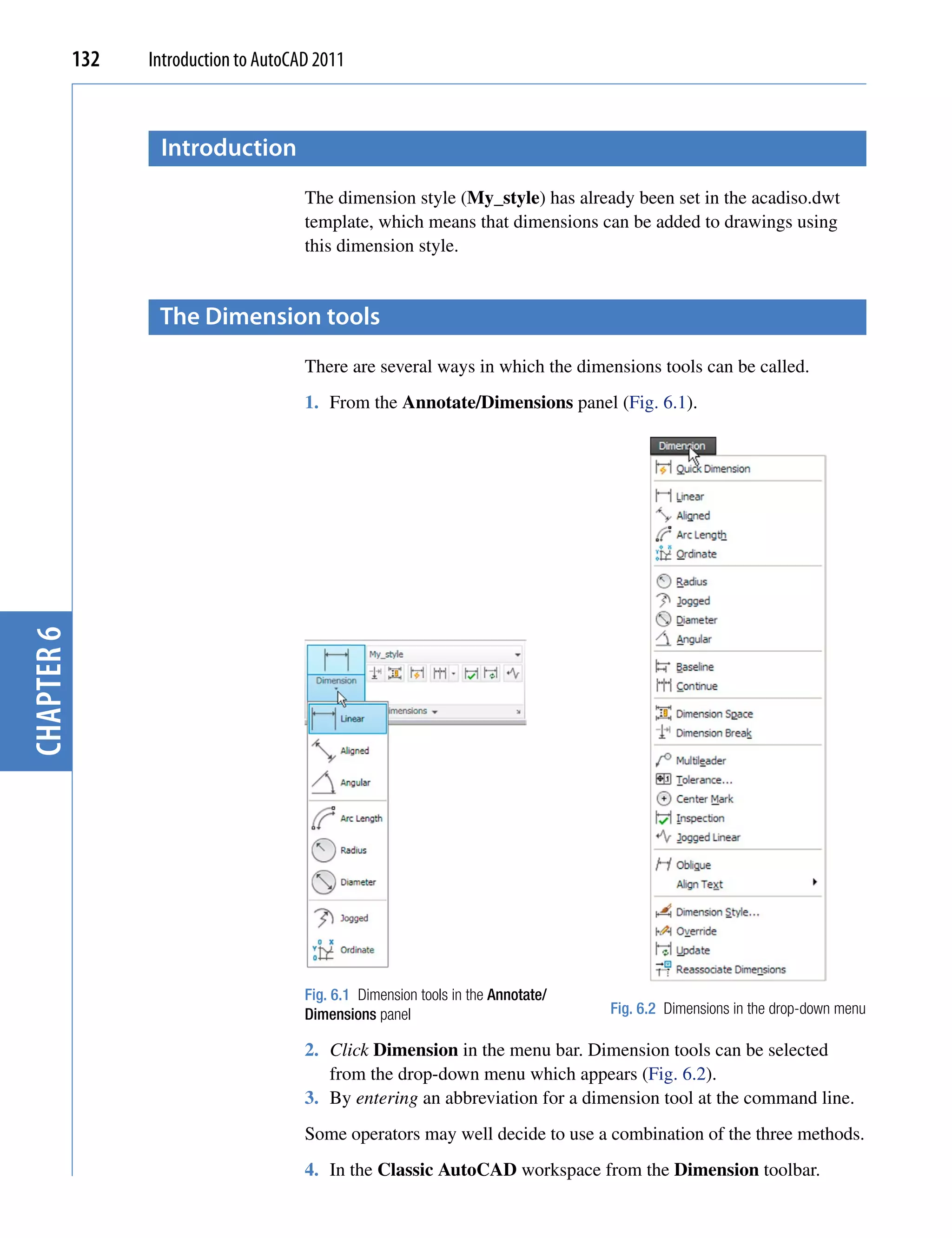
![Dimensions and Text 133
Note
In general, in this book dimensions are shown in drawings in the Metric
style – mainly in millimetres, but some will be shown in Imperial
style – in inches. To see how to set a drawing template for Imperial
dimensioning see Chapter 4 (page 95).
Adding dimensions using these tools
First example – Linear Dimension (Fig. 6.4)
1. Construct a rectangle 180 110 using the Polyline tool.
2. Make the Dimensions layer current from the Home/Layers panel
(Fig. 6.3).
chapter 6
Fig. 6.3 The Home/Layers panel – making Dimensions layer current
3. Click the Linear tool icon in the Annotate/Dimension panel (Fig. 6.1).
The command line shows:
Command: _dimlinear
Specify first extension line origin or <select
object>: pick
Specify second extension line origin: pick
Specify dimension line location or [Mtext/
Text/Angle/Horizontal/Vertical/Rotated] pick
:
Dimension text = 180
Command:
Fig. 6.4 shows the 180 dimension. Follow exactly the same procedure for
the 110 dimension.](https://image.slidesharecdn.com/introductiontoautocad2011-100614022653-phpapp02/75/Introduction-to-AutoCad-2011-130-2048.jpg)
![134 Introduction to AutoCAD 2011
Dimension line location
First Second
extension extension
line 180 line
110
Fig. 6.4 First example – Linear dimension
Notes
1. If necessary use Osnaps to locate the extension line locations.
2. At the prompt:
Specify first extension line origin or [select
object]
:
Also allows the line being dimensioned to be picked.
chapter 6
3. The drop-down menu from the Line tool icon contains the following
tool icons – Angular, Linear, Aligned, Arc Length, Radius,
Diameter, Jog Line and Ordinate. Refer to Fig. 6.1 when working
through the examples below. Note – when a tool is chosen from this
menu, the icon in the panel changes to the selected tool icon.
Second example – Aligned Dimension (Fig. 6.5)
1. Construct the outline Fig. 6.5 using the Line tool.
170
99
13
9
50
170
Fig. 6.5 Second example – Aligned dimension](https://image.slidesharecdn.com/introductiontoautocad2011-100614022653-phpapp02/75/Introduction-to-AutoCad-2011-131-2048.jpg)
![Dimensions and Text 135
2. Make the Dimensions layer current (Home/Layers panel).
3. Left-click the Aligned tool icon (see Fig. 6.1) and dimension the
outline. The prompts and replies are similar to the first example.
Third example – Radius Dimension (Fig. 6.6)
1. Construct the outline Fig. 6.5 using the Line and Fillet tools.
2. Make the Dimensions layer current (Home/Layers panel).
3. Left-click the Radius tool icon (see Fig. 6.1). The command line shows:
Command:_dimradius
Select arc or circle: pick one of the arcs
Dimension text = 30
Specify dimension line location or [Mtext/Text/
Angle] pick
:
Command:
4. Continue dimensioning the outline as shown in Fig. 6.6.
190
R30 R20
chapter 6
100
Fig. 6.6 Third example – Radius dimension
Notes
1. At the prompt:
[Mtext/Text/Angle] :
If a t (Text) is entered, another number can be entered, but remember
if the dimension is a radius the letter R must be entered as a prefix to
the new number.
2. If the response is a (Angle), and an angle number is entered the text
for the dimension will appear at an angle.
3. If the response is m (Mtext) the Text Formatting dialog appears
together with a box in which new text can be entered. See page 147.
4. Dimensions added to a drawing using other tools from the Annotate/
Dimensions panel should be practised.](https://image.slidesharecdn.com/introductiontoautocad2011-100614022653-phpapp02/75/Introduction-to-AutoCad-2011-132-2048.jpg)
![136 Introduction to AutoCAD 2011
Adding dimensions from the command line
From Figs 6.1 and 6.2 it will be seen that there are some dimension tools
which have not been described in examples. Some operators may prefer
entering dimensions from the command line. This involves abbreviations
for the required dimension such as:
For Linear Dimension – hor (horizontal) or ve (vertical);
For Aligned Dimension – al;
For Radius Dimension – ra;
For Diameter Dimension – d;
For Angular Dimension – an;
For Dimension Text Edit – te;
For Quick Leader – l.
And to exit from the dimension commands – e (Exit).
First example – hor and ve (horizontal and
vertical) – Fig. 6.8
1. Construct the outline Fig. 6.7 using the Line tool. Its dimensions are
shown in Fig. 6.8.
chapter 6
Fig. 6.7 First example – outline to dimension
2. Make the Dimensions layer current (Home/Layers panel).
3. At the command line enter dim. The command line will show:
Command: enter dim right-click
Dim: enter hor (horizontal) right-click
Specify first extension line origin or <select
object>: pick
Specify second extension line origin: pick
Non-associative dimension created.
Specify dimension line location or [Mtext/Text/
Angle] pick
:
Enter dimension text <50>: right-click](https://image.slidesharecdn.com/introductiontoautocad2011-100614022653-phpapp02/75/Introduction-to-AutoCad-2011-133-2048.jpg)
![Dimensions and Text 137
Dim: right-click
HORIZONTAL
Specify first extension line origin or <select
object>: pick
Specify second extension line origin: pick
Non-associative dimension created.
Specify dimension line location or [Mtext/Text/
Angle/Horizontal/Vertical/Rotated] pick
:
Enter dimension text <140>: right-click
Dim: right-click
And the 50 and 140 horizontal dimensions are added to the outline.
4. Continue to add the right-hand 50 dimension. Then when the command
line shows:
Dim: enter ve (vertical) right-click
Specify first extension line origin or <select
object>: pick
Specify second extension line origin: pick
Specify dimension line location or [Mtext/Text/
Angle/Horizontal/Vertical/Rotated] pick
:
Dimension text <20>: right-click
chapter 6
Dim: right-click
VERTICAL
Specify first extension line origin or <select
object>: pick
Specify second extension line origin: pick
Specify dimension line location or [Mtext/Text/
Angle/Horizontal/Vertical/Rotated] pick
:
Dimension text <100>: right-click
Dim: enter e (Exit) right-click
Command:
The result is shown in Fig. 6.8.
50 140 50
20
100
Fig. 6.8 First example – horizontal and vertical dimensions](https://image.slidesharecdn.com/introductiontoautocad2011-100614022653-phpapp02/75/Introduction-to-AutoCad-2011-134-2048.jpg)
![138 Introduction to AutoCAD 2011
Second example – an (Angular) – Fig. 6.10
1. Construct the outline Fig. 6.9 – a pline of width 1.
60 60 40
40
45
90
290
Fig. 6.9 Second example – outline for dimensions
2. Make the Dimensions layer current (Home/Layers panel).
3. At the command line:
Command: enter dim right-click
Dim: enter an right-click
Select arc, circle, line or <specify vertex>: pick
chapter 6
Select second line: pick
Specify dimension arc line location or [Mtext/
Text/Angle/Quadrant] pick
:
Enter dimension <90>: right-click
Enter text location (or press ENTER) pick
:
Dim:
And so on to add the other angular dimensions.
The result is given in Fig. 6.10.
60 60
° 135
135 90° °
Select line Select second line
90
290
Fig. 6.10 Second example – an (Angular) dimension](https://image.slidesharecdn.com/introductiontoautocad2011-100614022653-phpapp02/75/Introduction-to-AutoCad-2011-135-2048.jpg)
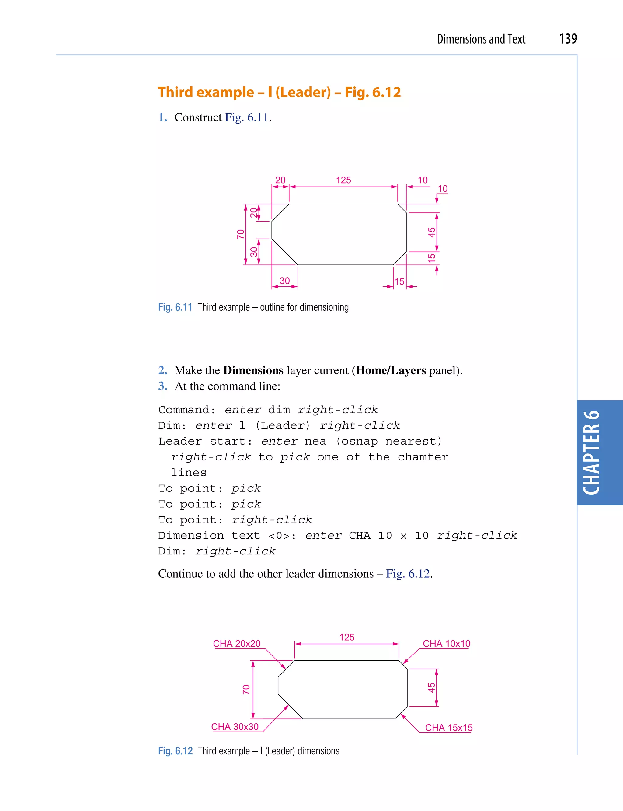
![140 Introduction to AutoCAD 2011
Fourth example – te (dimension text edit) – Fig. 6.14
1. Construct Fig. 6.13.
210
30 20 20
∆20
20 20
130
Polygon
30
Ellipse 30�20
Fig. 6.13 Fourth example – dimensioned drawing
2. Make the Dimensions layer current (Home/Layers panel).
3. At the command line:
Command: enter dim right-click
Dim: enter te (tedit) right-click
chapter 6
Select dimension: pick the dimension to be changed
Specify new location for text or [Left/Right/
Center/Home/Angle] either pick or enter a prompt
:
capital letter
Dim:
The results as given in Fig. 6.14 show dimensions which have been moved.
The 210 dimension changed to the left-hand end of the dimension line, the
130 dimension changed to the left-hand end of the dimension line and the
30 dimension position changed.
210
30 20 20
20 20
∆20
130
Polygon
30
Ellipse 30�20
Fig. 6.14 Fourth example – dimensions amended with tedit](https://image.slidesharecdn.com/introductiontoautocad2011-100614022653-phpapp02/75/Introduction-to-AutoCad-2011-137-2048.jpg)
![Dimensions and Text 141
the Arc Length tool (Fig. 6.15)
1. Construct two arcs of different sizes as in Fig. 6.15.
147
62
213
Fig. 6.15 Examples – Arc Length tool
2. Make the Dimensions layer current (Home/Layers panel).
3. Call the Arc Length tool from the Annotate/Dimensions panel (see
Fig. 6.3) or enter dimarc at the command line. The command line shows:
Command: _dimarc
Select arc or polyline arc segment: pick an arc
Specify arc length dimension location, or [Mtext/
chapter 6
Text/Angle/Partial/Leader] pick a suitable
:
position
Dimension text = 147
Command:
Examples on two arcs are shown in Fig. 6.15.
the Jogged tool (Fig. 6.16)
1. Draw a circle and an arc as indicated in Fig. 6.16.
R60
R49
R60
Fig. 6.16 Examples – the Jogged tool](https://image.slidesharecdn.com/introductiontoautocad2011-100614022653-phpapp02/75/Introduction-to-AutoCad-2011-138-2048.jpg)
![142 Introduction to AutoCAD 2011
2. Make the Dimensions layer current (Home/Layers panel).
3. Call the Jogged tool, either with a left-click on its tool icon in the
Annotation/Dimension panel (see Fig. 6.1) or by entering jog at the
command line. The command line shows:
Command: _dimjogged
Select arc or circle: pick the circle or the
arc
Specify center location override:
pick
Dimension text = 60
Specify dimension line location or [Mtext/Text/
Angle] pick
:
Specify jog location: pick
Command:
The results of placing as jogged dimension on a circle and an arc are
shown in Fig. 6.16.
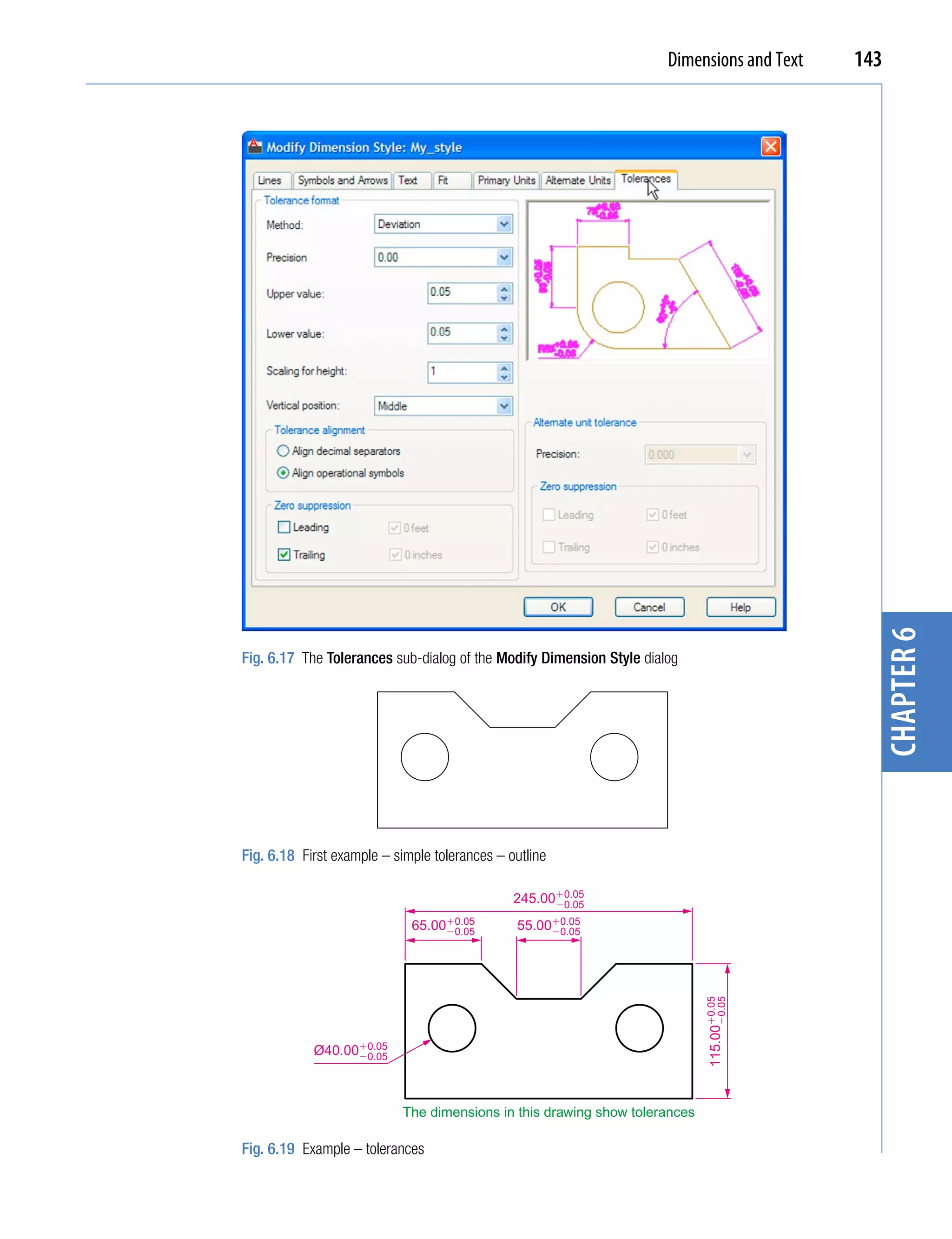
Dimension tolerances
chapter 6
Before simple tolerances can be included with dimensions, new settings
will need to be made in the Dimension Style Manager dialog as
follows:
1. Open the dialog. The quickest way of doing this is to enter d at the
command line followed by a right-click. This opens up the dialog.
2. Click the Modify… button of the dialog, followed by a left-click on
the Primary Units tab and in the resulting sub-dialog make settings
as shown in Fig. 6.17. Note the changes in the preview box of the
dialog.
Example – tolerances (Fig. 6.19)
1. Construct the outline Fig. 6.18.
2. Make the Dimensions layer current (Home/Layers panel).
3. Dimension the drawing using either tools from the Dimension panel
or by entering abbreviations at the command line. Because tolerances
have been set in the Dimension Style Manager dialog (Fig. 6.17), the
toleranced dimensions will automatically be added to the drawing
(Fig. 6.19).](https://image.slidesharecdn.com/introductiontoautocad2011-100614022653-phpapp02/75/Introduction-to-AutoCad-2011-139-2048.jpg)
![144 Introduction to AutoCAD 2011
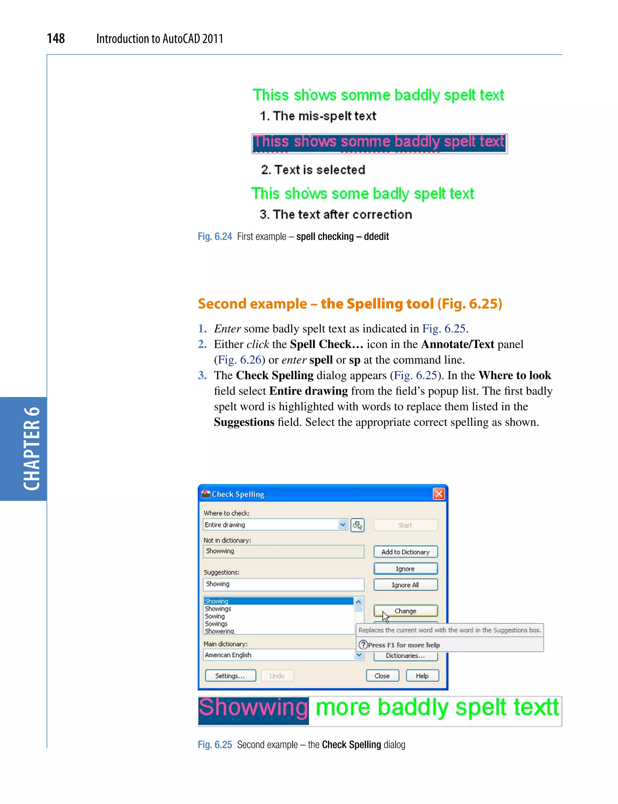
text
There are two main methods of adding text to drawings – Multiline Text
and Single Line Text.
Example – Single Line Text (Fig. 6.19)
1. Open the drawing from the example on tolerances – Fig. 6.19.
2. Make the Text layer current (Home/Layers panel).
3. At the command line enter dt (for Single Line Text) followed by a
right-click:
Command: enter dt right-click
TEXT
Current text style “ARIAL” Text height: 8
Annotative No:
Specify start point of text or [Justify/Style]:
pick
Specify rotation angle of text <0>: right-click
Enter text: enter The dimensions in this drawing
show tolerances press the Return key twice
chapter 6
Command:
The result is given in Fig. 6.19.
Notes
1. When using Dynamic Text the Return key of the keyboard is
pressed when the text has been entered. A right-click does not
work.
2. At the prompt:
Specify start point of text or [Justify/Style]:
enter s (Style) right-click
Enter style name or [?] <ARIAL>: enter ?
right-click
Enter text style(s) to list <*>: right-click
And an AutoCAD Text Window (Fig. 6.20) appears listing all the
styles which have been selected in the Text Style dialog
(see page 145).](https://image.slidesharecdn.com/introductiontoautocad2011-100614022653-phpapp02/75/Introduction-to-AutoCad-2011-141-2048.jpg)
![Dimensions and Text 145
Fig. 6.20 The AutoCAD Text Window
3. In order to select the required text style its name must be entered at
the prompt:
chapter 6
Enter style name or [?] <ARIAL>: enter Romand
right-click
And the text entered will be in the Romand style of height 9. But only
if that style was previously been selected in the Text Style dialog.
4. Fig. 6.21 shows some text styles from the AutoCAD Text Window.
Fig. 6.21 Some text fonts](https://image.slidesharecdn.com/introductiontoautocad2011-100614022653-phpapp02/75/Introduction-to-AutoCad-2011-142-2048.jpg)
![146 Introduction to AutoCAD 2011
5. There are two types of text fonts available in AutoCAD 2011 – the 5.
There are two types of text fonts available in AutoCAD 2011 – the
AutoCAD SHX fonts and the Windows True Type fonts. The
styles shown in Fig. 6.21 are the ITALIC, ROMAND, ROMANS
and STANDARD styles are AutoCAD text fonts. The TIMES and
ARIAL styles are Windows True Type styles. Most of the True
Type fonts can be entered in Bold, Bold Italic, Italic or Regular
styles, but these variations are not possible with the AutoCAD fonts.
6. The Font name popup list of the Text Style dialog shows that a large
number of text styles are available to the AutoCAD 2011 operator.
It is advisable to practise using a variety of these fonts to familiarise
oneself with the text opportunities available with AutoCAD 2011.
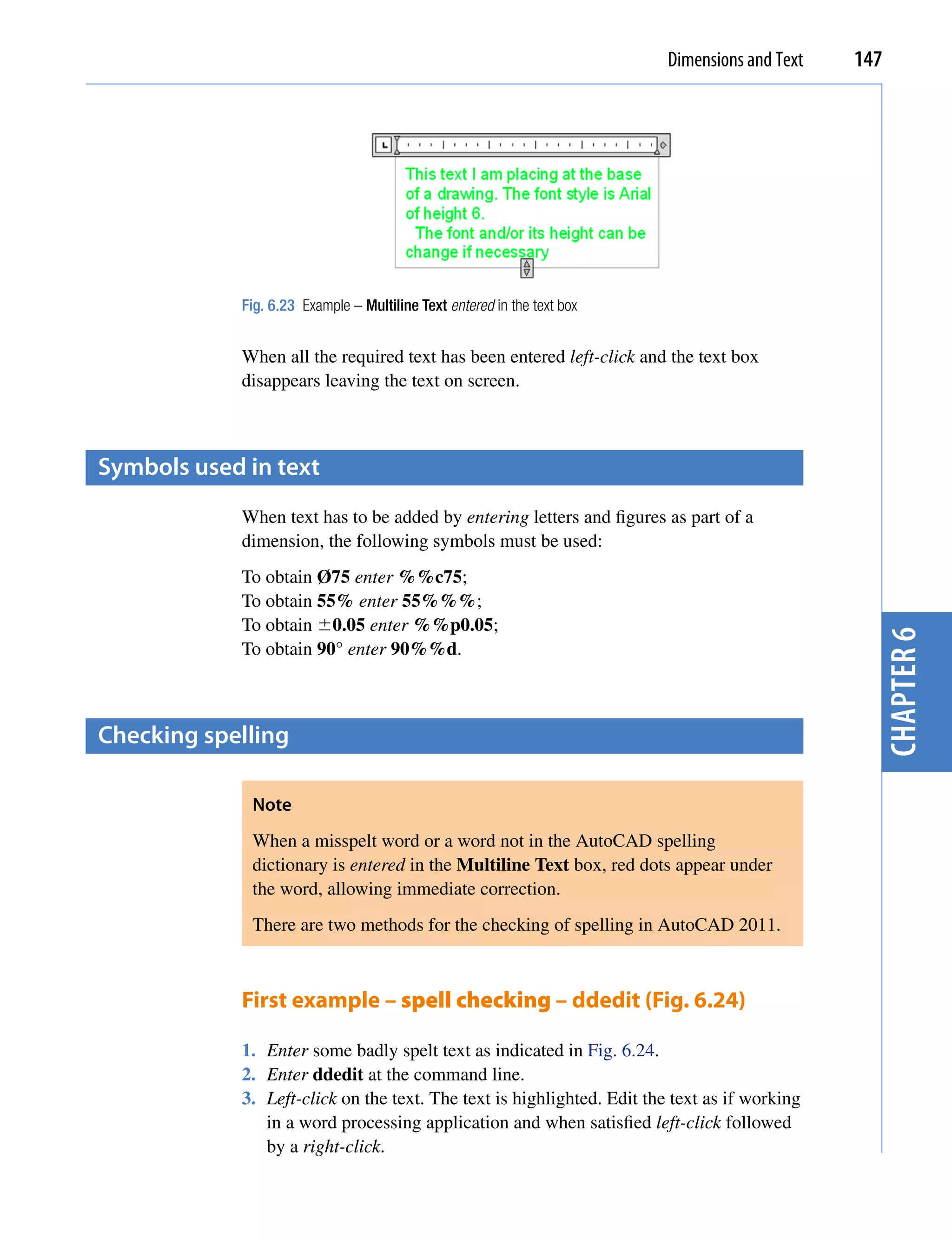
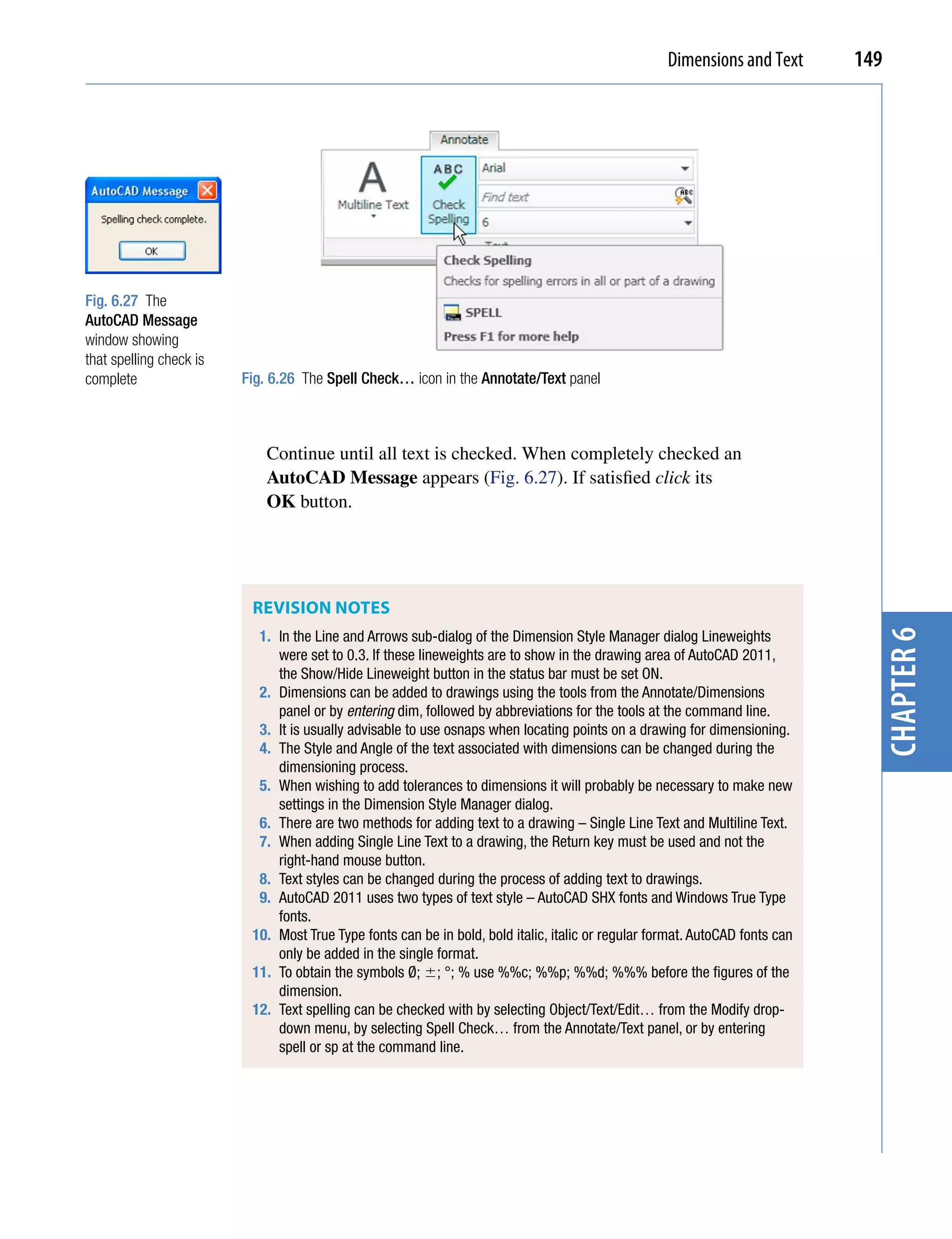
Example – Multiline Text (Fig. 6.23)
1. Make the Text layer current (Home/Layers panel).
2. Either left-click on the Multiline Text tool icon in the Annotate/Text
panel (Fig. 6.22) or enter t at the command line:
chapter 6
Fig. 6.22 Selecting Multiline Text… from the Annotate/Text panel
Command:_mtext
Current text style: “Arial” Text height: 6
Annotative No
Specify first corner: pick
Specify opposite corner or [Height/Justify/Line
spacing/Rotation/Style/Width/Columns] pick
:
As soon as the opposite corner is picked, the Text Formatting box
appears (Fig. 6.23). Text can now be entered as required within the box as
indicated in this illustration.](https://image.slidesharecdn.com/introductiontoautocad2011-100614022653-phpapp02/75/Introduction-to-AutoCad-2011-143-2048.jpg)
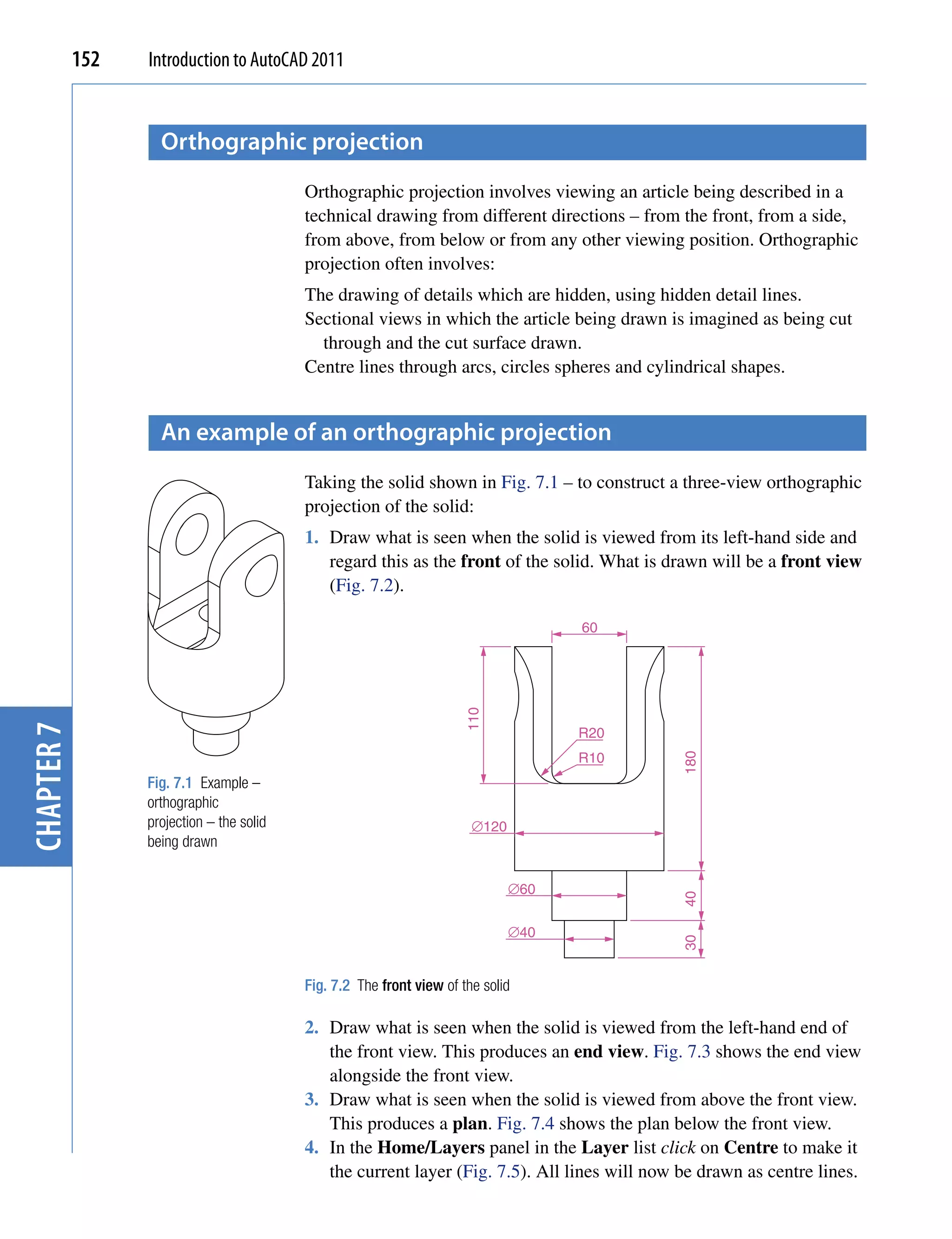
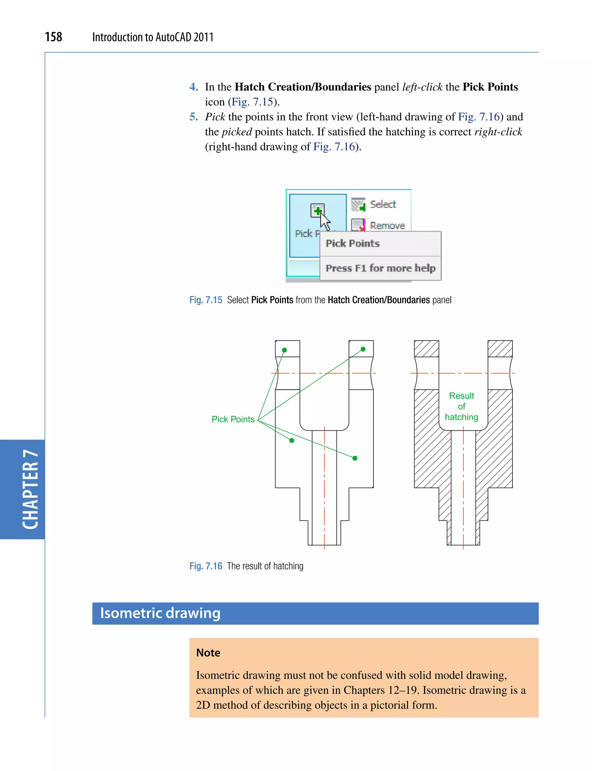
![Orthographic and isometric 159
Setting the AutoCAD window for isometric drawing
To set the AutoCAD 2011 window for the construction of isometric
drawings:
1. At the command line:
Command: enter snap
Specify snap spacing or [On/Off/Aspect/Rotate/
Style/Type] <5>: s (Style)
Enter snap grid style [Standard/Isometric] <S>:
i (Isometric)
Specify vertical spacing <5>: right-click
Command:
And the grid dots in the window assume an isometric pattern as shown in
Fig. 7.17. Note also the cursor hair lines which are at set in an Isometric
Left angle.
chapter 7
Isoplane Top
Fig. 7.17 The AutoCAD grid points set for isometric drawing
Iso ht
pla
ne Rig
Lef lane 2. There are three isometric angles – Isoplane Top, Isoplane Left and
t Isop
Isoplane Right. These can be set by pressing either the F5 function key
or the Ctrl and E keys. Repeated pressing of either of these ‘toggles’
Fig. 7.18 The three between the three settings. Fig. 7.18 is an isometric view showing the
isoplanes three isometric planes.](https://image.slidesharecdn.com/introductiontoautocad2011-100614022653-phpapp02/75/Introduction-to-AutoCad-2011-156-2048.jpg)
![160 Introduction to AutoCAD 2011
The isometric circle
Circles in an isometric drawing show as ellipses. To add an isometric circle
to an isometric drawing, call the Ellipse tool. The command line shows:
Command: _ellipse
Specify axis endpoint of ellipse or [Arc/Center/
Isocircle]: enter i (Isocircle) right-click
Specify center of isocircle: pick or enter
Isoplane Top coordinates
Specify radius of isocircle or [Diameter]: enter a
Iso ht number
pla
ne Rig
Le lane Command:
ft Isop
And the isocircle appears. Its isoplane position is determined by which of
Fig. 7.19 The three the isoplanes is in operation at the time the isocircle was formed. Fig. 7.19
isocircles shows these three isoplanes containing isocircles.
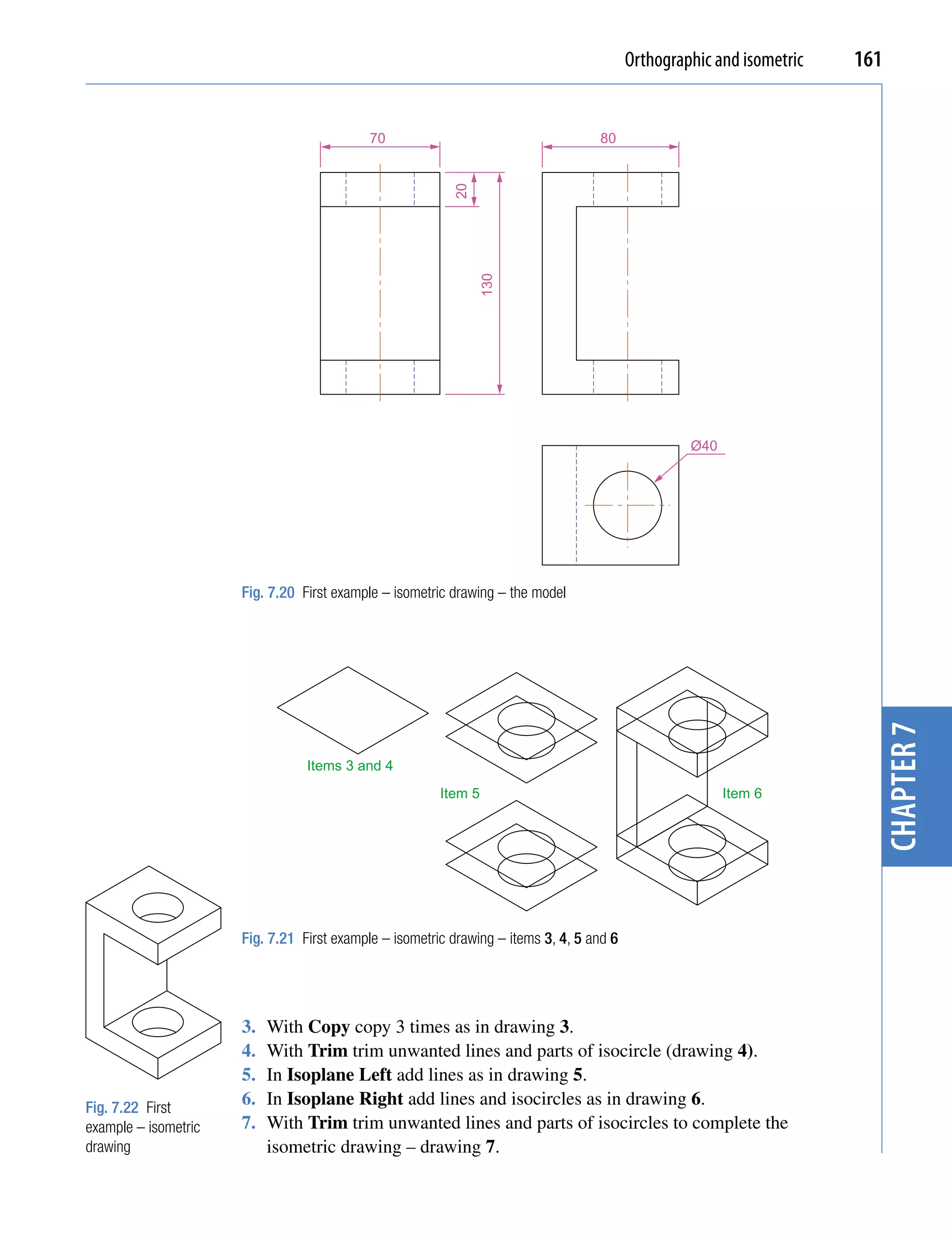
examples of isometric drawings
First example – isometric drawing (Fig. 7.22)
1. This example is to construct an isometric drawing to the details given
in the orthographic projection (Fig. 7.20). Set Snap on (press the F9
function key) and Grid on (F7).
2. Set Snap to Isometric and set the isoplane to Isoplane Top using F5.
chapter 7
3. With Line, construct the outline of the top of the model (Fig. 7.19)
working to the dimensions given in Fig. 7.18.
4. Call Ellipse tool and set to isocircle and add the isocircle of radius 20
centred in its correct position in the outline of the top (Fig. 7.21).
5. Set the isoplane to Isoplane Right and with the Copy tool, copy the top
with its ellipse vertically downwards 3 times as shown in Fig. 7.22.
6. Add lines as shown in Fig. 7.21.
7. Finally using Trim remove unwanted parts of lines and ellipses to
produce Fig. 7.22.
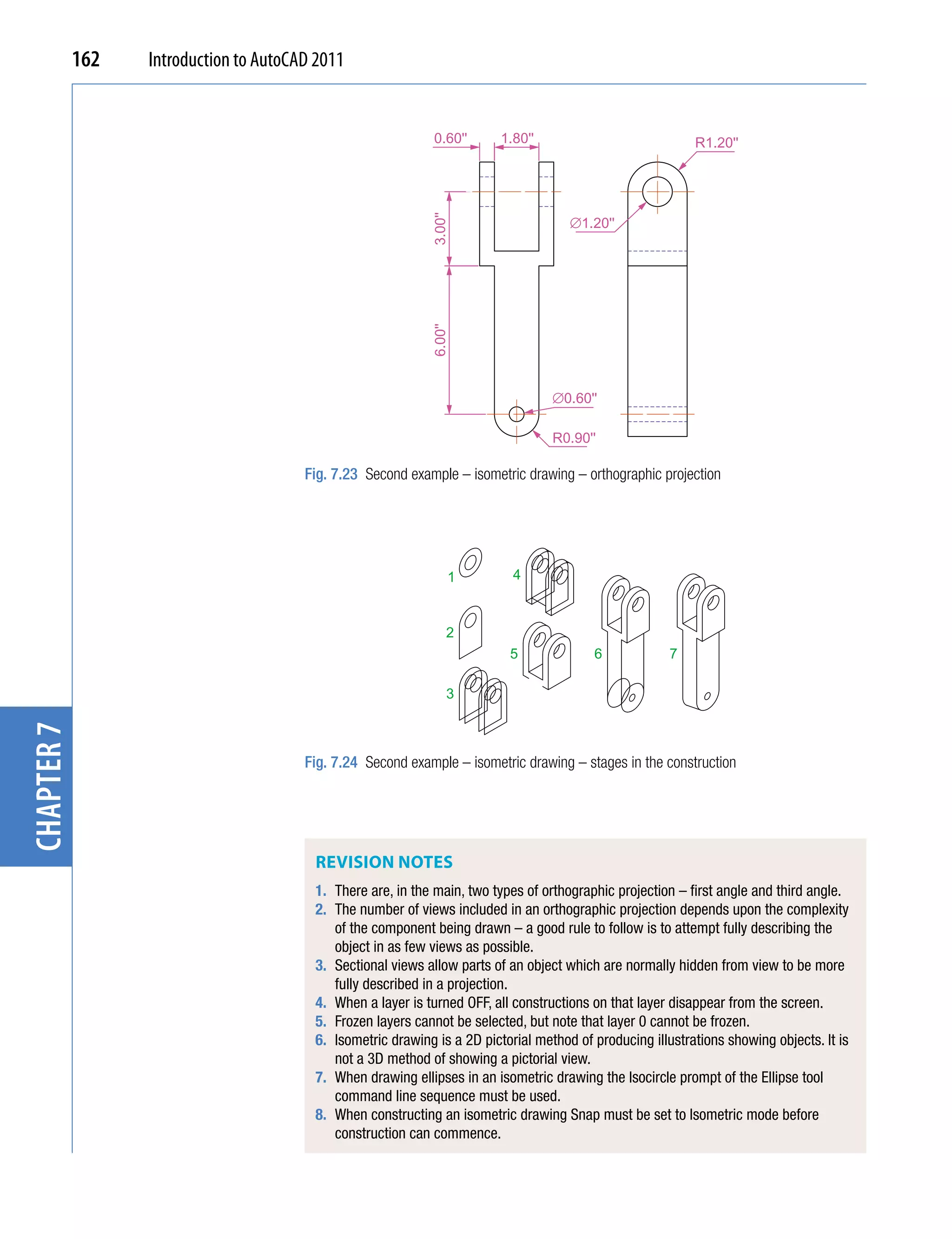
Second example – isometric drawing (Fig. 7.24)
Fig. 7.23 is an orthographic projection of the model of which the isometric
drawing is to be constructed. Fig. 7.24 shows the stages in its construction.
The numbers refer to the items in the list below:
1. In Isoplane Right construct two isocircles of radii 10 and 20.
2. Add lines as in drawing 2 and trim unwanted parts of isocircle.](https://image.slidesharecdn.com/introductiontoautocad2011-100614022653-phpapp02/75/Introduction-to-AutoCad-2011-157-2048.jpg)

![176 Introduction to AutoCAD 2010
2011
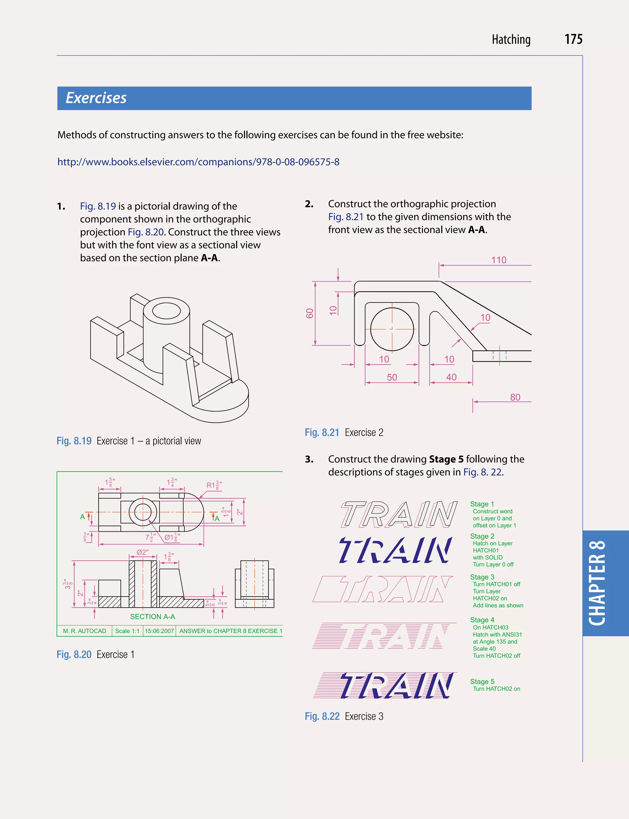
4. Fig. 8.23 is a front view of a car with parts 7. Construct Fig. 8.26 as follows:
chapter 1
hatched. Construct a similar drawing of any
a. On layer Text, construct a circle of
make of car, using hatching to emphasise the
radius 90.
shape.
b. Make layer 0 current.
c. Construct the small drawing to the details
as shown and save as a block with a block
name shape (see Chapter 9).
d. Call the Divide tool by entering div at the
command line:
Fig. 8.23 Exercise 4
R70
5. Working to the notes given with the drawing
Fig. 8.24, construct the end view of a house as
shown. Use your own discretion about sizes
for the parts of the drawing.
30
Hatch Pattern
Windows are AR-BBB at
Hatch Pattern 55x35 with Scale�0.4
ANGLE at bars 1 and 2 Angle�0
Scale�0.025 wide
Angle�0
Hatch Pattern
AE-BBB at
5
Scale�0.025
Angle�0
10
180
170
Fig. 8.26 Exercise 7
110
25
70
5
Command: enter div right-click
Hatch Pattern 25 160 60
Hatch Pattern Select object to divide: pick
BRSTONE
SAND
Scale�0.1 Hatch Pattern Scale�0.7 the circle
Angle�0 BRICK at Angle�0
Scale�0.8 Enter number of segments or
Angle�0
[Block]: enter b right-click
Fig. 8.24 Exercise 5 Enter name of block to insert:
enter shape right-click
6. Working to dimensions of your own choice, Align block with object? [Yes/
No] <Y>: right-click
chapter 8
construct the three-view projection of a two-
storey house as shown in Fig. 8.25. Enter the number of segments:
enter 20 right-click
Command
e. Turn the layer Text off.
Fig. 8.25 Exercise 6](https://image.slidesharecdn.com/introductiontoautocad2011-100614022653-phpapp02/75/Introduction-to-AutoCad-2011-173-2048.jpg)
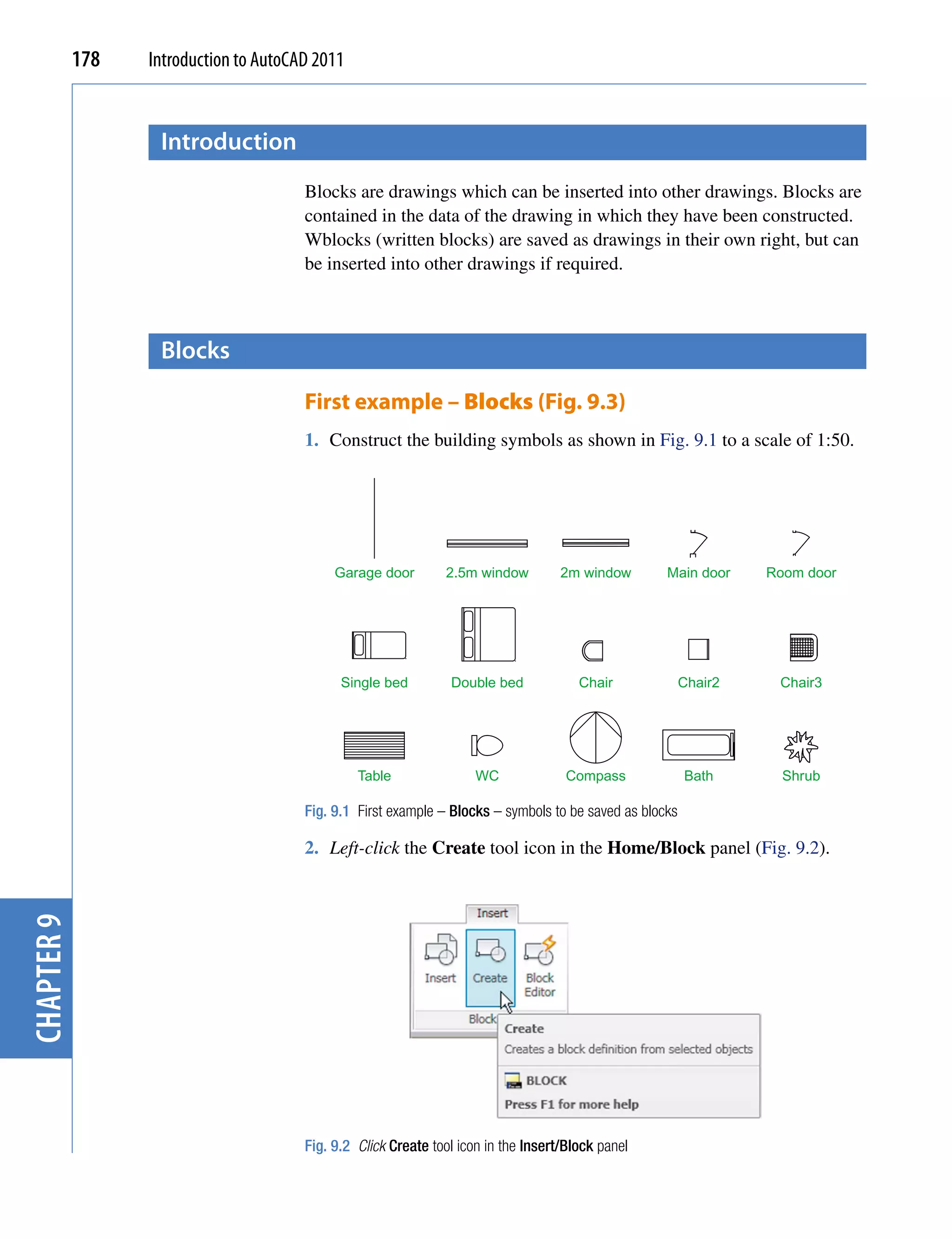
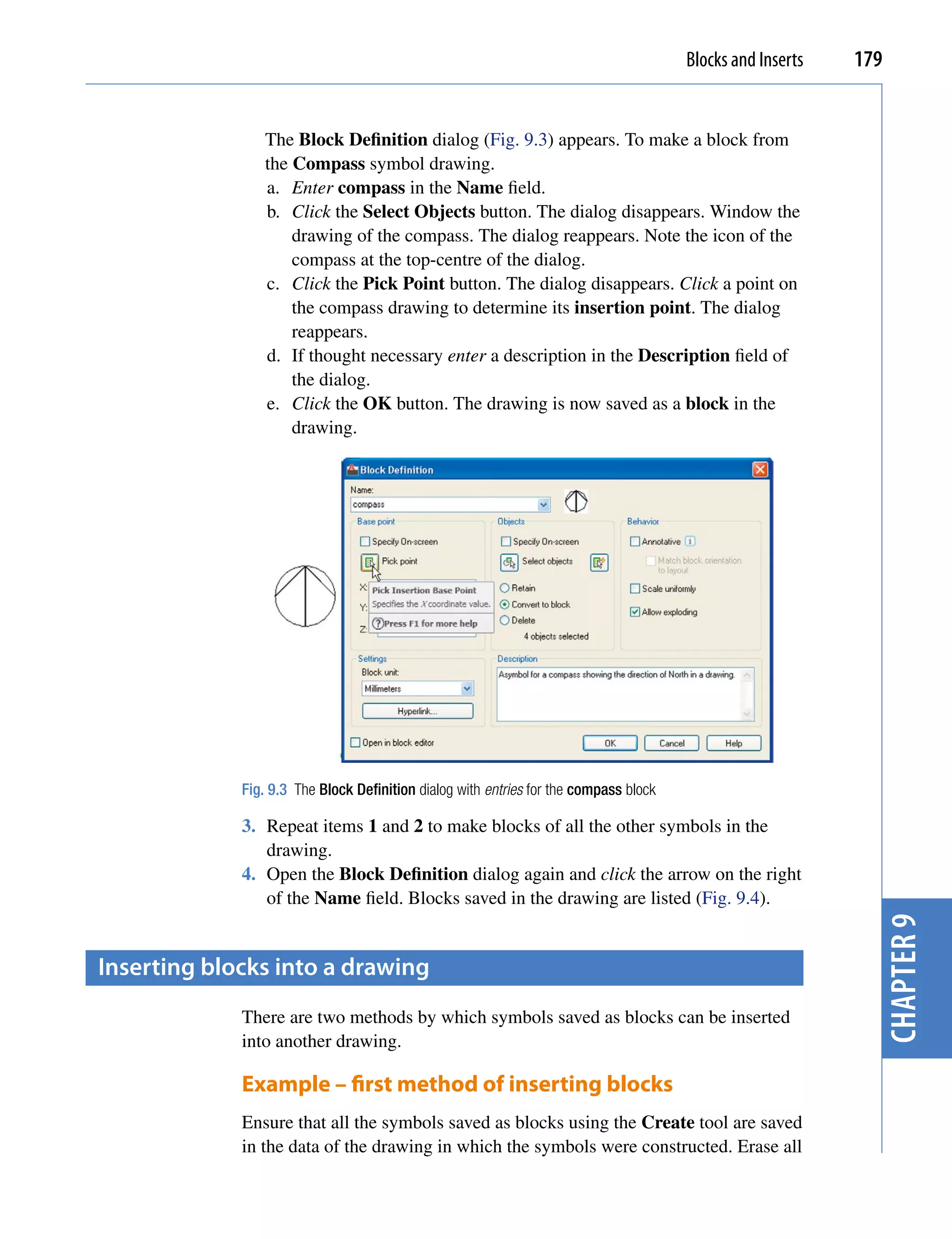
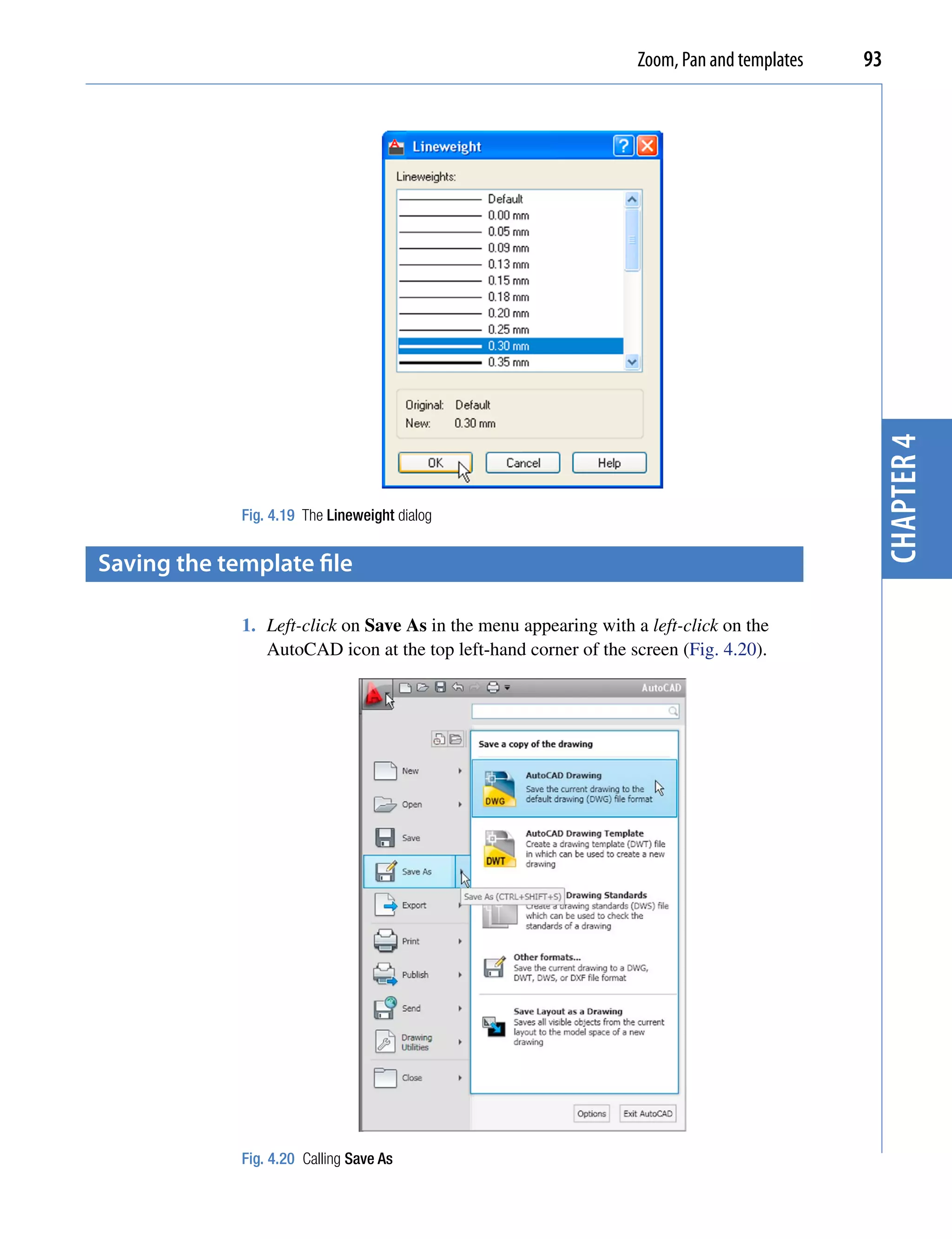
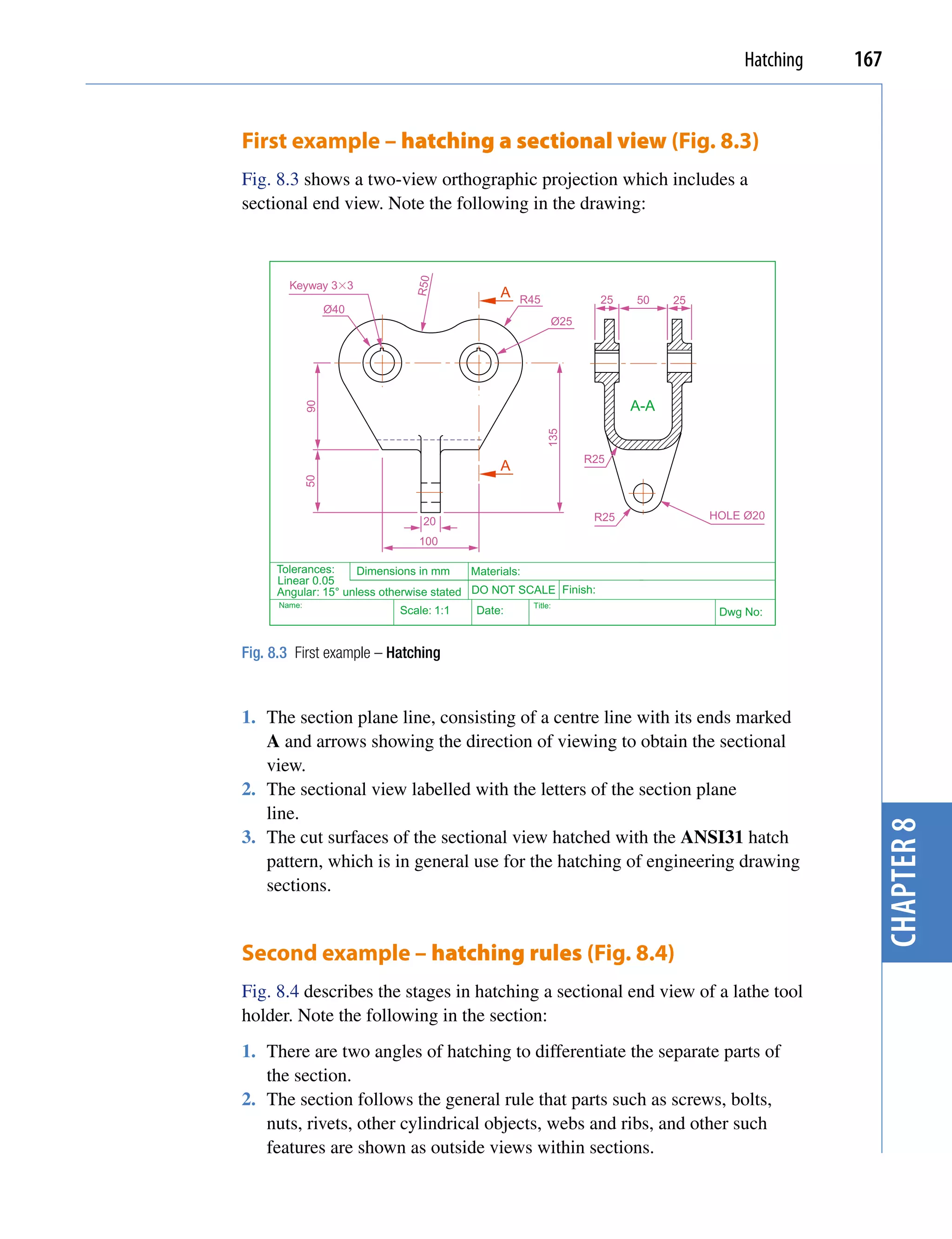
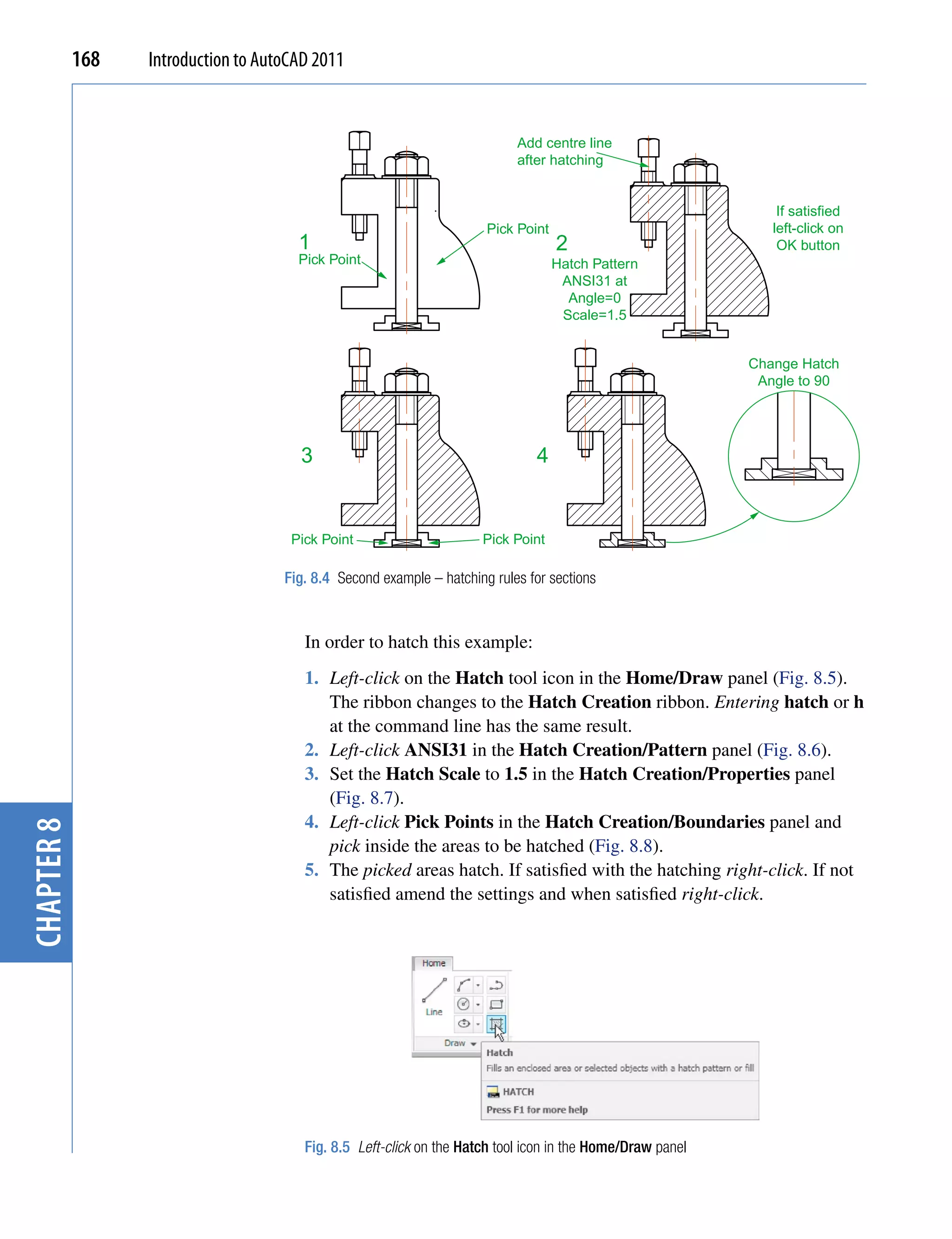
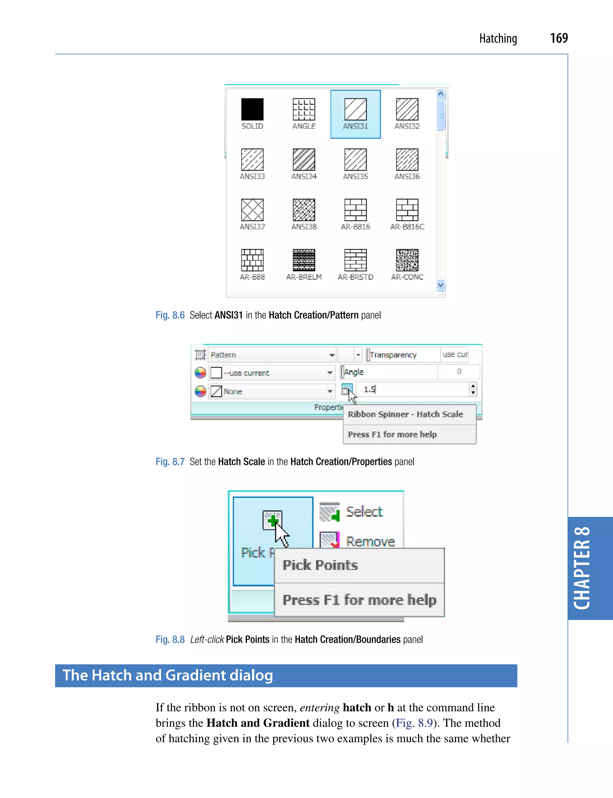
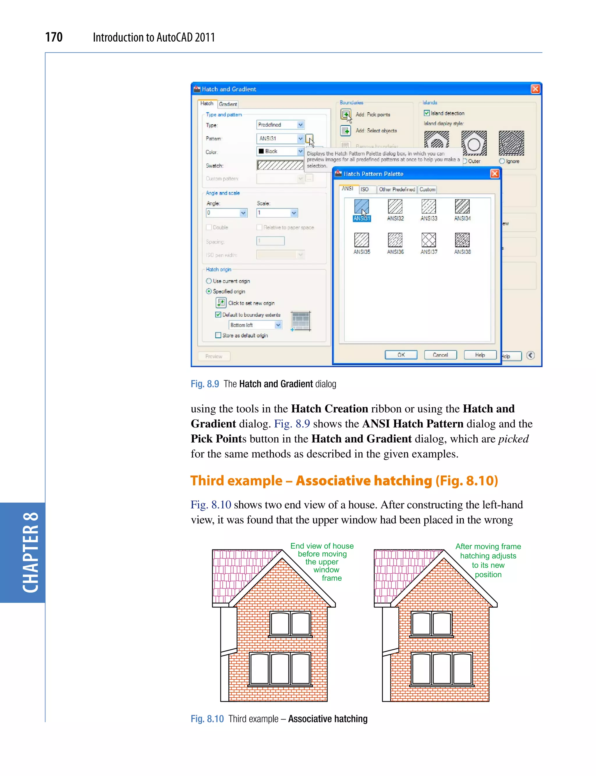
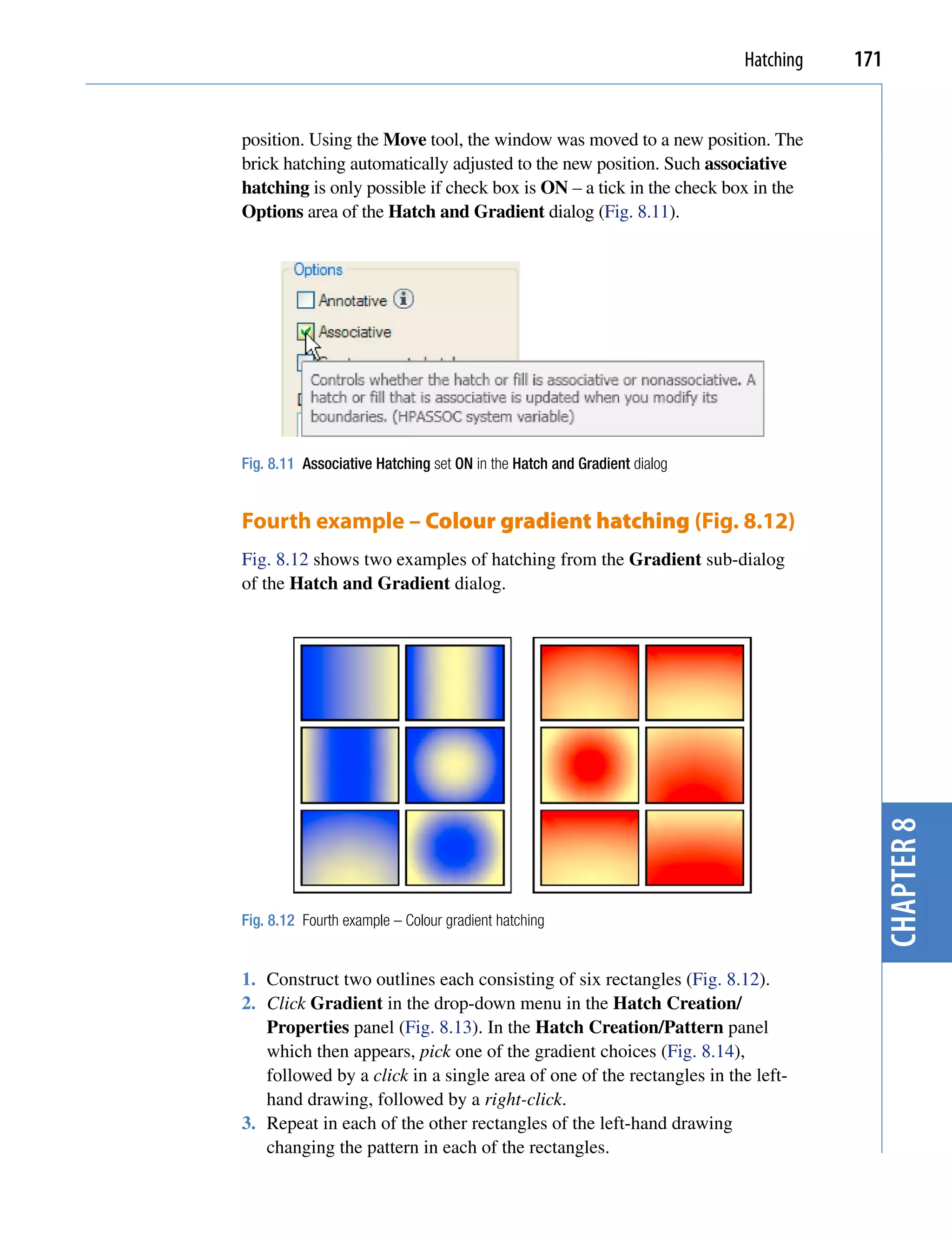
![Blocks and Inserts 181
Fig. 9.6 The Insert tool icon in the Home/Block panel
Fig. 9.7 The Insert dialog with its Name popup list showing all the blocks
required under mouse control. Their angle of position can be amended
at the command line, which shows:
Command:_insert
Specify insertion point or [Basepoint/Scale/
Rotate]: pick
Command:
Selection from these prompts allows scaling or rotating as the block is
inserted.
4. Insert all necessary blocks and add other detail as required to the plan
chapter 9
outline drawing. The result is given in Fig. 9.8.
Example – second method of inserting blocks
1. Save the drawing with all the blocks to a suitable file name. Remember
this drawing includes data of the blocks in its file.
2. Left-click DesignCenter in the View/Palettes panel (Fig. 9.9) or press the
Ctrl2 keys. The DesignCenter palette appears on screen (Fig. 9.10).
3. With the outline plan (Fig. 9.5) on screen the symbols can all be
dragged into position from the DesignCenter.](https://image.slidesharecdn.com/introductiontoautocad2011-100614022653-phpapp02/75/Introduction-to-AutoCad-2011-178-2048.jpg)
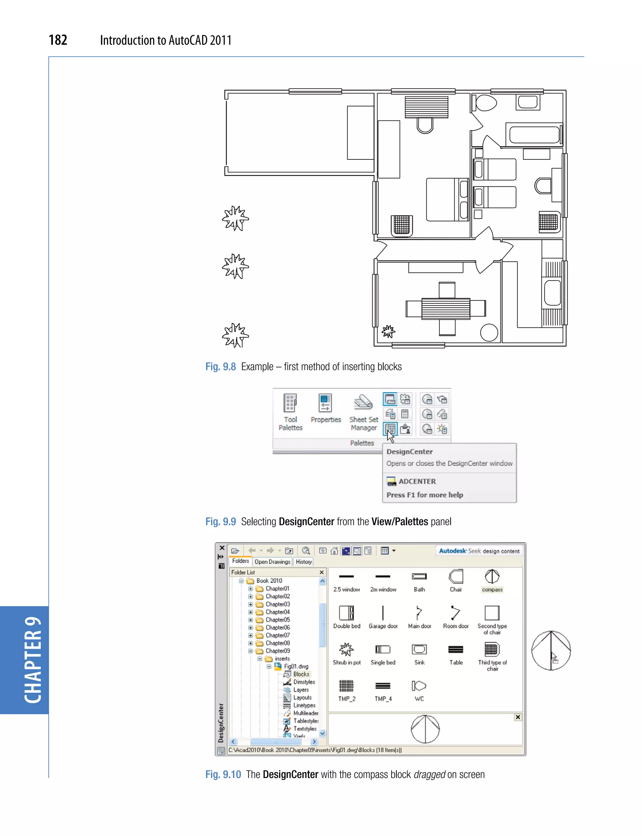
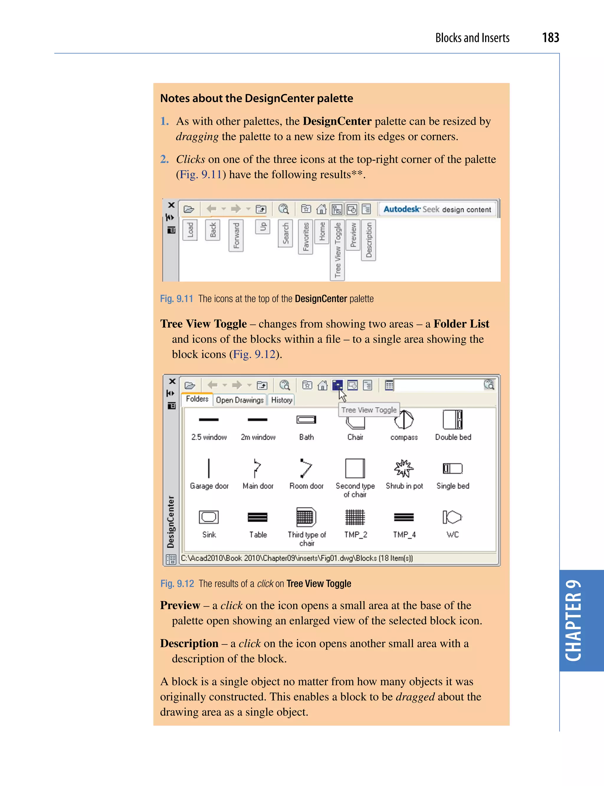
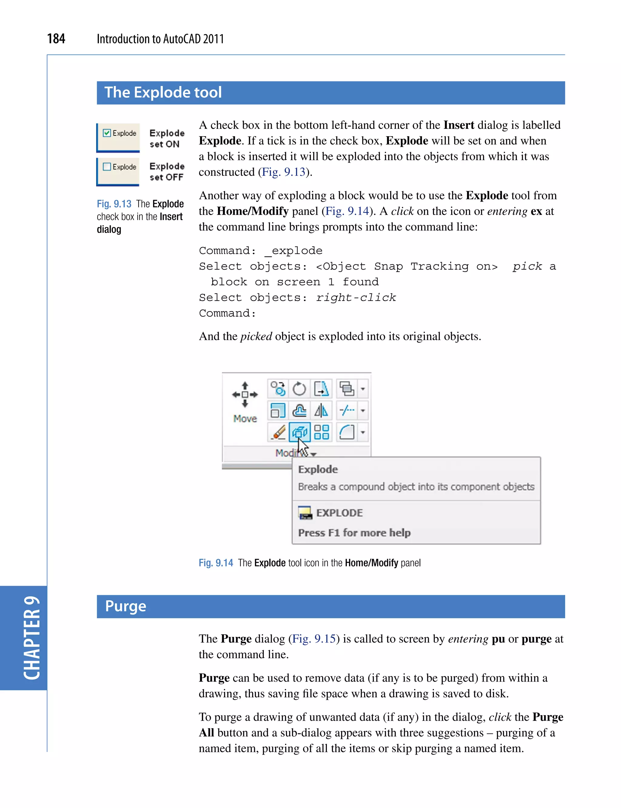
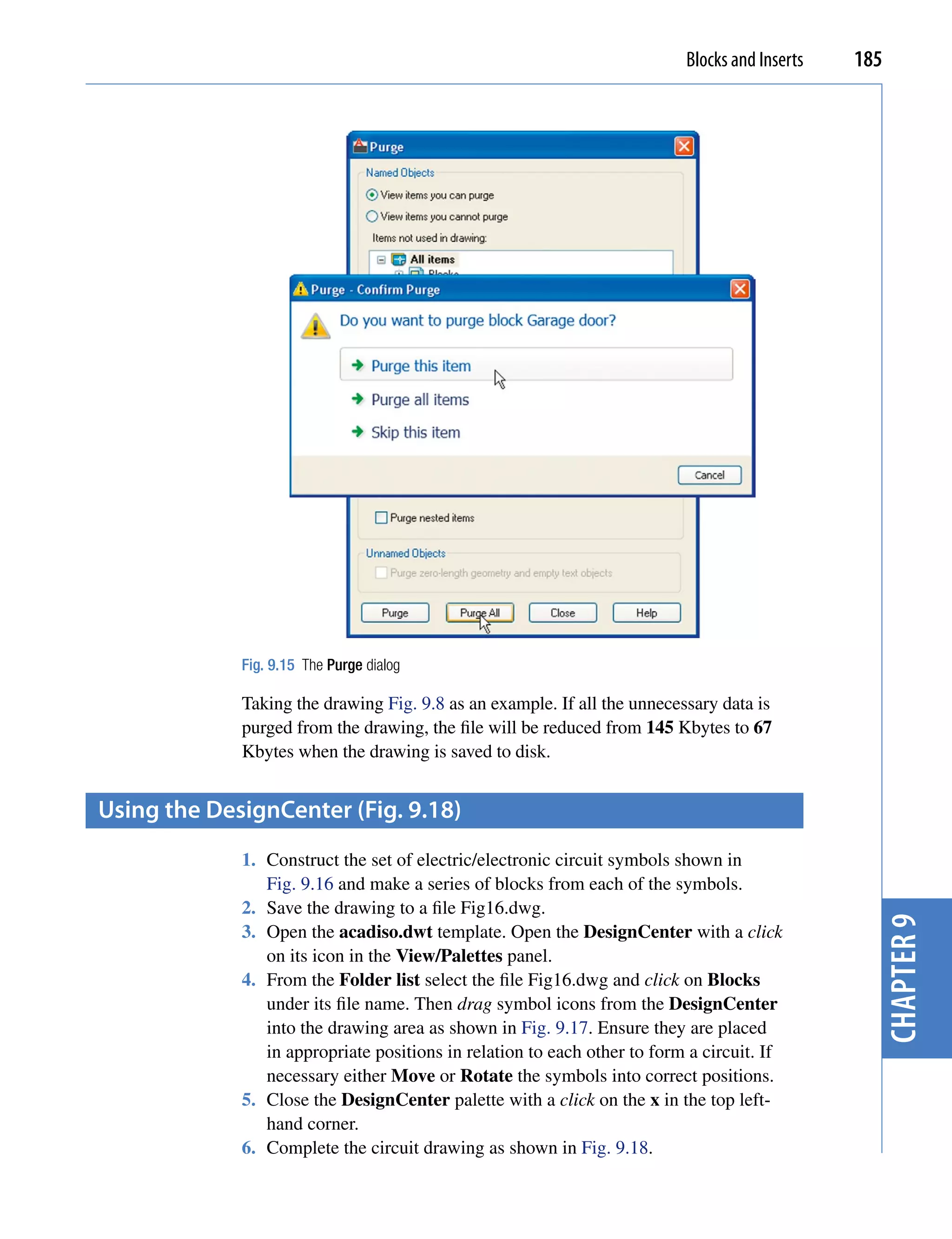
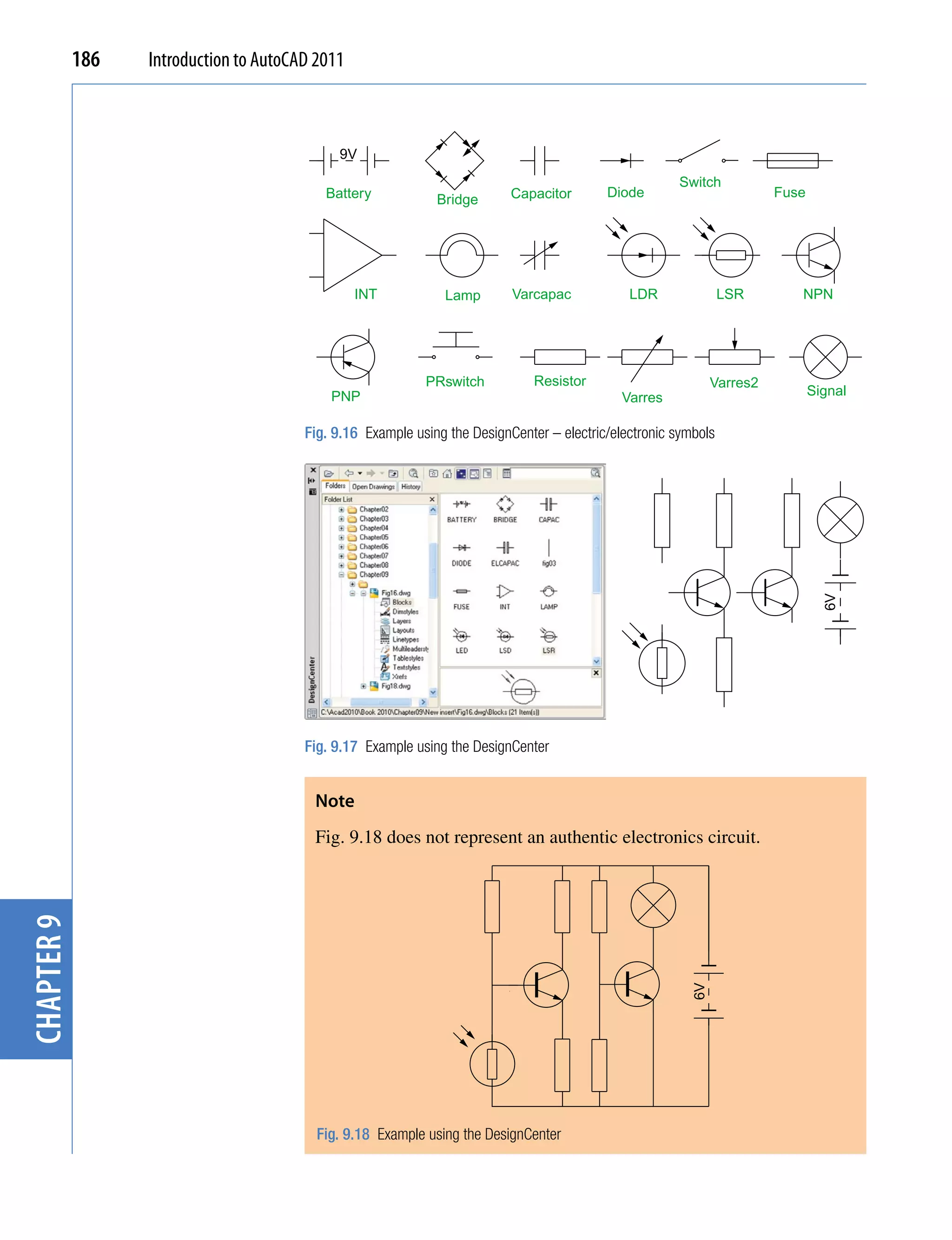
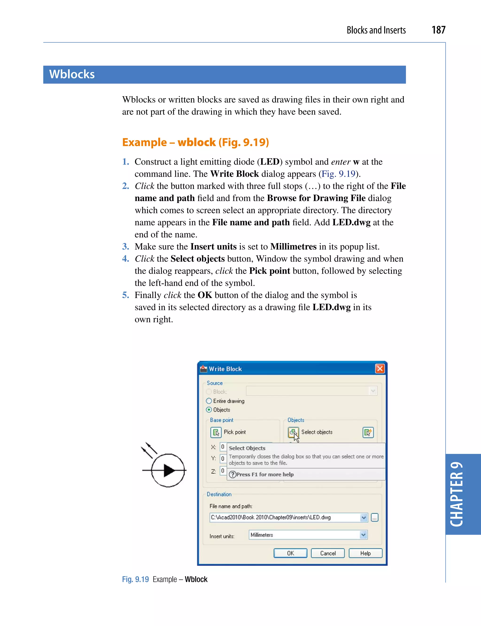
![188 Introduction to AutoCAD 2011
Note on the Designcenter
Drawings can be inserted into the AutoCAD window from the
DesignCenter by dragging the icon representing the drawing into the
window (Fig. 9.20).
Fig. 9.20 An example of a drawing dragged from the DesignCenter
When such a drawing is dragged into the AutoCAD window, the
command line shows a sequence such as:
Command: _-INSERT Enter block name or [?]:
“C:Acad 2011 bookChapter1164
Pheasant DriveFig04.dwg”
Units: Millimeters Conversion: 1.0000
chapter 9
Specify insertion point or [Basepoint/Scale/X/
Y/Z/Rotate]: pick
Enter X scale factor, specify opposite corner,
or [Corner/XYZ] <1>: right-click
Enter Y scale factor <use X scale factor>:
right-click
Specify rotation angle <0>: right-click
Command:](https://image.slidesharecdn.com/introductiontoautocad2011-100614022653-phpapp02/75/Introduction-to-AutoCad-2011-185-2048.jpg)

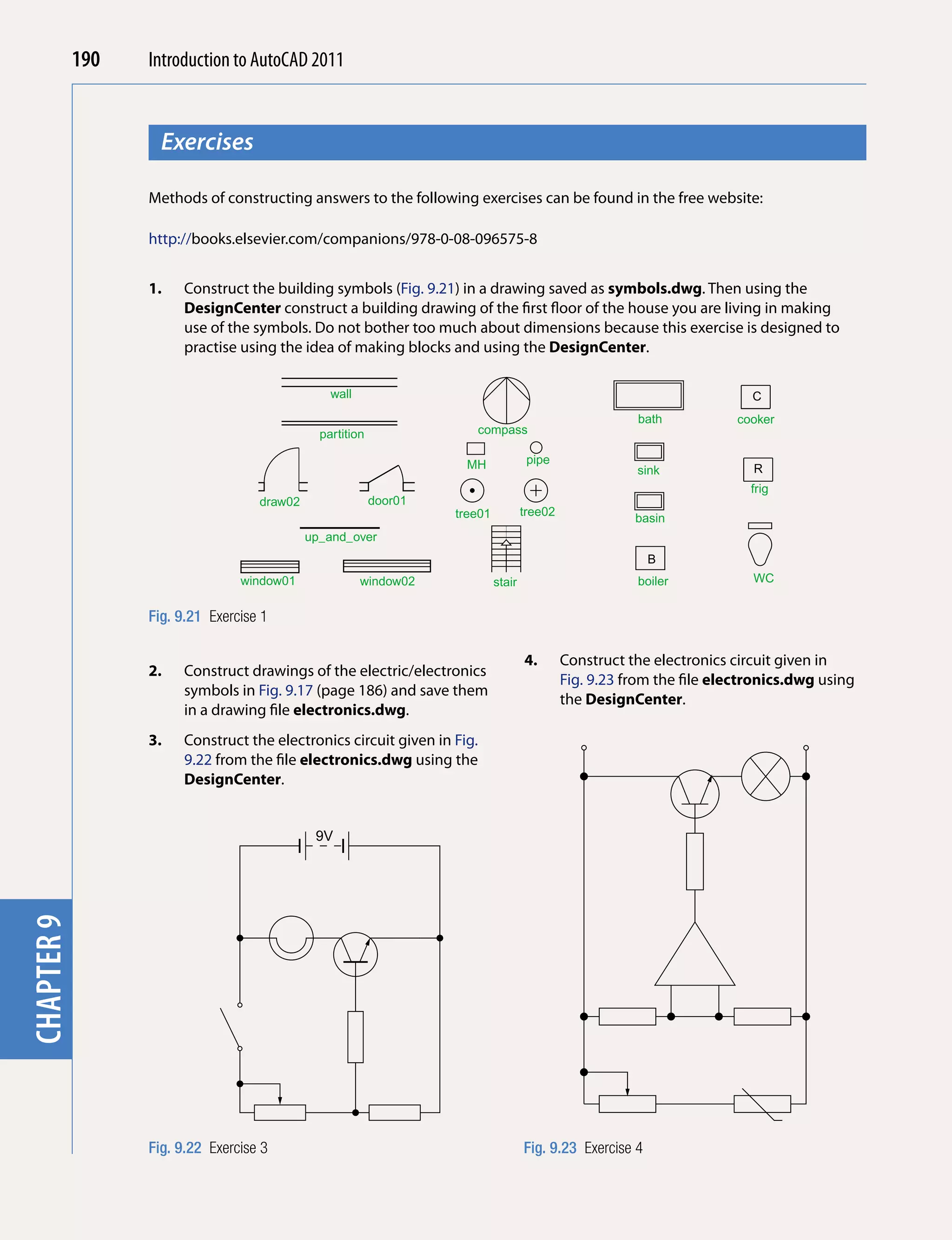
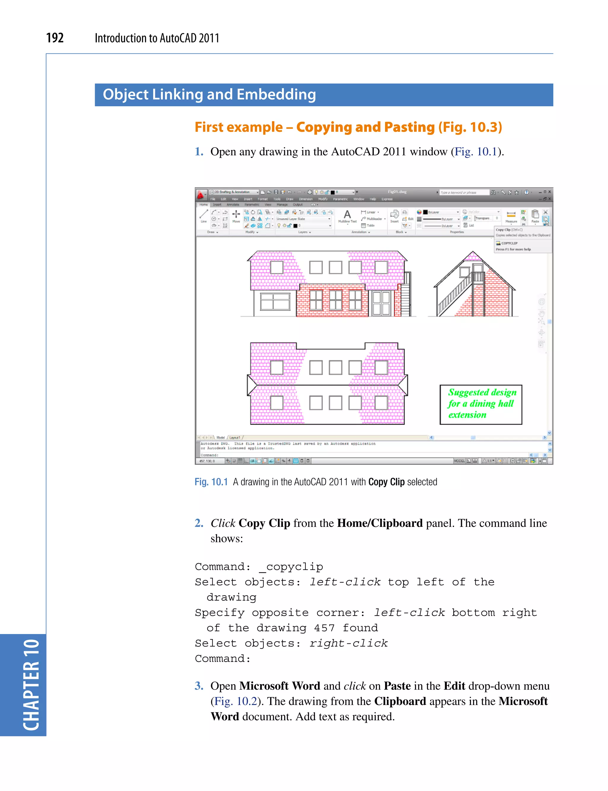
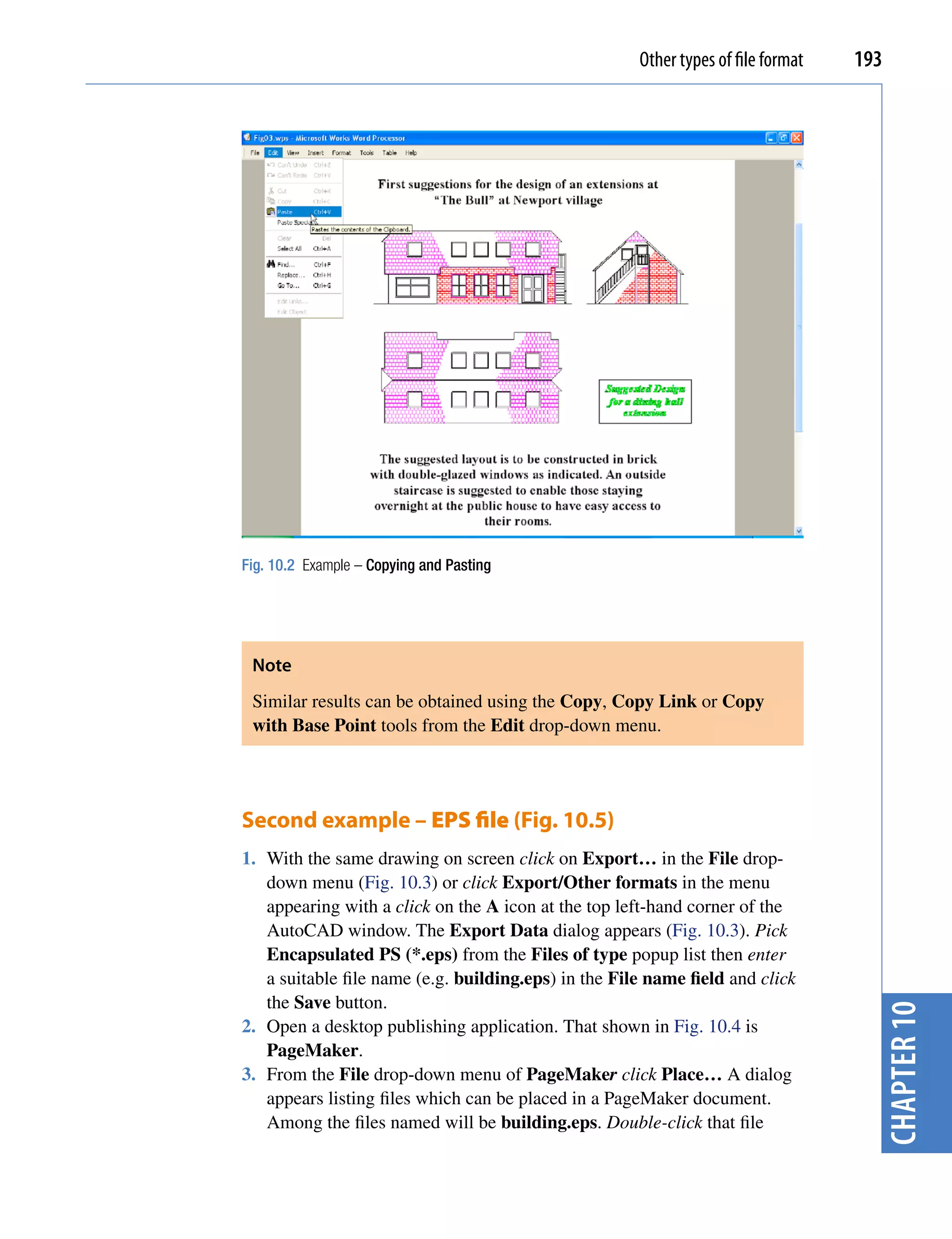
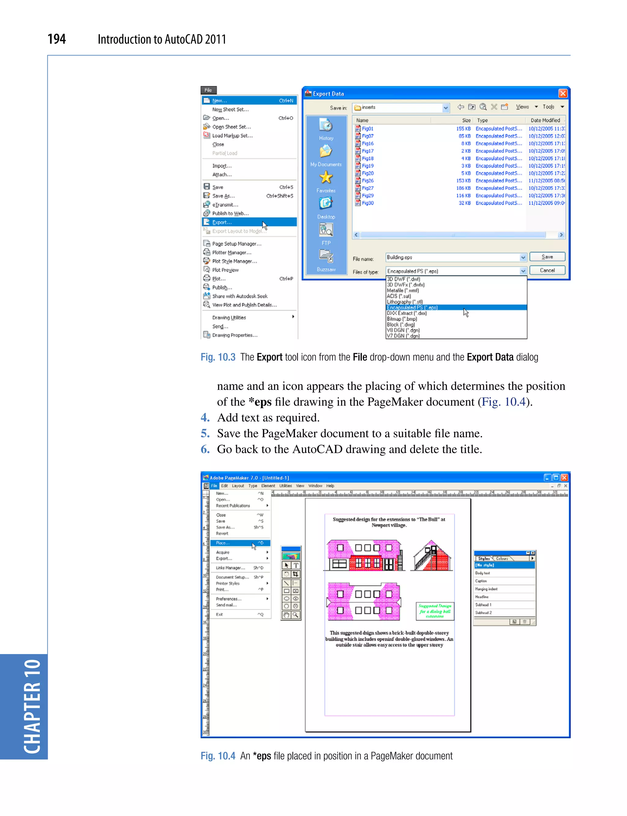
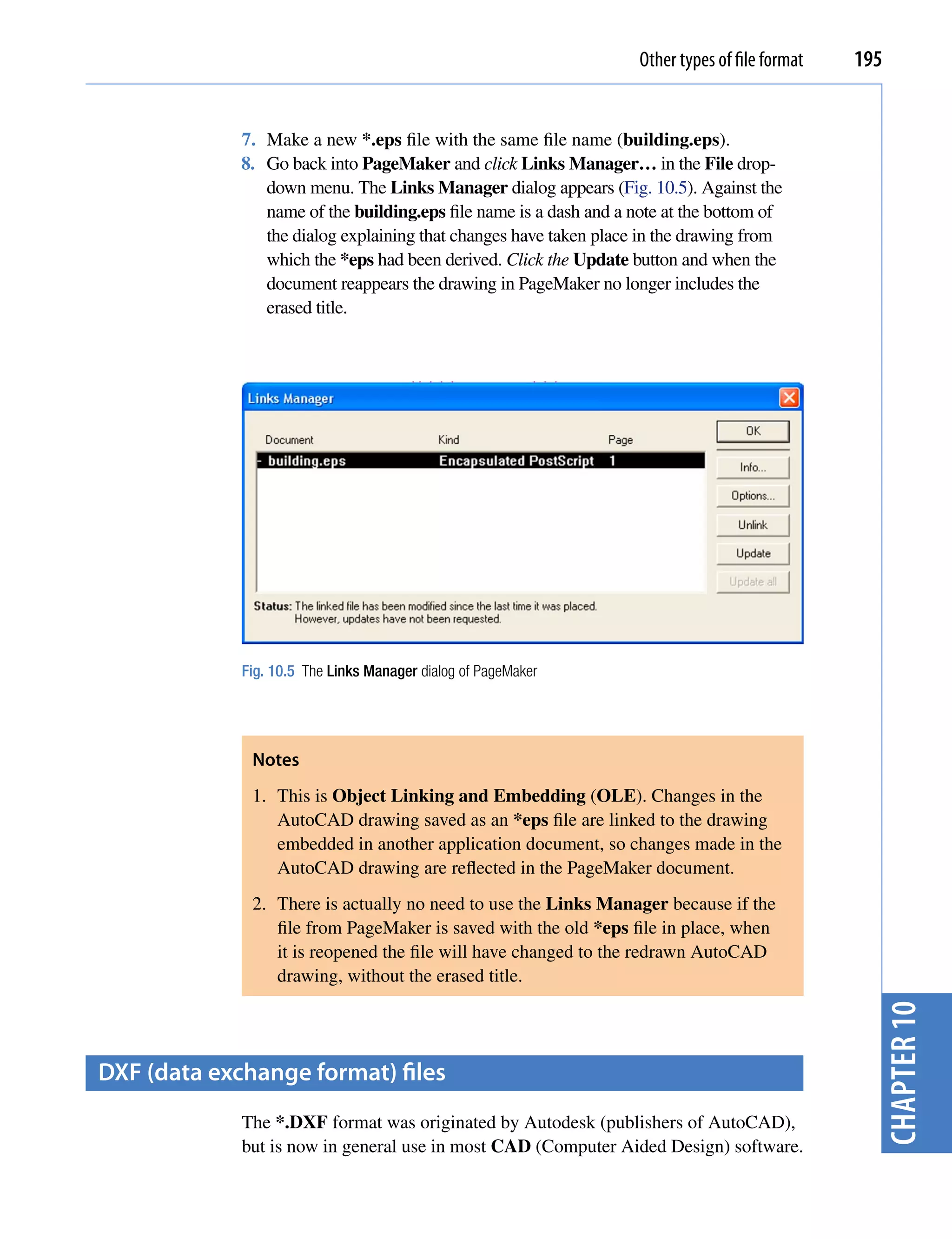
![196 Introduction to AutoCAD 2011
A drawing saved to a *.dxf format file can be opened in most other CAD
software applications. This file format is of great value when drawings are
being exchanged between operators using different CAD applications.
Example – DXF file (Fig. 10.7)
1. Open a drawing in AutoCAD. This example is shown in Fig. 10.6.
Fig. 10.6 Example – DXF file. Drawing to be saved as a dxf file
2. Click on Save As… in the Menu Browser dialog and in the Save
Drawing As dialog which appears, click AutoCAD 2010 DXF [*.dxf]
in the Files of type field popup list.
3. Enter a suitable file name. In this example this is Fig06.dxf. The
extension .dxf is automatically included when the Save button of the
dialog is clicked (Fig. 10.7).
4. The DXF file can now be opened in the majority of CAD applications
and then saved to the drawing file format of the CAD in use.
chapter 10
Note
To open a DXF file in AutoCAD 2011, select Open… from the Menu
Browser dialog and in the Select File dialog select DXF [*.dxf] from
the popup list from the Files of type field.](https://image.slidesharecdn.com/introductiontoautocad2011-100614022653-phpapp02/75/Introduction-to-AutoCad-2011-193-2048.jpg)
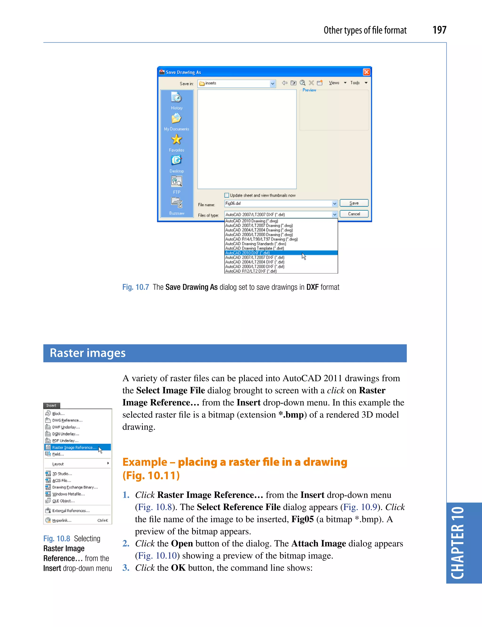
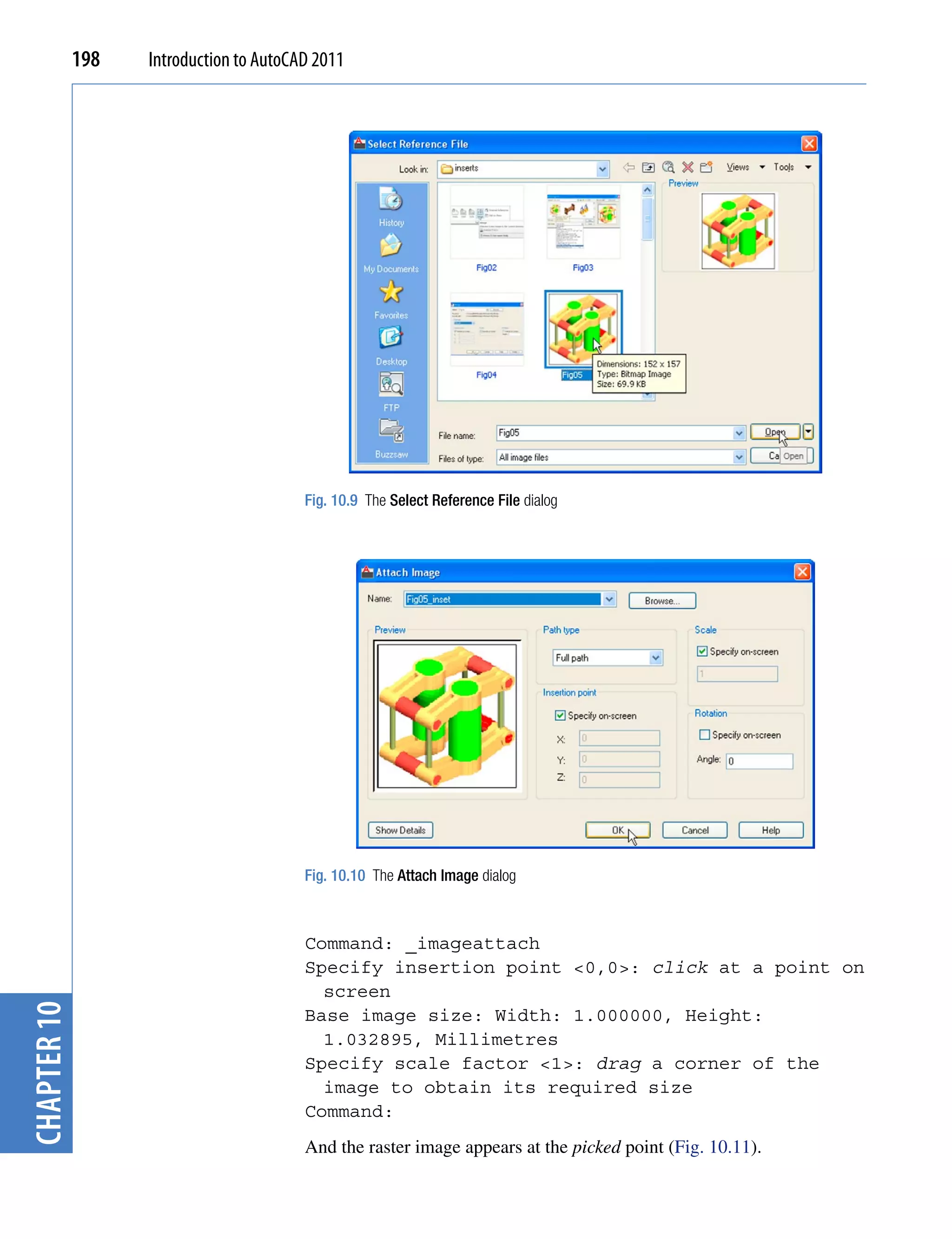
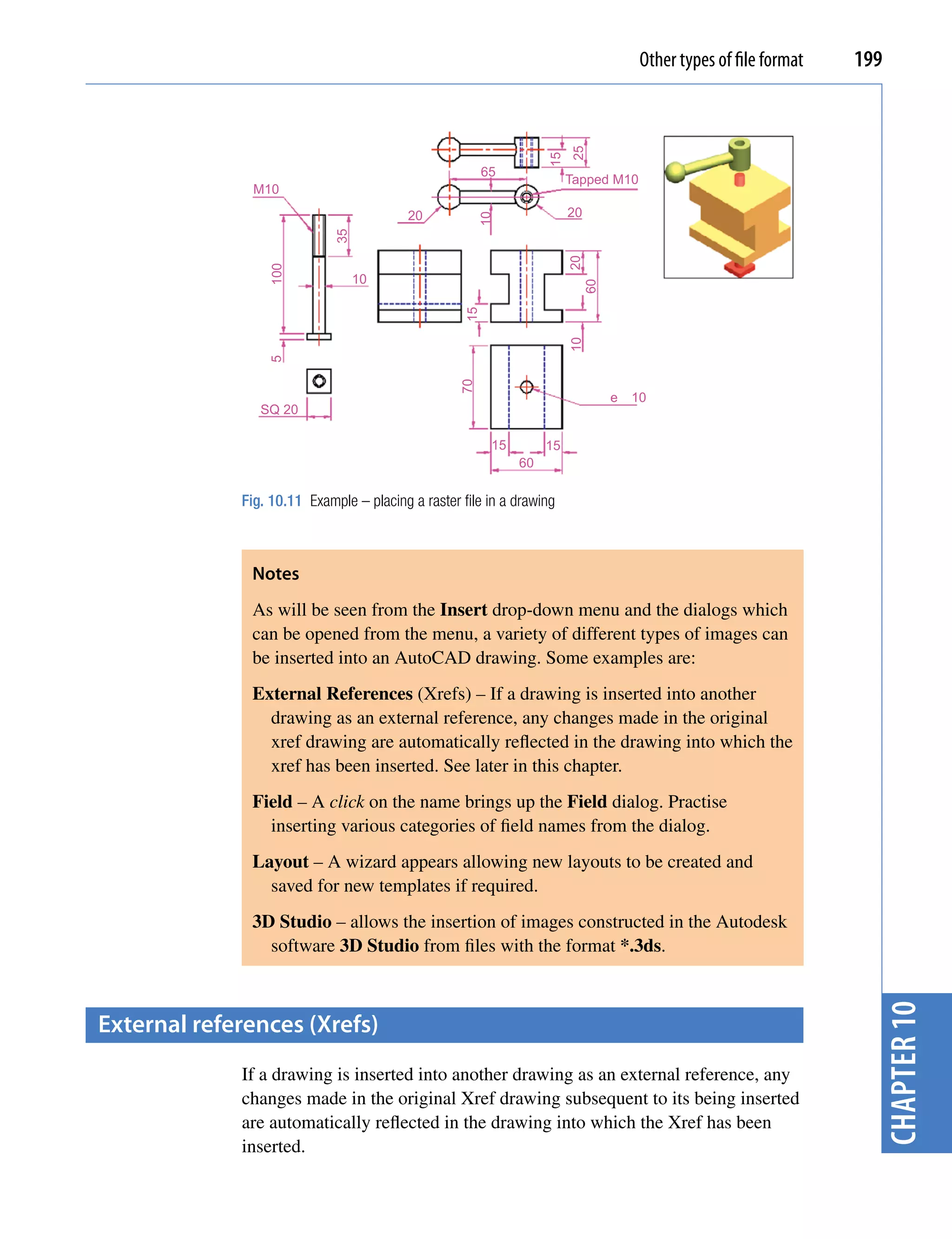
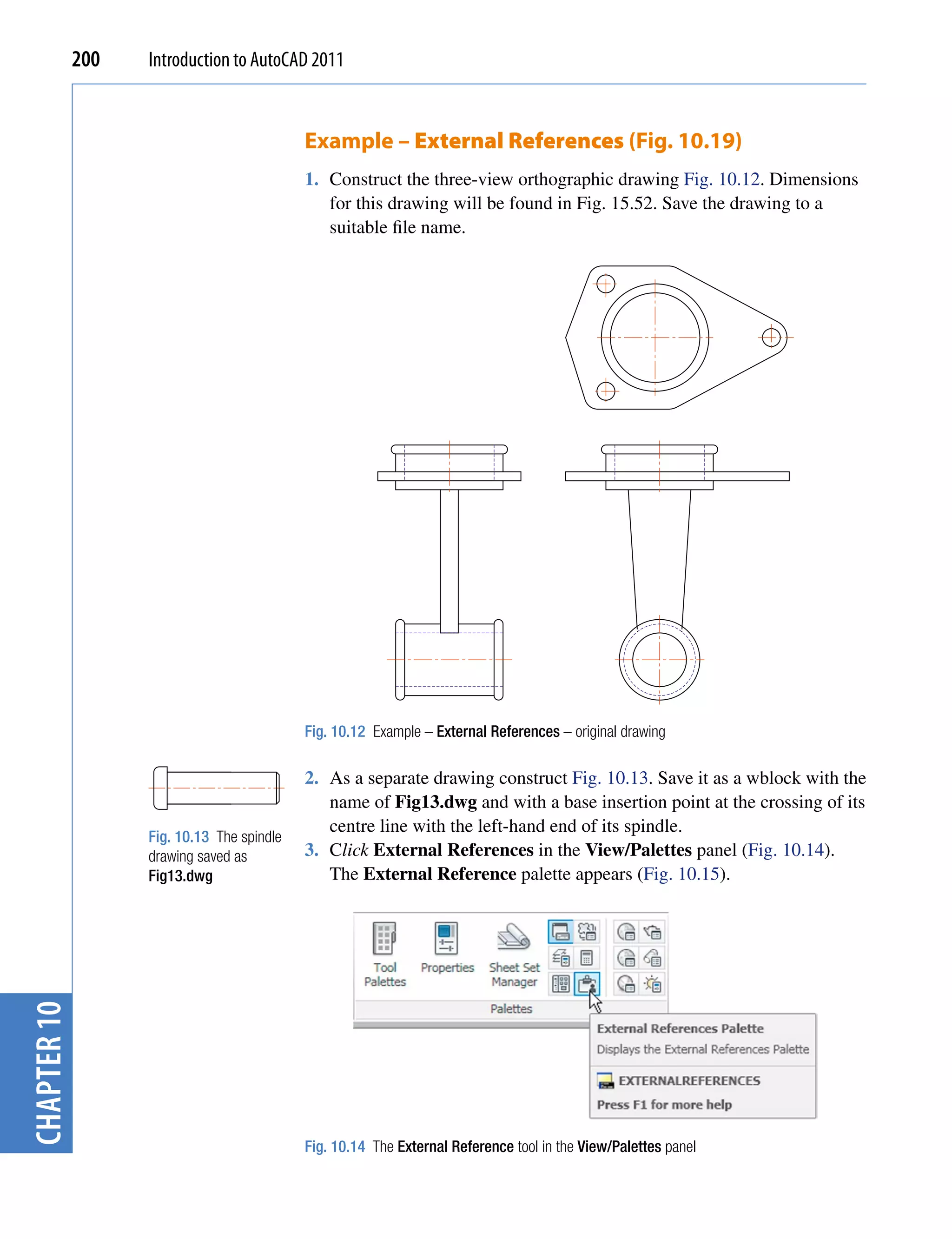
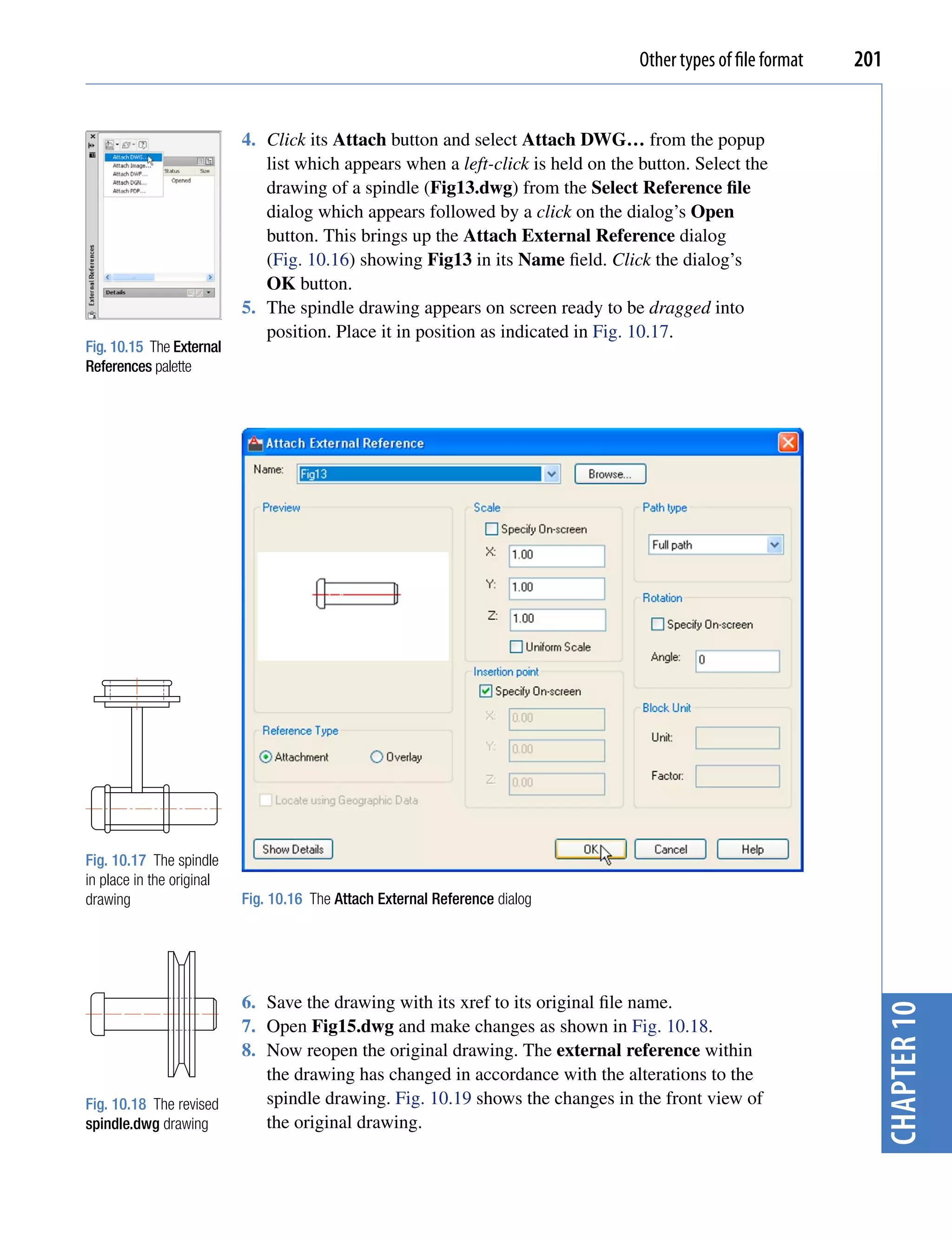
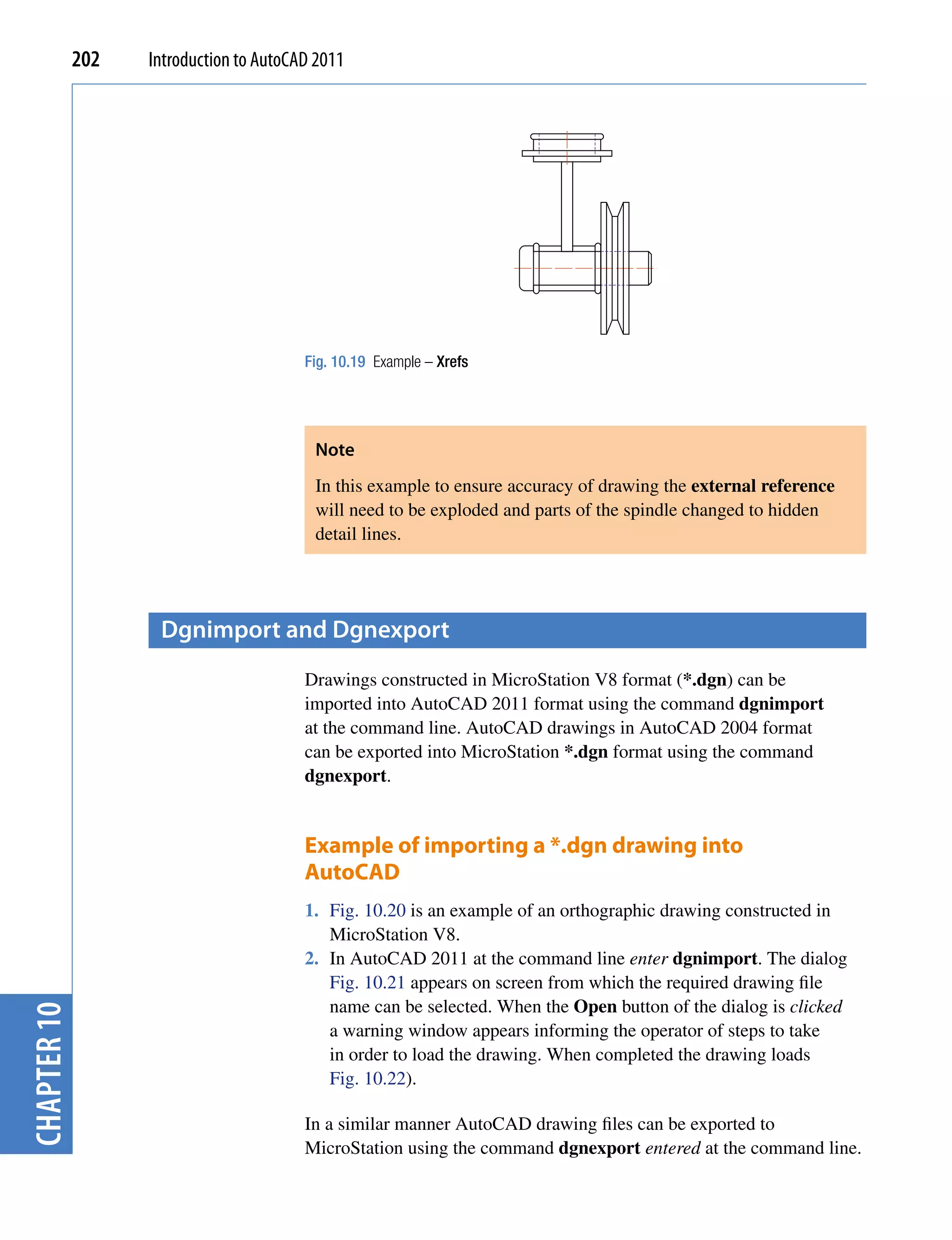
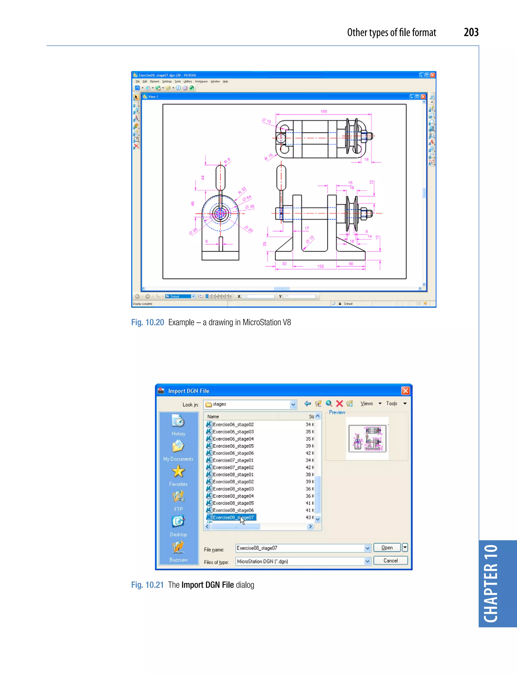
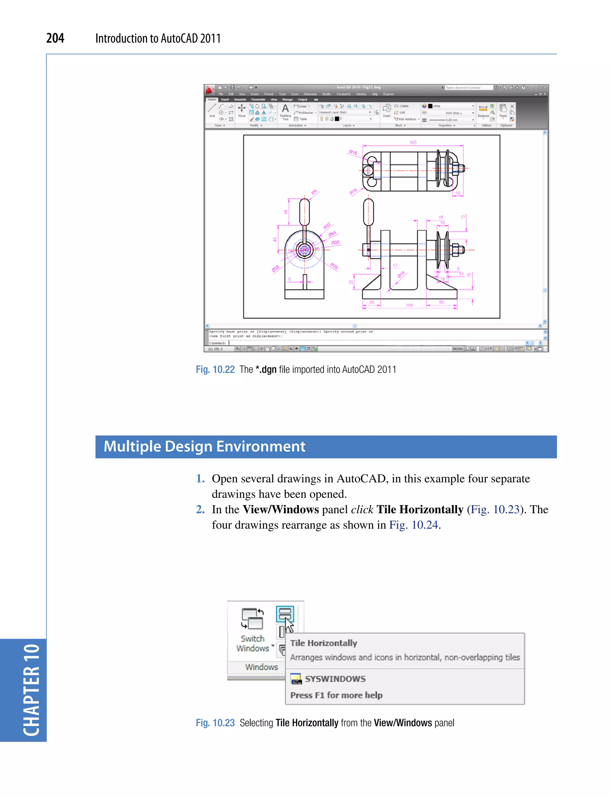
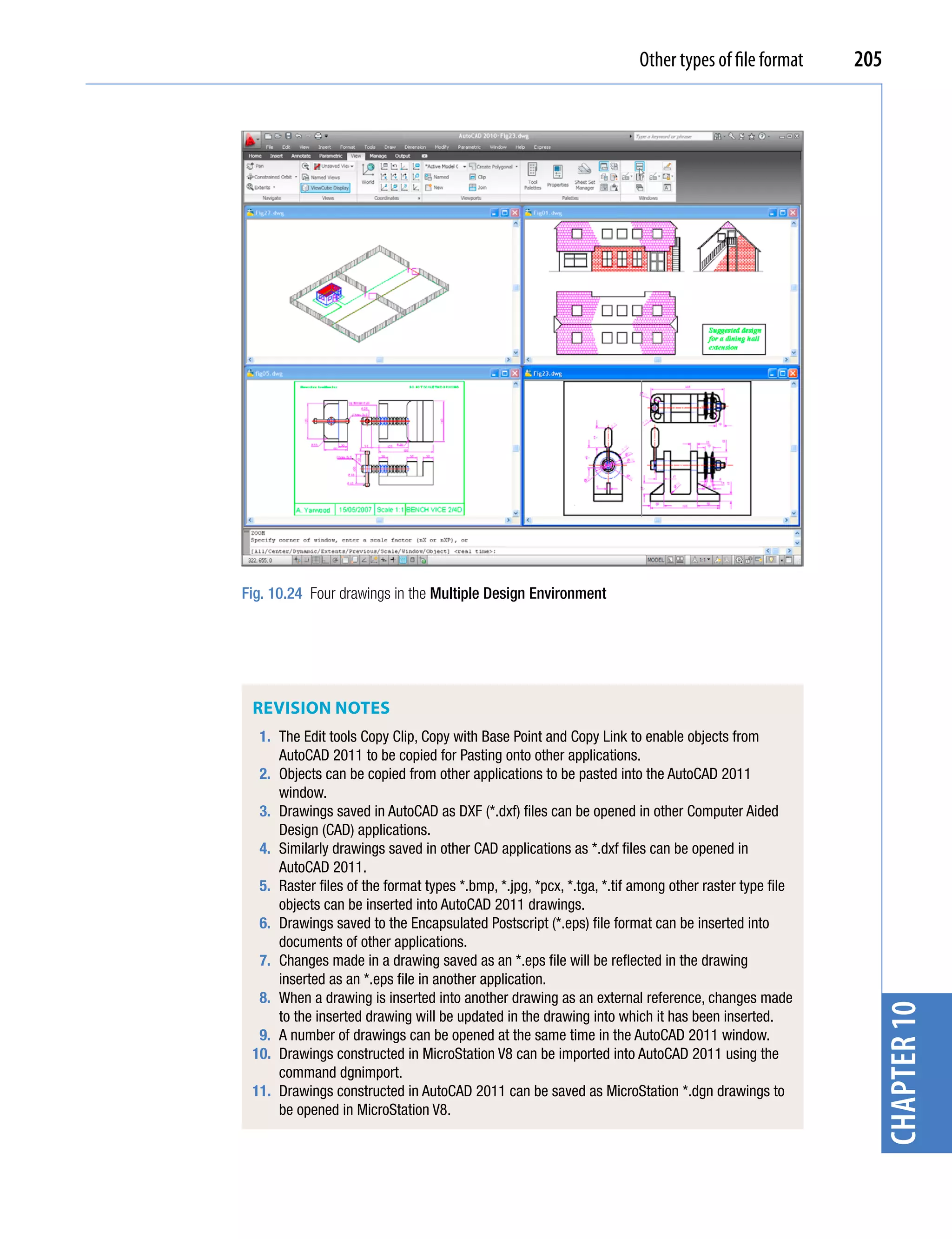
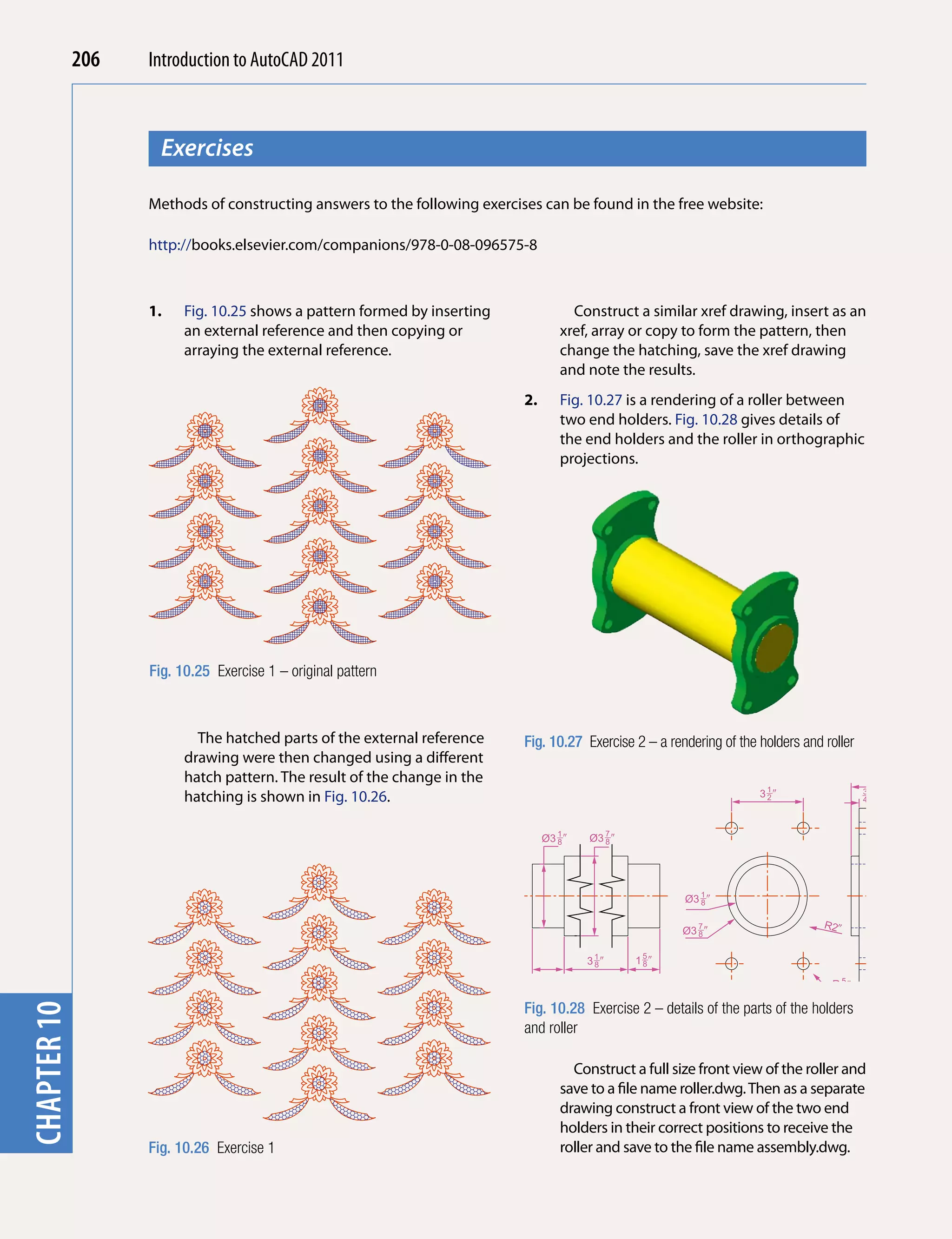
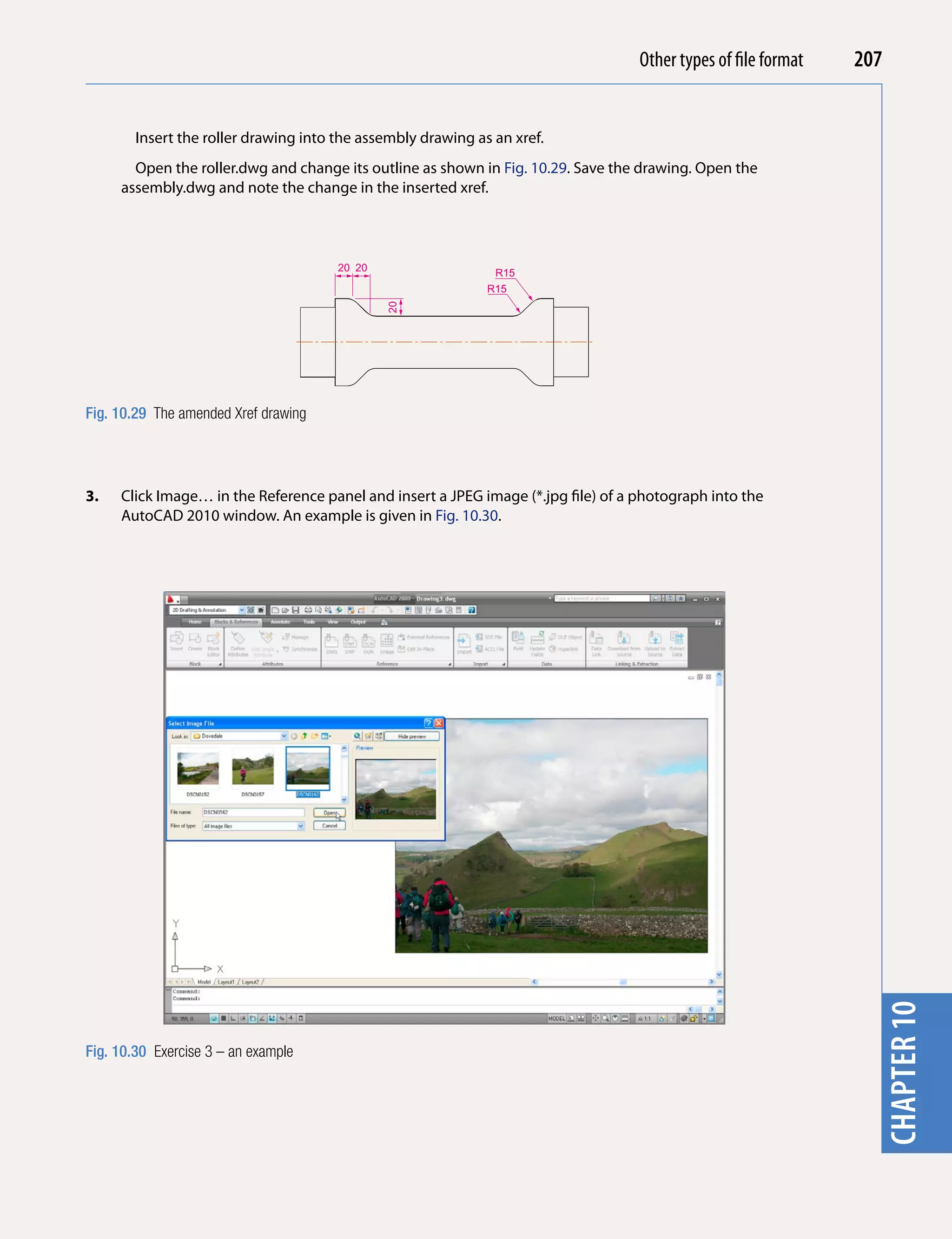
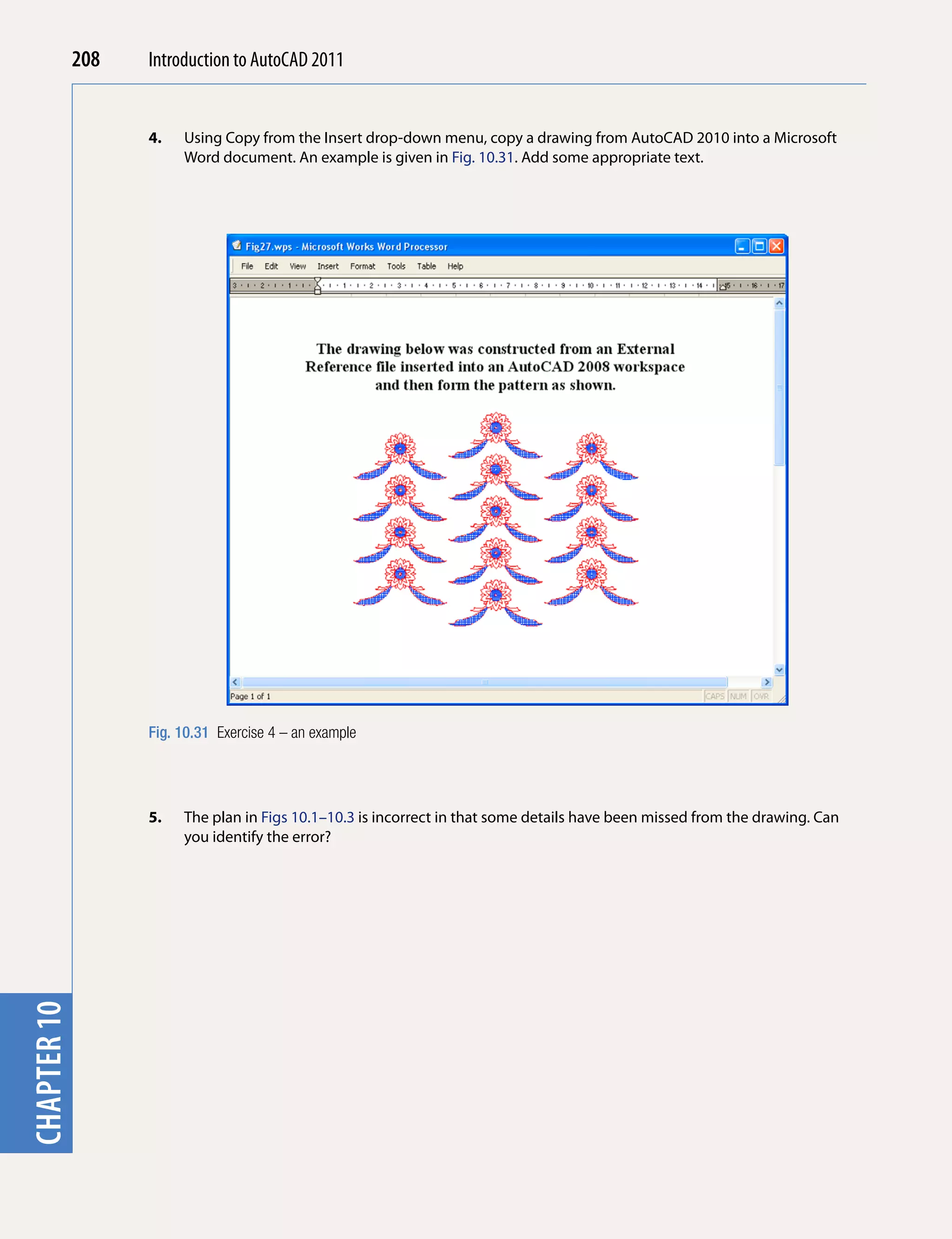

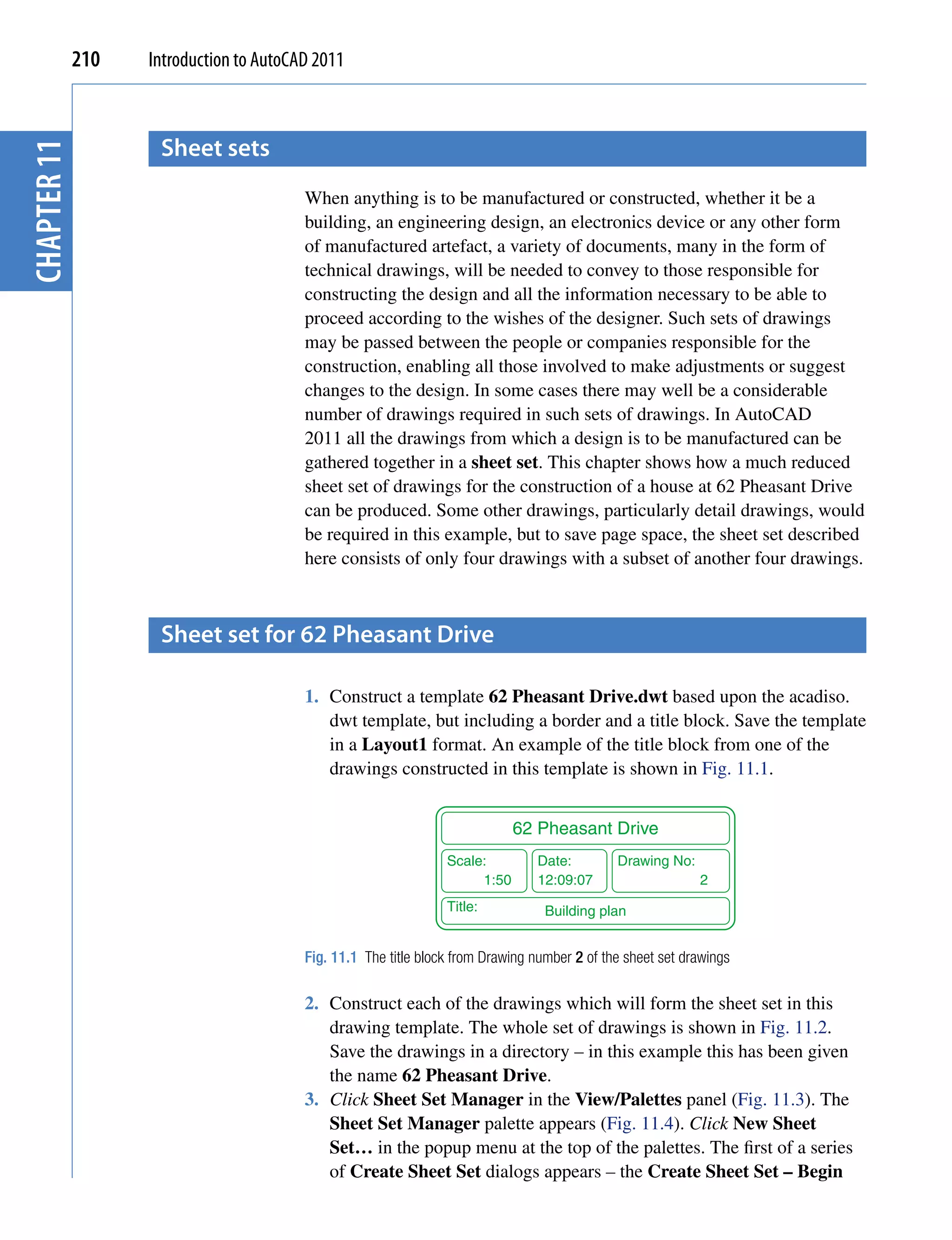
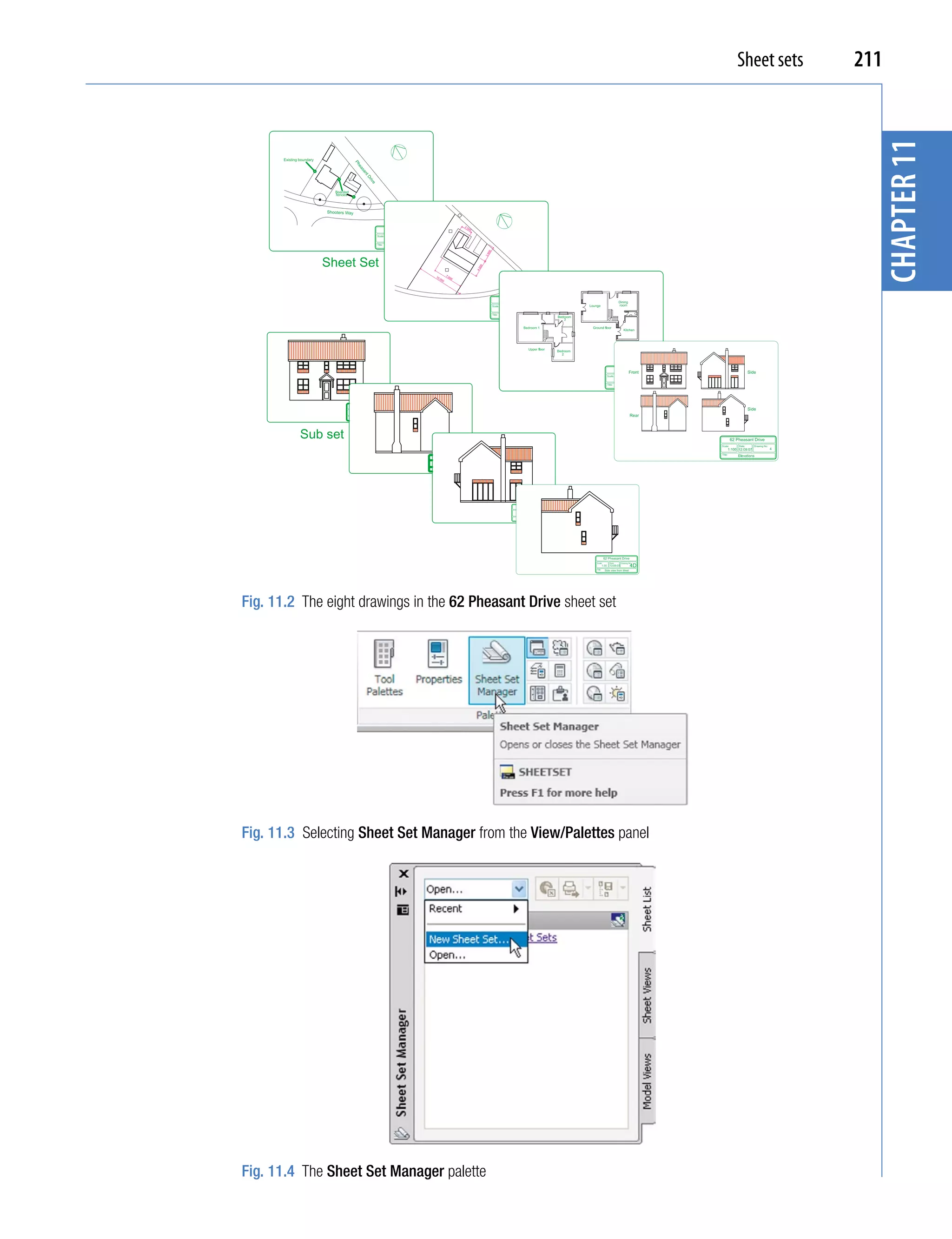
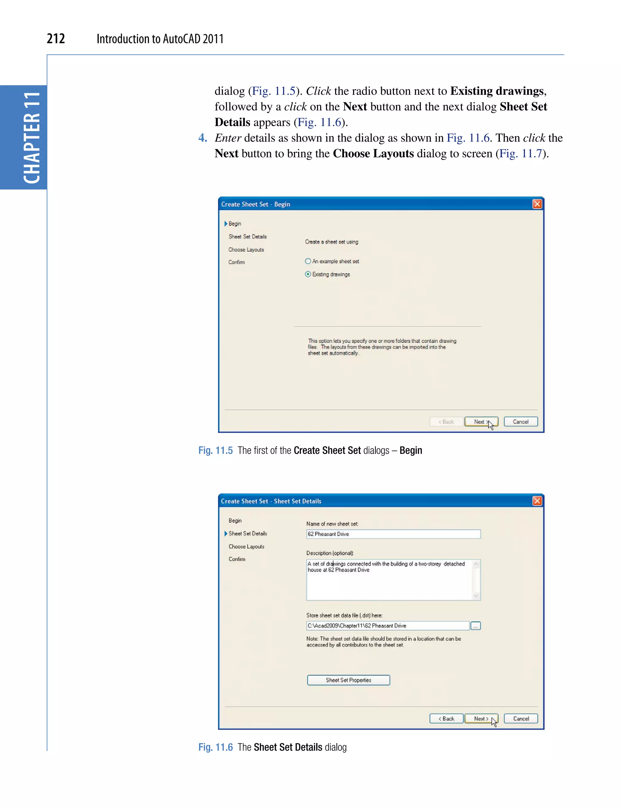
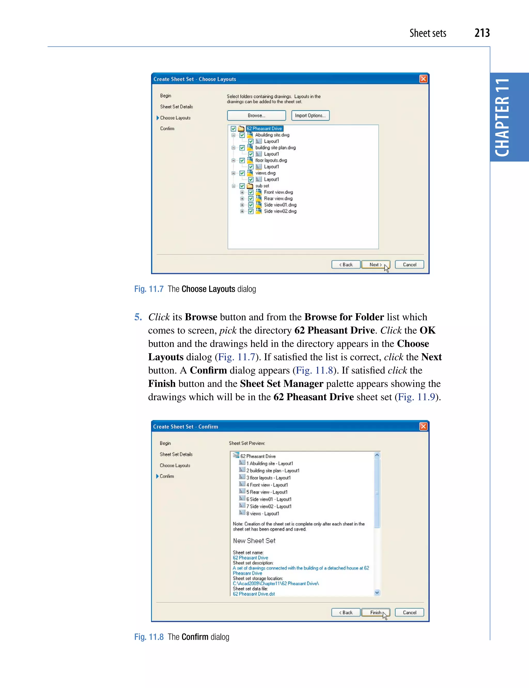
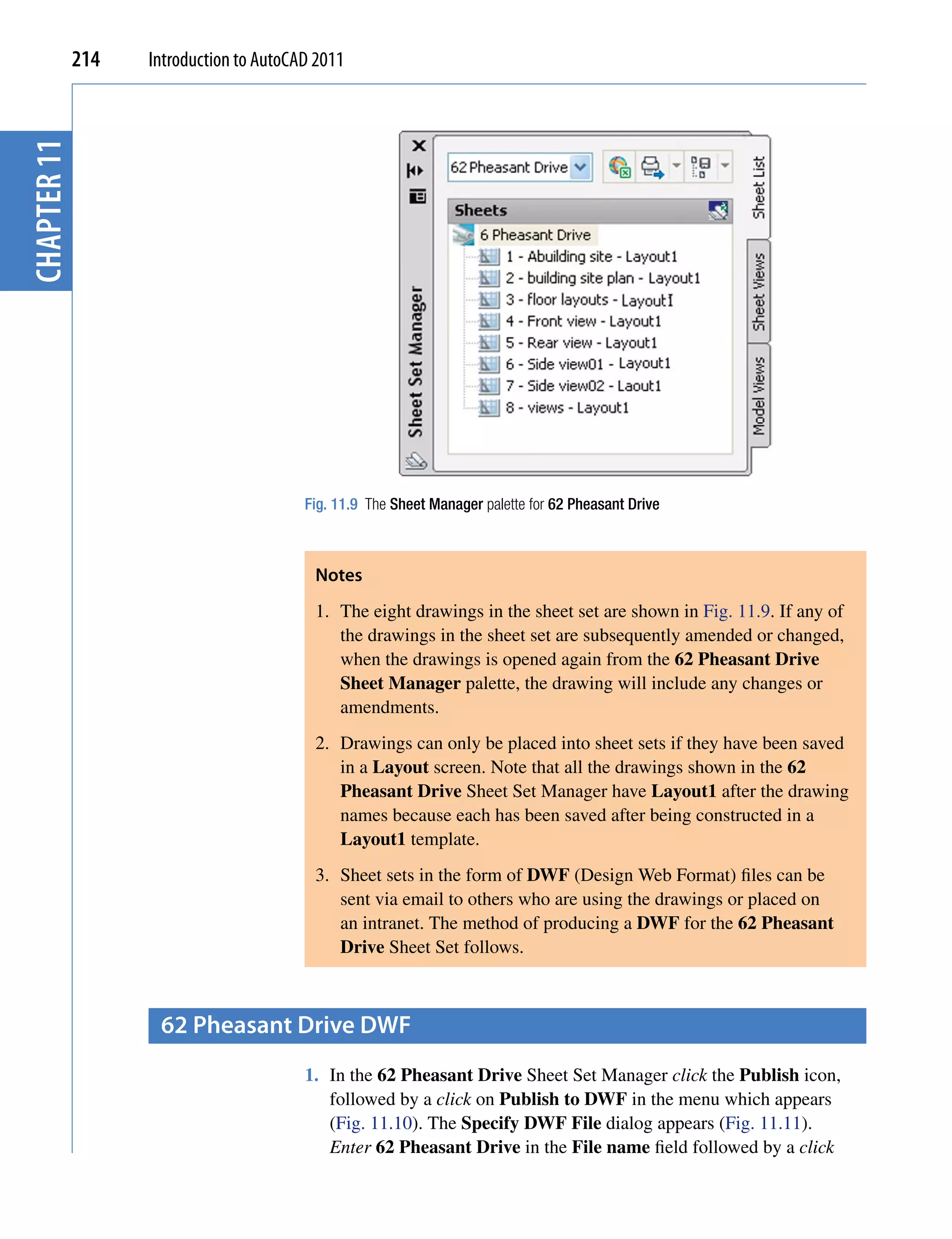
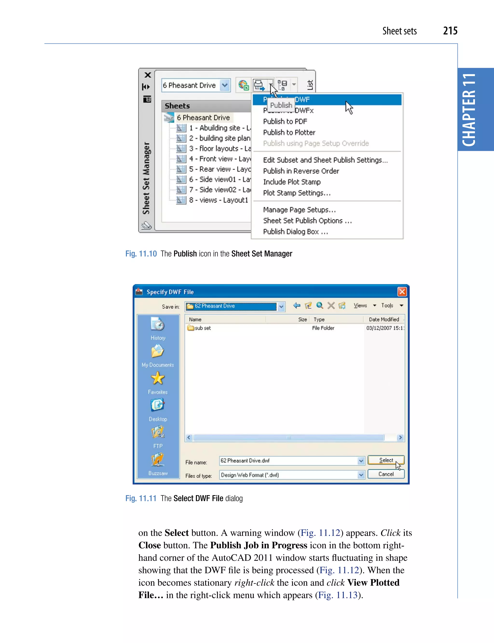
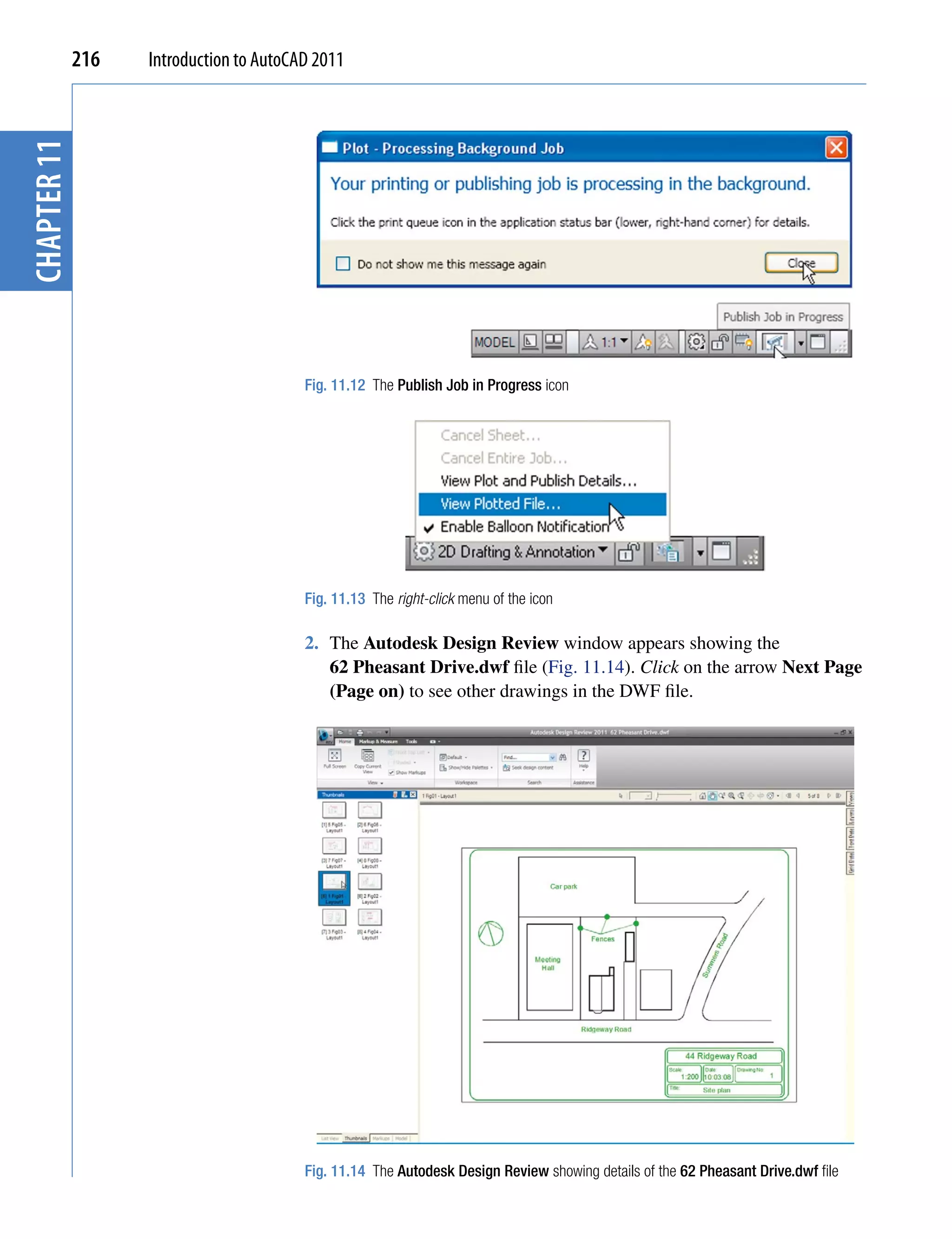

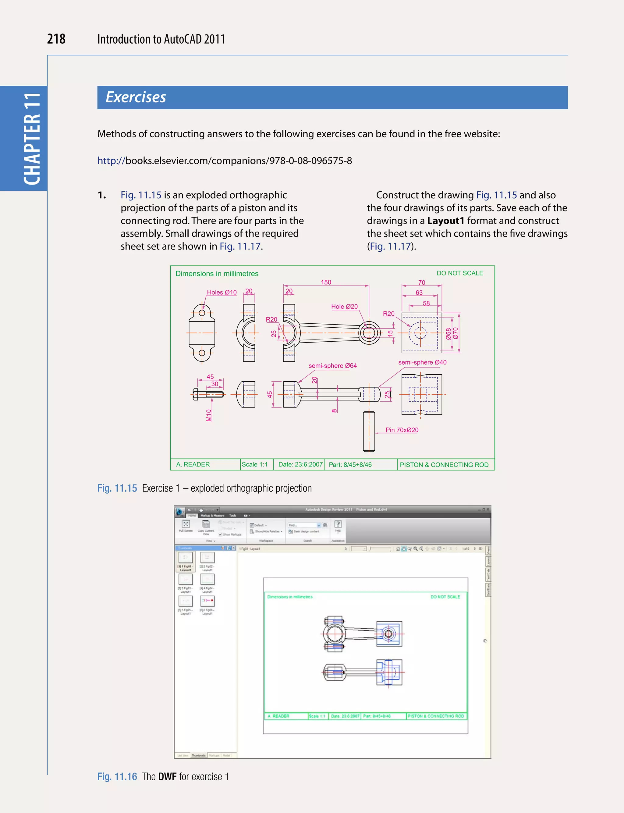
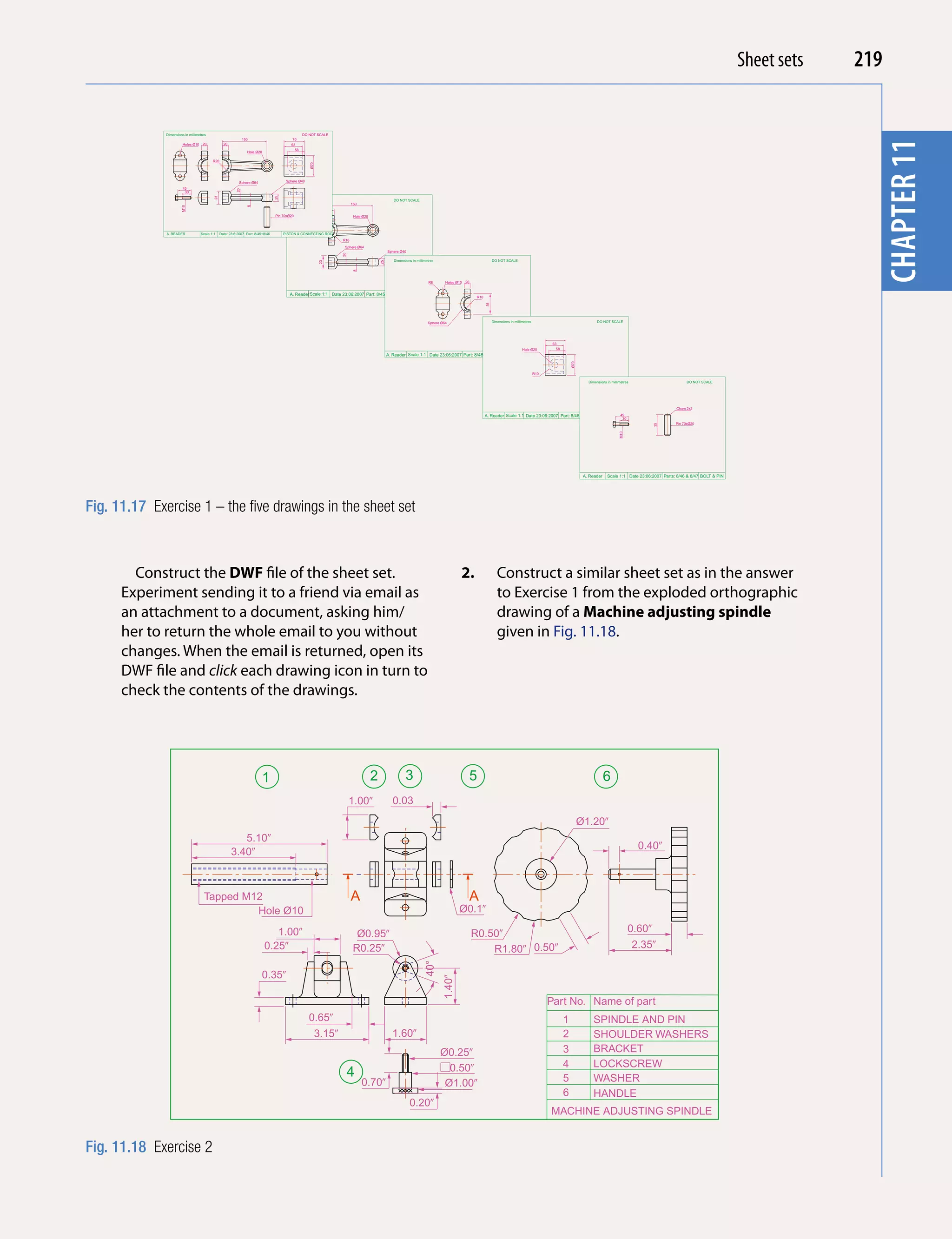
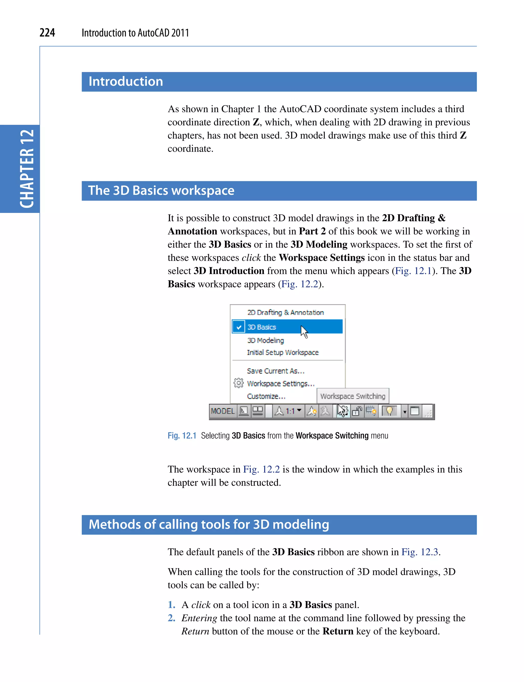
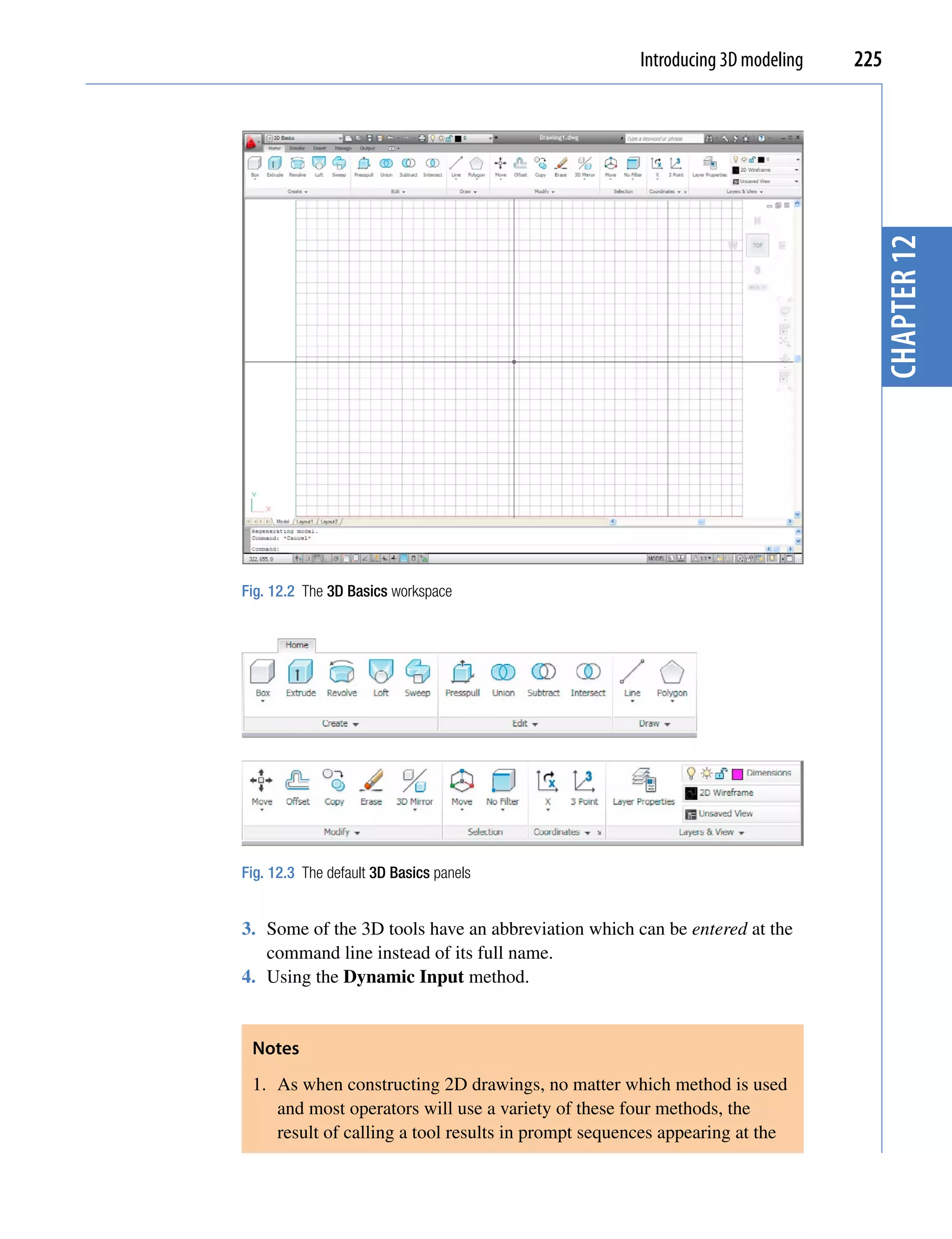
![226 Introduction to AutoCAD 2011
command prompt (or if using Dynamic Input on screen) as in the
following example:
Command: enter box right-click
Specify first corner or [Center]: enter 90,120
chapter 12
right-click
Specify other corner or [Cube/Length]: enter
150,200
Specify height or [2Point]: enter 50
Command:
Or, if the tool is called from its tool icon, or from a drop-down menu:
Command:_box
Specify first corner or [Center]: enter 90,120
right-click
Specify other corner or [Cube/Length]: enter
150,200
Specify height or [2Point]: enter 50
Command:
2. In the following pages, if the tool’s sequences are to be repeated,
they may be replaced by an abbreviated form such as:
Command: box
[prompts]: 90,120
[prompts]: 150,200
3. The examples shown in this chapter will be based on layers set as
follows:
a. Click the Layer Properties icon in the Home/Layers & View
panel (Fig. 12.4).
Fig. 12.4 The Layer Properties icon in the Layers & View panel](https://image.slidesharecdn.com/introductiontoautocad2011-100614022653-phpapp02/75/Introduction-to-AutoCad-2011-220-2048.jpg)
![Introducing 3D modeling 227
b. In the Layer Properties Manager which appears make settings
as shown in Fig. 12.5.
chapter 12
Fig. 12.5 The settings in the Layer Properties Manager
the polysolid tool (Fig. 12.8)
1. Set layer Blue as the current layer.
2. Construct an octagon of edge length 60 using the Polygon tool.
3. Click SW Isometric in the Layers & View panel (Fig. 12.6).
4. Call the Polysolid tool from the Home/Create panel (Fig. 12.7).
The command line shows:
Command: _Polysolid Height=0, Width=0,
Justification=Center
Specify start point or [Object/Height/Width/
Justify] <Object>: enter h right-click
Specify height <0>: enter 60 right-click
Height=60, Width=0, Justification=Center
Specify start point or [Object/Height/Width/
Justify] <Object>: enter w right-click
Specify width <0>: 5
Height=60, Width=5, Justification=Center](https://image.slidesharecdn.com/introductiontoautocad2011-100614022653-phpapp02/75/Introduction-to-AutoCad-2011-221-2048.jpg)
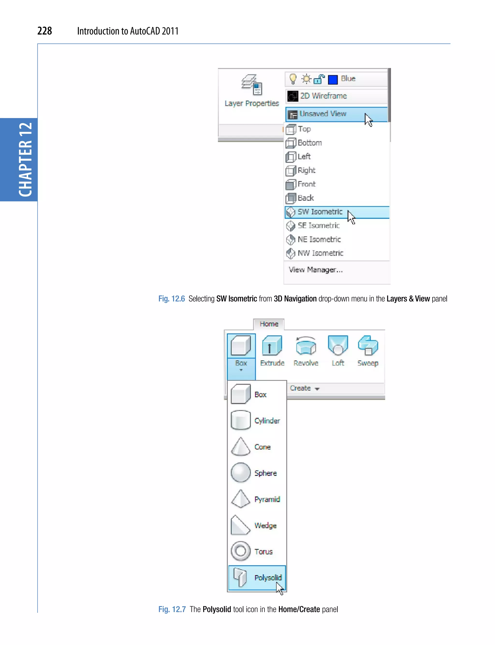
![Introducing 3D modeling 229
Specify start point or [Object/Height/Width/
Justify] <Object>: pick the polygon
Select object: right-click
Command:
chapter 12
And the Polysolid forms.
5. Select Conceptual from the Layers & View panel (Fig. 12.8).
The result is shown in Fig. 12.9.
Fig. 12.9 The Polysolid
tool example
Fig. 12.8 Selecting Conceptual shading from Visual Styles in the Layers & View panel
2D outlines suitable for 3D models
When constructing 2D outlines suitable as a basis for constructing some
forms of 3D model, select a tool from the Home/Draw panel, or enter tool
names or abbreviations for the tools at the command line. If constructed
using tools such as Line, Circle and Ellipse, before being of any use for
3D modeling, outlines must be changed into regions with the Region tool.
Closed polylines can be used without the need to use the Region tool.](https://image.slidesharecdn.com/introductiontoautocad2011-100614022653-phpapp02/75/Introduction-to-AutoCad-2011-223-2048.jpg)
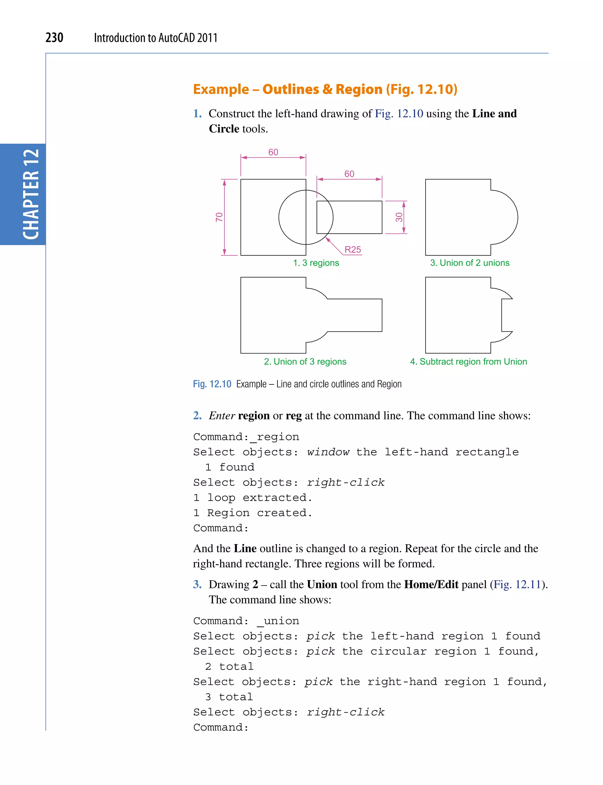
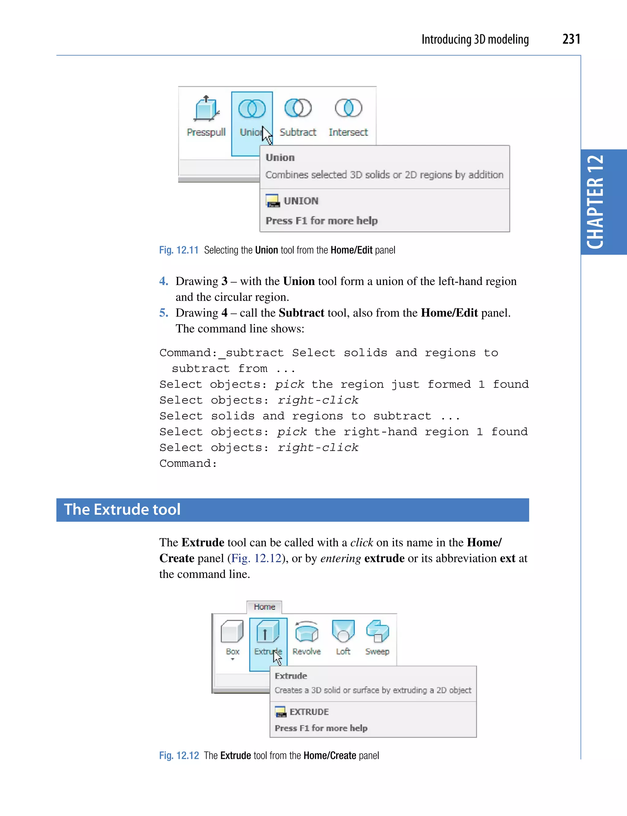
![232 Introduction to AutoCAD 2011
Examples of the use of the Extrude tool
The first two examples of forming regions given in Figs 12.10 and 12.11
are used to show the results of using the Extrude tool.
chapter 12
First example – Extrude (Fig. 12.13)
From the first example of forming a region:
1. Open Fig. 12.10. Erase all but the region 2.
2. Make layer Green current.
3. Call Extrude (Fig. 12.12). The command line shows:
Command: _extrude
Current wire frame density: ISOLINES=4
Closed profiles creation mode=Solid
Select objects to extrude or [MOde]: pick region
1 found
Select objects to extrude or [MOde]: right click
Specify height of extrusion or [Direction/Path/
Taper angle/Expression] <45>: enter 50 right-
click
Command:
4. Place in the Layers & View/3D Navigation/SW/Isometric view.
5. Call Zoom and zoom to 1.
6. Place in Visual Style/Realistic.
The result is shown in Fig. 12.13.
Fig. 12.13 First example – Extrude](https://image.slidesharecdn.com/introductiontoautocad2011-100614022653-phpapp02/75/Introduction-to-AutoCad-2011-226-2048.jpg)
![Introducing 3D modeling 233
Notes
1. In the above example we made use of an isometric view possible
from the 3D Navigation drop-down menu in the Home/Layers &
Views panel (Fig. 12.6). The 3D Navigation drop-down menu
chapter 12
allows a model to be shown in a variety of views.
2. Note the Current wire frame density: ISOLINES4 in the
prompts sequence when Extrude is called. The setting of 4 is
suitable when extruding plines or regions consisting of straight lines,
but when arcs are being extruded it may be better to set ISOLINES
to a higher figure as follows:
Command: enter isolines right-click
Enter new value for ISOLINES <4>: enter 16
right-click
Command:
3. Note the prompt [MOde] in the line
Select objects to extrude or [MOde]:
If mo is entered as a response to this prompt line, the following prompts
appear:
Closed profiles creation mode[SOlid/SUrface]
<Solid>: _SO
which allows the extrusion to be in solid or surface format.
Second example – Extrude (Fig. 12.14)
1. Open Fig. 12.10 and erase all but the region 3.
2. Make the layer Blue current.
3. Set ISOLINES to 16.
4. Call the Extrude tool. The command line shows:
Command: _extrude
Current wire frame density: ISOLINES=4, Closed
profiles creation mode=Solid
Select objects to extrude or [MOde]: _MO Closed
profiles creation mode
[SOlid/SUrface] <Solid>: _SO
Select objects to extrude or [MOde]: pick the
region 3 1 found
Select objects to extrude or [MOde]:](https://image.slidesharecdn.com/introductiontoautocad2011-100614022653-phpapp02/75/Introduction-to-AutoCad-2011-227-2048.jpg)
![234 Introduction to AutoCAD 2011
Specify height of extrusion or [Direction/Path/
Taper angle/Expression]: enter t right-click
Specify angle of taper for extrusion or
[Expression] <0>: enter 10 right-click
Specify height of extrusion or [Direction/Path/
chapter 12
Taper angle/Expression]: enter 100 right-click
Command:
3. In the Layers & View/3D Navigation menu select NE Isometric.
4. Zoom to 1.
5. Place in Visual Styles/Hidden.
Fig. 12.14 Second
example – Extrude The result is shown in Fig. 12.14.
Third example – Extrude (Fig. 12.16)
1. Make layer Magnolia current.
2. Construct an 80 50 rectangle, filleted to a radius of 15. Then in
the 3D Navigation/Front view and using the 3D Polyline tool from
the Home/Draw panel (Fig. 12.15), construct 3 3D polylines each of
length 45 and at 45 degree to each other at the centre of the outline as
shown in Fig. 12.16.
3. Place the screen in the 3D Navigation/SW Isometric view.
4. Set ISOLINES to 24.
5. Call the Extrude tool. The command line shows:
Command: _extrude
Current wire frame density: ISOLINES = 24, Closed
profiles creation mode = Solid
Select objects to extrude or [MOde]: _MO Closed
profiles creation mode
[SOlid/SUrface] <Solid>: _SO
Select objects to extrude or [MOde]: pick the
rectangle 1 found
Select objects to extrude or [MOde]: right-click
Specify height of extrusion or [Direction/Path/
Taper angle/Expression]:enter t right-click
Select extrusion path or [Taper angle]: pick path
right-click
Command:
Fig. 12.15 The 3D 6. Place the model in Visual Styles/Realistic.
Polyline tool from the
Home/Draw panel The result is shown in Fig. 12.16.](https://image.slidesharecdn.com/introductiontoautocad2011-100614022653-phpapp02/75/Introduction-to-AutoCad-2011-228-2048.jpg)
![Introducing 3D modeling 235
Path
Object
chapter 12
Fig. 12.16 Second example – Extrude
the revolve tool
The Revolve tool can be called with a click on its tool icon in the Home/
Create panel, by a click or by entering revolve at the command line, or its
abbreviation rev.
Examples of the use of the Revolve tool
Solids of revolution can be constructed from closed plines or from regions.
First example – Revolve (Fig. 12.19)
1. Construct the closed polyline (Fig. 12.17).
2. Make layer Red current.
3. Set ISOLINES to 24.
4. Call the Revolve tool from the Home/Create panel (Fig. 12.18).
The command line shows:
Command: _revolve
Current wire frame density: ISOLINES=4, Closed
profiles creation mode=Solid
Select objects to revolve or [MOde]: _MO Closed
profiles creation mode[SOlid/SUrface] <Solid>: _SO
10 85 R10
R5
45
45
10
15
Start point for axis 280 Axis endpoint
Fig. 12.17 First example – Revolve. The closed pline](https://image.slidesharecdn.com/introductiontoautocad2011-100614022653-phpapp02/75/Introduction-to-AutoCad-2011-229-2048.jpg)
![chapter 12 236 Introduction to AutoCAD 2011
Fig. 12.18 The Revolve tool from the Home/Create panel
Select objects to revolve or [MOde]: pick the
pline 1 found
Select objects to revolve or [MOde]: right-click
Specify axis start point or define axis by [Object/
X/Y/Z] <Object>: pick
Specify axis endpoint: pick
Specify angle of revolution or [STart angle/
Reverse/Expression] <360>: right-click
Command:
5. Place in the 3D Navigation/NE Isometric view. Zoom to 1.
6. Shade with Visual Styles/Shaded.
Fig. 12.19 First
example – Revolve The result is shown in Fig. 12.19.
Second example – Revolve (Fig. 12.21)
1. Make layer Yellow current.
2. Place the screen in the 3D Navigate/Front view. Zoom to 1.
3. Construct the pline outline (Fig. 12.20).
4
4
40
Semi-ellipse based
on 180 x 100 axes
Fig. 12.20 Second example – Revolve. The pline outline](https://image.slidesharecdn.com/introductiontoautocad2011-100614022653-phpapp02/75/Introduction-to-AutoCad-2011-230-2048.jpg)
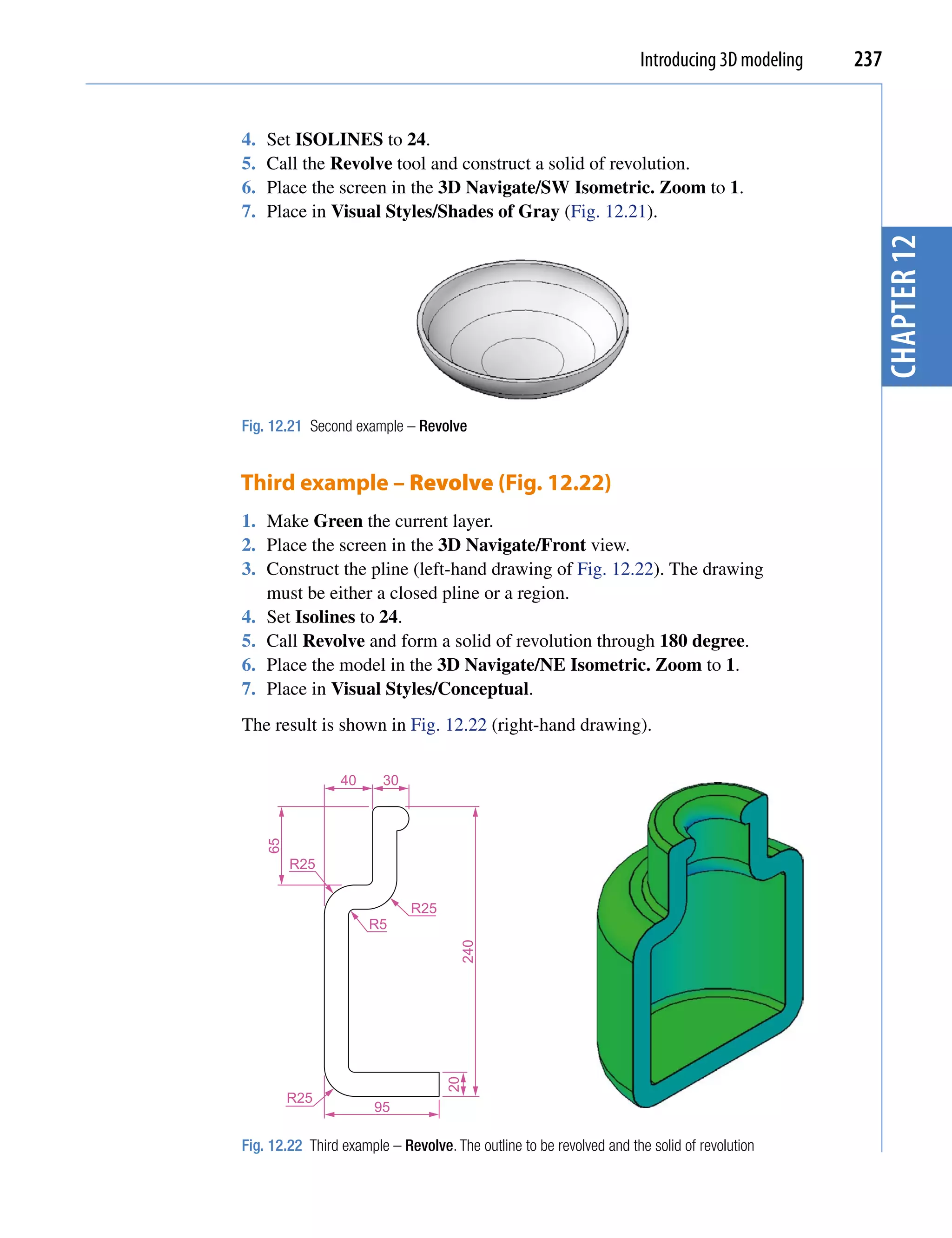
![238 Introduction to AutoCAD 2011
other tools from the home/create panel
First example – Box (Fig. 12.24)
1. Make Magenta the current layer.
chapter 12
2. Place the window in the 3D Navigate/Front view.
3. Set Isolines to 4.
4. Click the Box tool icon in the Home/Create panel (Fig. 12.23). The
command line shows:
Command: _box
Specify first corner or [Center]: enter 90,90
right-click
Specify other corner or [Cube/Length]: enter 110,
-30 right-click
Specify height or [2Point]: enter 75 right-click
Command: right-click
BOX Specify first corner or [Center]: 110,90
Specify other corner or [Cube/Length]: 170,70
Specify height or [2Point]: 75
Command:
Fig. 12.23 Selecting
BOX Specify first corner or [Center]: 110,-10
Box from the Home/ Specify other corner or [Cube/Length]: 200,-30
Create panel Specify height or [2Point]: 75
Command:
5. Place in the ViewCube/Isometric view. Zoom to 1.
6. Call the Union tool from the Home/Edit panel. The command line
shows:
Command:_union
Select objects: pick one of the boxes 1 found
Select objects: pick the second of box 1 found,
2 total
Select objects: pick the third box 1 found,
3 total
Select objects: right-click
Command:
And the three boxes are joined in a single union.
7. Place in Visual Styles/Conceptual.
Fig. 12.24 First
example – Box The result is given in Fig. 12.24.](https://image.slidesharecdn.com/introductiontoautocad2011-100614022653-phpapp02/75/Introduction-to-AutoCad-2011-232-2048.jpg)
![Introducing 3D modeling 239
Second example – Sphere and Cylinder (Fig. 12.25)
1. Make layer Green current.
2. Set ISOLINES to 16.
3. Click the Sphere tool icon from the Home/Create panel. The command
chapter 12
line shows:
Command: _sphere
Specify center point or [3P/2P/Ttr]: 180,170
Specify radius or [Diameter]: 50
Command:
4. Click the Cylinder tool icon in the Home/Create panel. The command
line shows:
Command: _cylinder
Specify center point of base or [3P/2P/Ttr/
Elliptical]: 180,170
Specify base radius or [Diameter]: 25
Specify height or [2Point/Axis endpoint]: 110
Command:
5. Place the screen in the 3D Navigate/Front view. Zoom to 1.
6. With the Move tool (from the Home/Modify panel), move the cylinder
vertically down so that the bottom of the cylinder is at the bottom of the
sphere.
7. Click the Subtract tool icon in the Home/Edit panel. The command
line shows:
Command: _subtract Select solids and regions to
subtract from...
Select objects: pick the sphere 1 found
Select objects: right-click
Select solids and regions to subtract
Select objects: pick the cylinder 1 found
Select objects: right-click
Command:
8. Place the screen in 3D Navigate/SW Isometric. Zoom to 1.
Fig. 12.25 Second 9. Place in Visual Styles/Realistic.
example – Sphere and
Cylinder The result is shown in Fig. 12.25.
Third example – Cylinder, Cone and Sphere (Fig. 12.26)
1. Make Blue the current layer.
2. Set Isolines to 24.](https://image.slidesharecdn.com/introductiontoautocad2011-100614022653-phpapp02/75/Introduction-to-AutoCad-2011-233-2048.jpg)
![240 Introduction to AutoCAD 2011
3. Place in the 3D Navigate/Front view.
4. Call the Cylinder tool and with a centre 170,150 construct a cylinder
of radius 60 and height 15.
5. Click the Cone tool in the Home/Create panel. The command line
shows:
chapter 12
Command: _cone
Specify center point of base or [3P/2P/Ttr/
Elliptical]: 170,150
Specify base radius or [Diameter]: 40
Specify height or [2Point/Axis endpoint/Top
radius]: 150
Command:
6. Call the Sphere tool and construct a sphere of centre 170,150 and
radius 45.
7. Place the screen in the 3D Navigate/Front view and with the Move
tool, move the cone and sphere so that the cone is resting on the
cylinder and the centre of the sphere is at the apex of the cone.
8. Place in the 3D Navigate/SW Isometric view, Zoom to 1 and with
Union form a single 3D model from the three objects.
Fig. 12.26 Third 9. Place in Visual Styles/Conceptual.
example – Cylinder,
Cone and Sphere The result is shown in Fig. 12.26.
Fourth example – Box and Wedge (Fig. 12.27)
1. Make layer Blue current.
2. Place in the 3D Navigate/Top view.
3. Click the Box tool icon in the Home/Create panel and construct
two boxes, the first from corners 70,210 and 290,120 of height 10,
the second of corners 120,200,10 and 240,120,10 and of height 80.
4. Place the screen in the 3D Navigate/Front view and Zoom to 1.
5. Click the Wedge tool icon in the Home/Create panel. The command
line shows:
Command: _wedge
Specify first corner or [Center]: 120,170,10
Specify other corner or [Cube/Length]:
80,160,10
Specify height or [2Point]: 70
Command: right-click
WEDGE
Specify first corner of wedge or [Center]:
240,170,10](https://image.slidesharecdn.com/introductiontoautocad2011-100614022653-phpapp02/75/Introduction-to-AutoCad-2011-234-2048.jpg)
![Introducing 3D modeling 241
Specify corner or [Cube/Length]: 280,160,10
Specify height or [2Point]: 70
Command:
6. Place the screen in 3D Navigate/SW Isometric and Zoom to 1.
chapter 12
7. Call the Union tool from the Home/Edit panel and in response to the
prompts in the tool’s sequences pick each of the 4 objects in turn to
form a union of the 4 objects.
Fig. 12.27 Fourth 8. Place in Visual Styles/Conceptual.
example – Box and
Wedge The result is shown in Fig. 12.27.
Fifth example – Cylinder and Torus (Fig. 12.28)
1. Make layer Red current.
2. Set Isolines to 24.
3. Using the Cylinder tool from the Home/Create panel, construct a
cylinder of centre 180,160, of radius 40 and height 120.
4. Click the Torus tool icon in the Home/Create panel. The command
line shows:
Command: _torus
Specify center point or [3P/2P/Ttr]:
180,160,10
Specify radius or [Diameter]: 40
Specify tube radius or [2Point/Diameter]: 10
Command: right-click
TORUS
Specify center point or [3P/2P/Ttr]:
180,160,110
Specify radius or [Diameter] <40>: right-click
Specify tube radius or [2Point/Diameter] <10>:
right-click
Command:
5. Call the Cylinder tool again and construct another cylinder of centre
180, 160, of radius 35 and height 120.
6. Place in the 3D Navigate/SW Isometric view and Zoom to 1.
7. Click the Union tool icon in the Home/Edit panel and form a union of
the larger cylinder and the two torii.
8. Click the Subtract tool icon in the Home/Edit panel and subtract the
smaller cylinder from the union.
Fig. 12.28 Fifth 9. Place in Visual Styles/X-Ray.
example – Cylinder
and Torus The result is shown in Fig. 12.28.](https://image.slidesharecdn.com/introductiontoautocad2011-100614022653-phpapp02/75/Introduction-to-AutoCad-2011-235-2048.jpg)
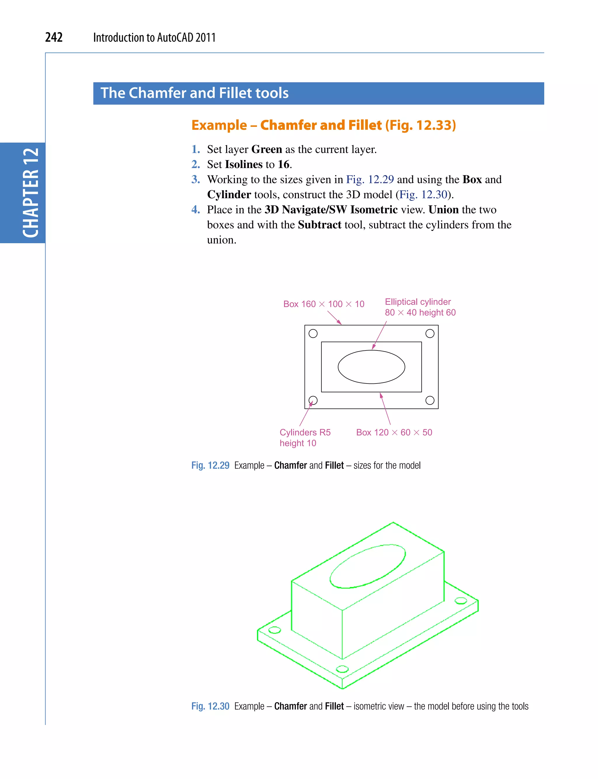
![Introducing 3D modeling 243
Notes
To construct the elliptical cylinder, call the Cylinder tool from the
Home/Modeling panel. The command line shows:
chapter 12
Command: _cylinder
Specify center point of base or [3P/2P/Ttr/
Elliptical]: enter e right-click
Specify endpoint of first axis or [Center]:
130,160
Specify other endpoint of first axis: 210,160
Specify endpoint of second axis: 170,180
Specify height or [2Point/Axis endpoint]: 50
Command:
5. Click the Fillet tool icon in the Home/Modify panel (Fig. 12.31).
The command line shows:
Fig. 12.31 The Fillet tool icon in the Home/Modify panel
Command:_fillet
Current settings: Mode=TRIM. Radius=0
Specify first object or [Undo/Polyline/Radius/
Trim/Multiple]: enter r (Radius) right-click
Specify fillet radius <0>: 10
Select first object: pick one corner
Select an edge or [Chain/Radius]: pick a second
corner](https://image.slidesharecdn.com/introductiontoautocad2011-100614022653-phpapp02/75/Introduction-to-AutoCad-2011-237-2048.jpg)
![244 Introduction to AutoCAD 2011
Select an edge or [Chain/Radius]: pick a third
corner
Select an edge or [Chain/Radius]: pick the
fourth corner
chapter 12
Select an edge or [Chain/Radius]: right-click
4 edge(s) selected for fillet.
Command:
6. Click the Chamfer tool in the Home/Modify panel (Fig. 12.32). The
command line shows:
Fig. 12.32 The Chamfer tool icon in the Home/Modify panel
Command: _chamfer
(TRIM mode) Current chamfer Dist1 = 0, Dist2 = 0
Select first line or [Undo/Polyline/Distance/
Angle/Trim/mEthod/Multiple]: enter d right-click
Specify first chamfer distance <0>: 10
Specify second chamfer distance <10>:
Select first line or [Undo/Polyline/Distance/
Angle/Trim/mEthod/Multiple]: pick one corner
One side of the box highlights
Base surface selection...
Enter surface selection option [Next/OK
(current)] <OK>: right-click
Specify base surface chamfer distance <10>:
right-click
Specify other surface chamfer distance <10>:
right-click
Select an edge or [Loop]: pick the edge
Select an edge or [Loop]: pick the second edge
Select an edge [or Loop]: right-click
Command:](https://image.slidesharecdn.com/introductiontoautocad2011-100614022653-phpapp02/75/Introduction-to-AutoCad-2011-238-2048.jpg)
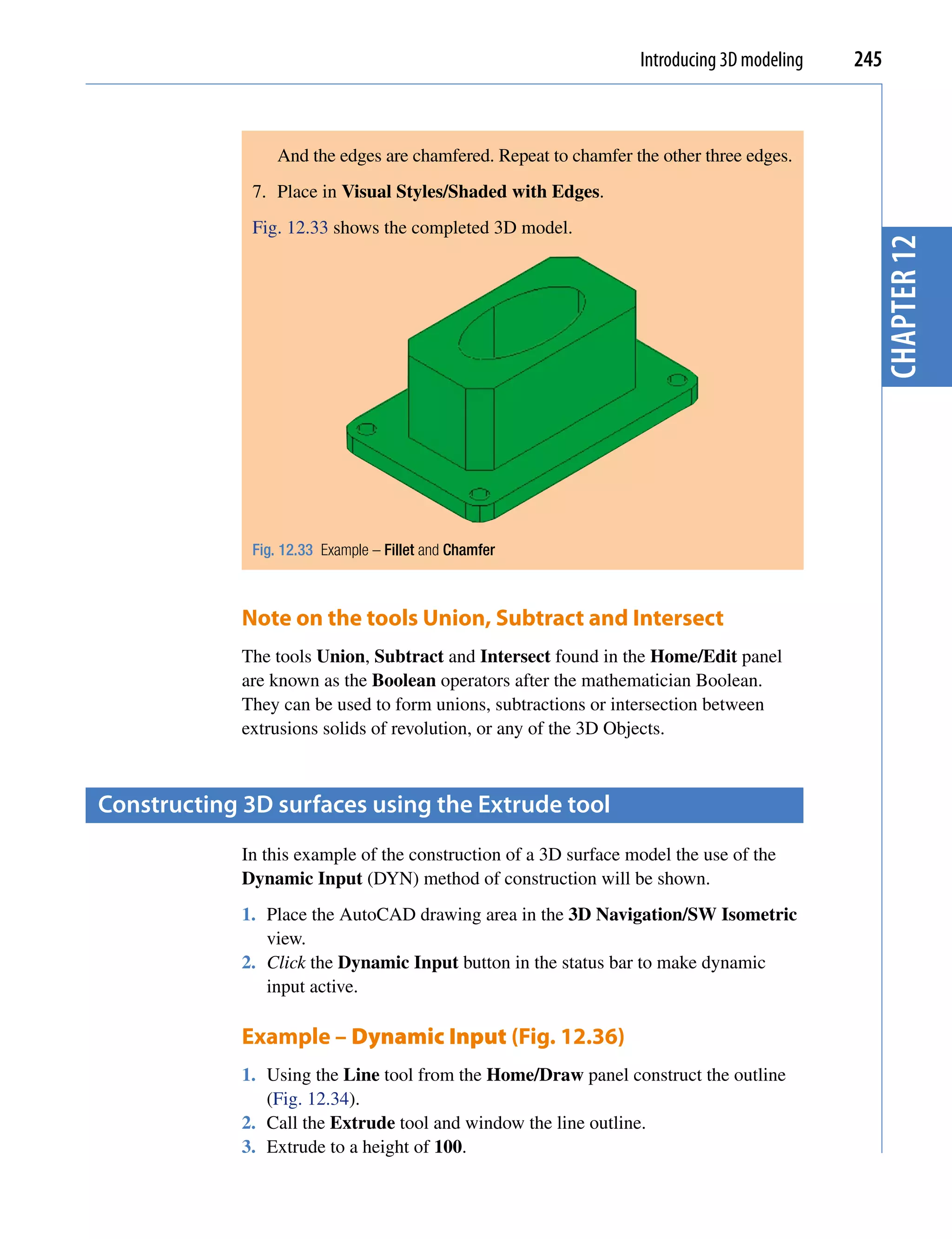
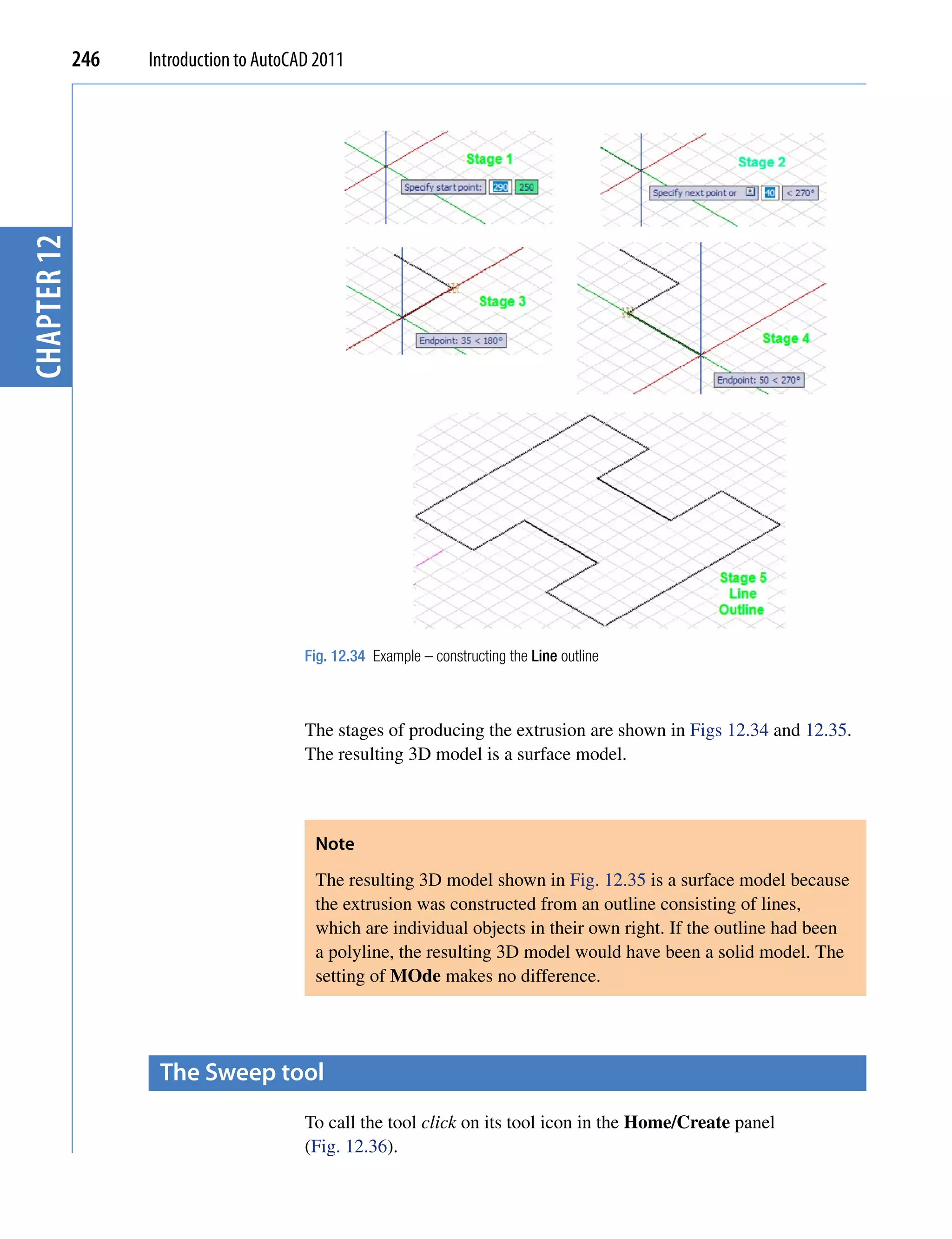
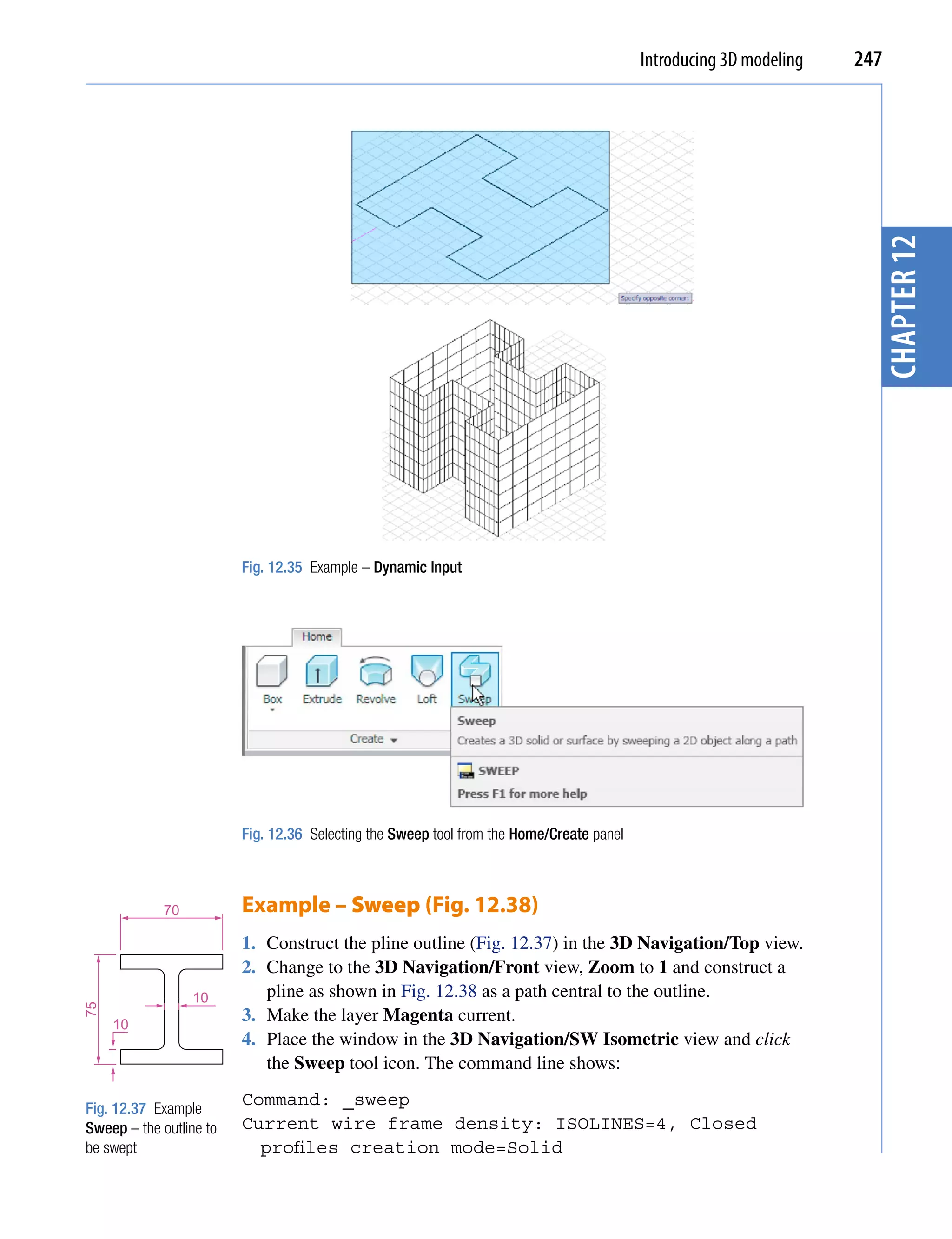
![248 Introduction to AutoCAD 2011
Select objects to sweep or [MOde]: _MO Closed
profiles creation mode
[SOlid/SUrface] <Solid>: _SO
Select objects to sweep or [MOde]: pick the pline
1 found
chapter 12
Select objects to sweep or [MOde]: right-click
Select sweep path or [Alignment/Base point/Scale/
Twist]: pick the pline path
Command:
5. Place in Visual Styles/Shaded.
The result is shown in Fig. 12.38.
R77
140
R94
130
Fig. 12.38 Example – Sweep
the Loft tool
To call the tool click on its icon in the Home/Create panel.
Example – Loft (Fig. 12.41)
1. In the 3D Navigate/Top view, construct the seven circles shown in
Fig. 12.39 at vertical distances of 30 units apart.
2. Place the drawing area in the 3D Navigate/SW Isometric view.
3. Call the Loft tool with a click on its tool icon in the Home/Modeling
panel (Fig. 12.40).](https://image.slidesharecdn.com/introductiontoautocad2011-100614022653-phpapp02/75/Introduction-to-AutoCad-2011-242-2048.jpg)
![Introducing 3D modeling 249
Ø100
Ø80
chapter 12
Ø60
Ø30
Ø60
Ø80
Ø100
Fig. 12.39 Example Loft – the cross sections
Fig. 12.40 Selecting the Loft tool from the Home/Create panel
4. Set Cyan as the current layer.
5. The command line shows:
Command:_loft
Select cross sections in lofting order or
[POint/Join multiple curves]: pick 1 found
Select cross sections in lofting order or [POint/
Join multiple curves]: pick 1
found, 2 total
Select cross sections in lofting order or [POint/
Join multiple curves]: pick 1](https://image.slidesharecdn.com/introductiontoautocad2011-100614022653-phpapp02/75/Introduction-to-AutoCad-2011-243-2048.jpg)
![250 Introduction to AutoCAD 2011
found, 3 total
Select cross sections in lofting order or [POint/
Join multiple curves]: pick 1 found, 4 total
Select cross sections in lofting order or [POint/
Join multiple curves]: pick 1 found, 5 total
chapter 12
Select cross sections in lofting order or [POint/
Join multiple curves]: pick 1 found, 6 total
Select cross sections in lofting order or [POint/
Join multiple curves]: pick 1 found, 7 total
Select cross sections in lofting order or [POint/
Join multiple curves]: enter j right-click
Select curves that are to be joined into a single
cross section: right-click 7 cross sections
selected
Enter an option [Guides/Path/Cross sections only/
Settings] <Cross sections only>: right-click
Command:
6. Place in Visual Styles/Shaded with Edges.
Fig. 12.41 Example –
Loft The result is shown in Fig. 12.41.
REvISIoN NoTES
1. In the AutoCAD 3D coordinate system, positive Z is towards the operator away from the
monitor screen.
2. A 3D face is a mesh behind which other details can be hidden.
3. The Extrude tool can be used for extruding closed plines or regions to stated heights, to
stated slopes or along paths.
4. The Revolve tool can be used for constructing solids of revolution through any angle up to
360 degree.
5. 3D models can be constructed from Box, Sphere, Cylinder, Cone, Torus and Wedge.
Extrusions and/or solids of revolutions may form part of models constructed using these
3D tools.
6. The tools Union, Subtract and Intersect are known as the Boolean operators.
7. When polylines form an outline which is not closed are acted upon by the Extrude tool the
resulting models will be 3D Surface models irrespective of the MOde setting.](https://image.slidesharecdn.com/introductiontoautocad2011-100614022653-phpapp02/75/Introduction-to-AutoCad-2011-244-2048.jpg)
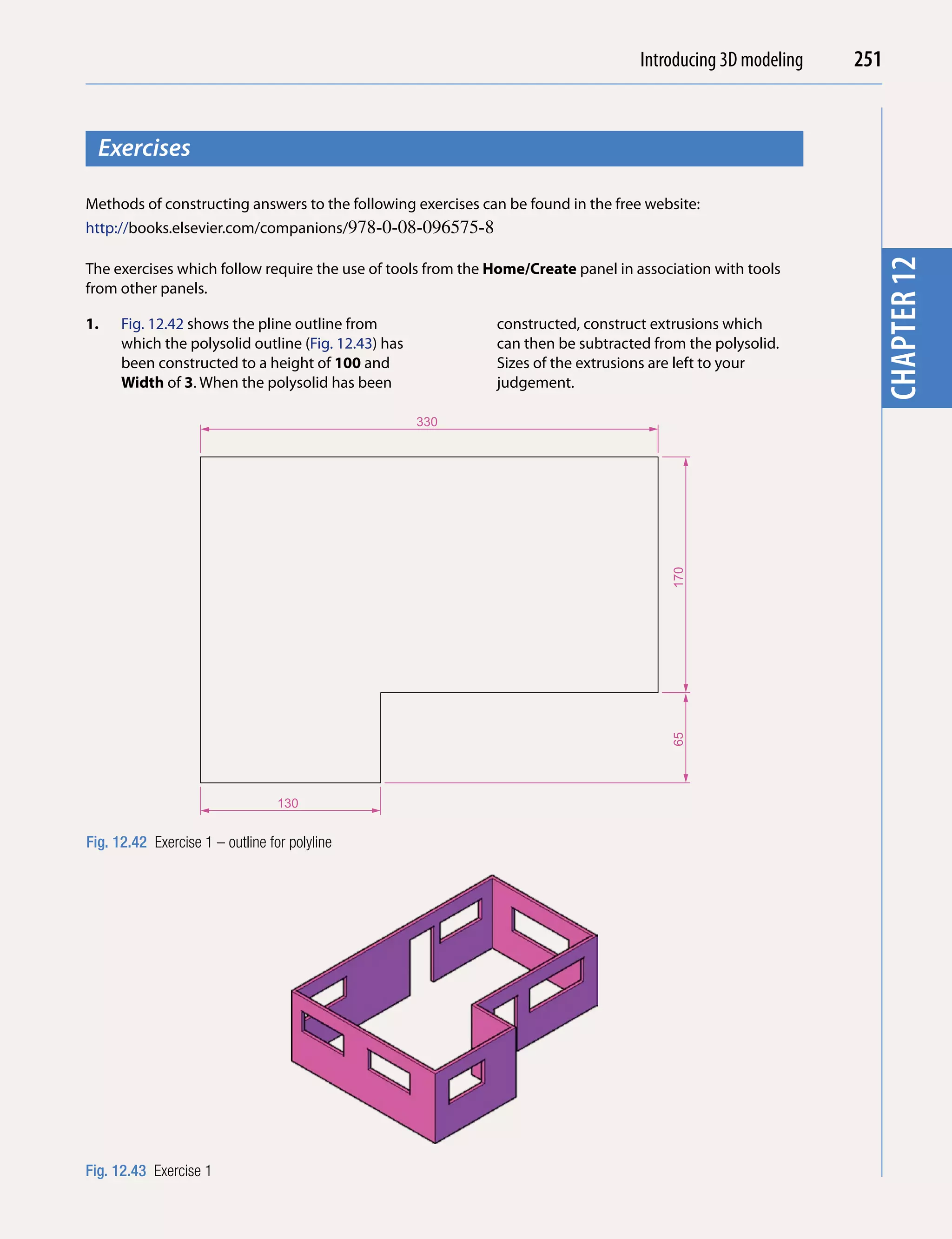
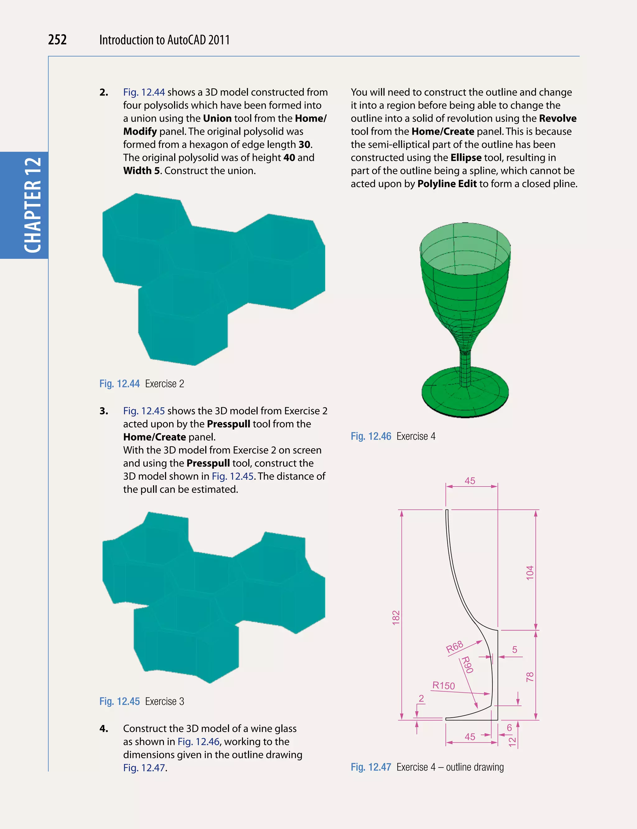
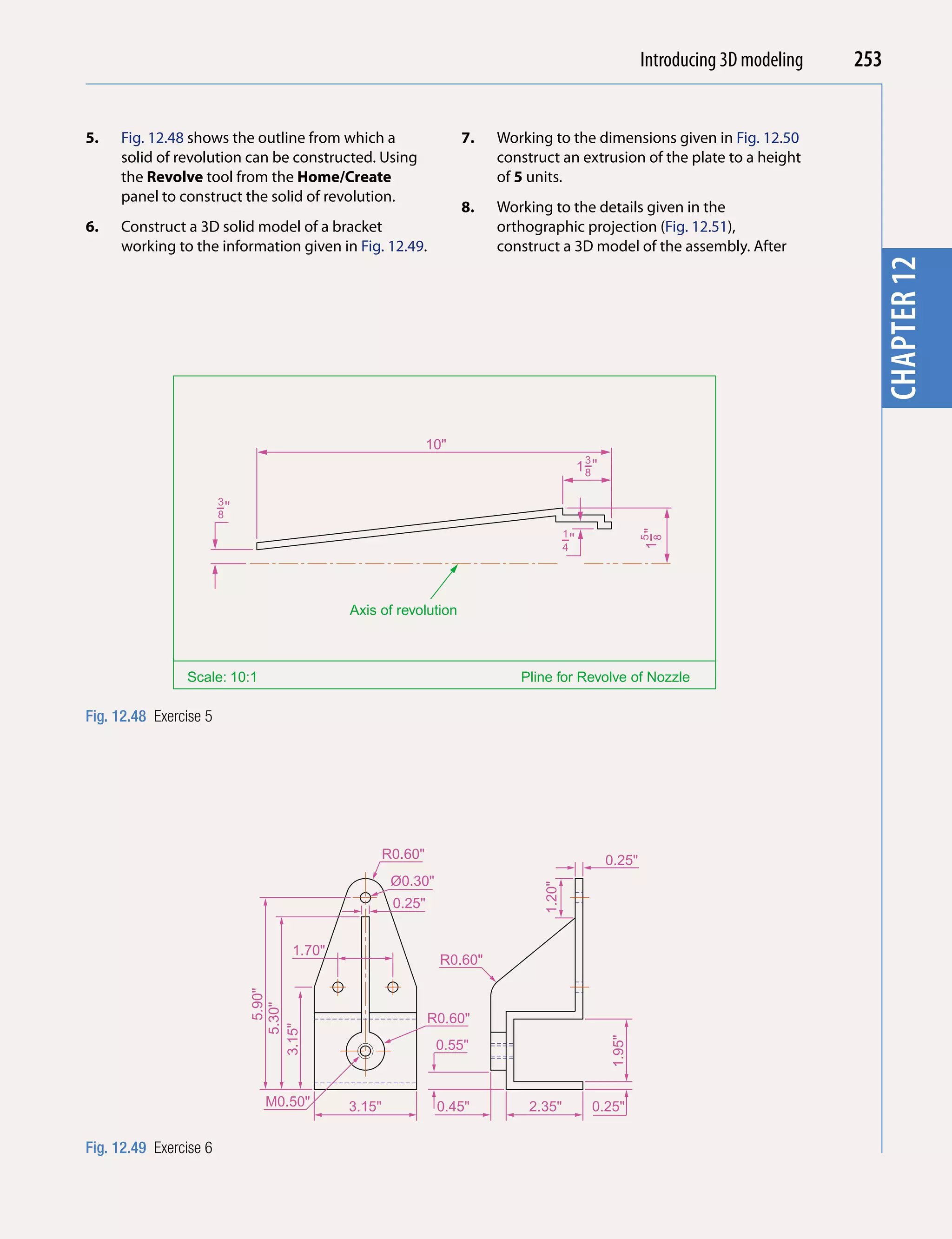
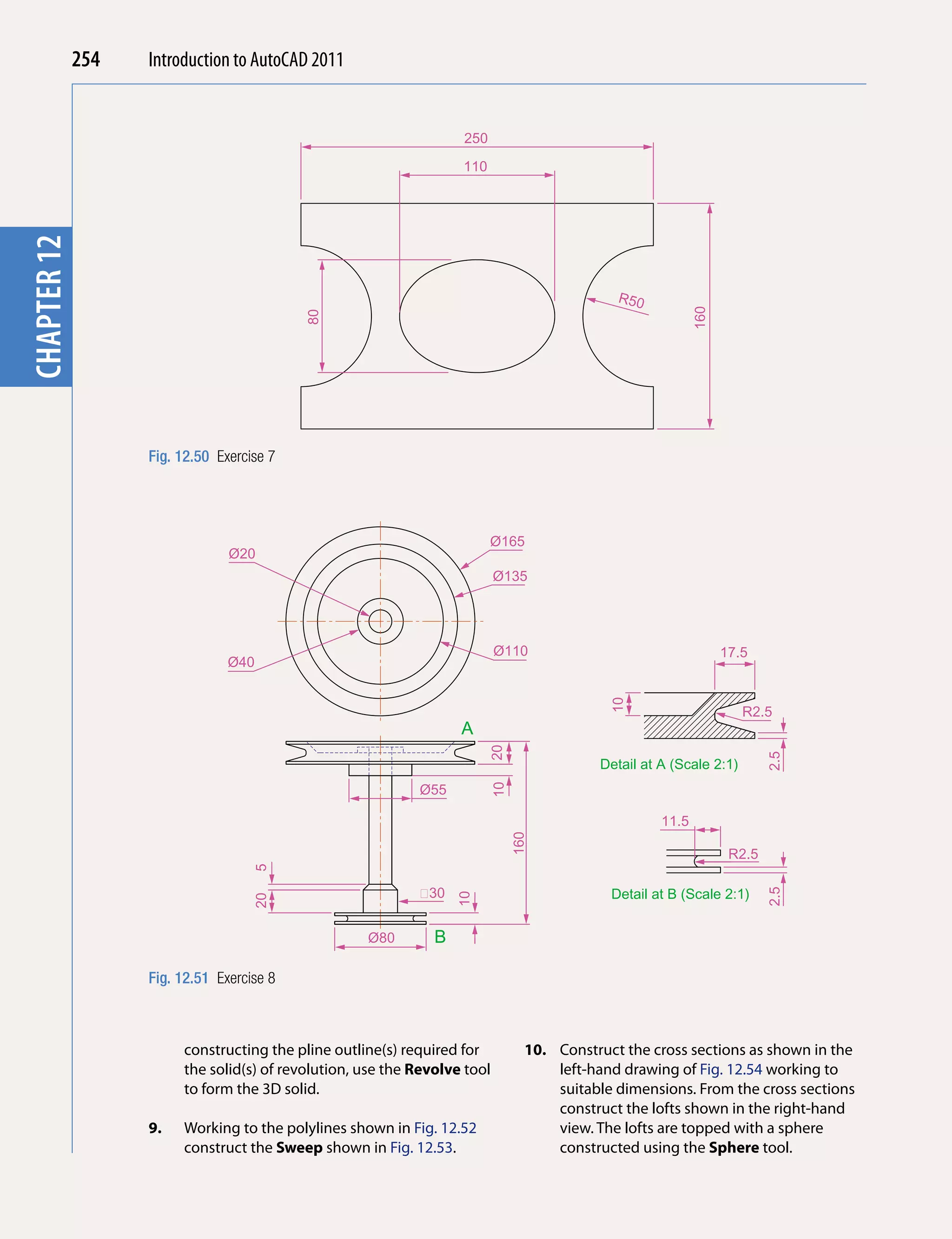
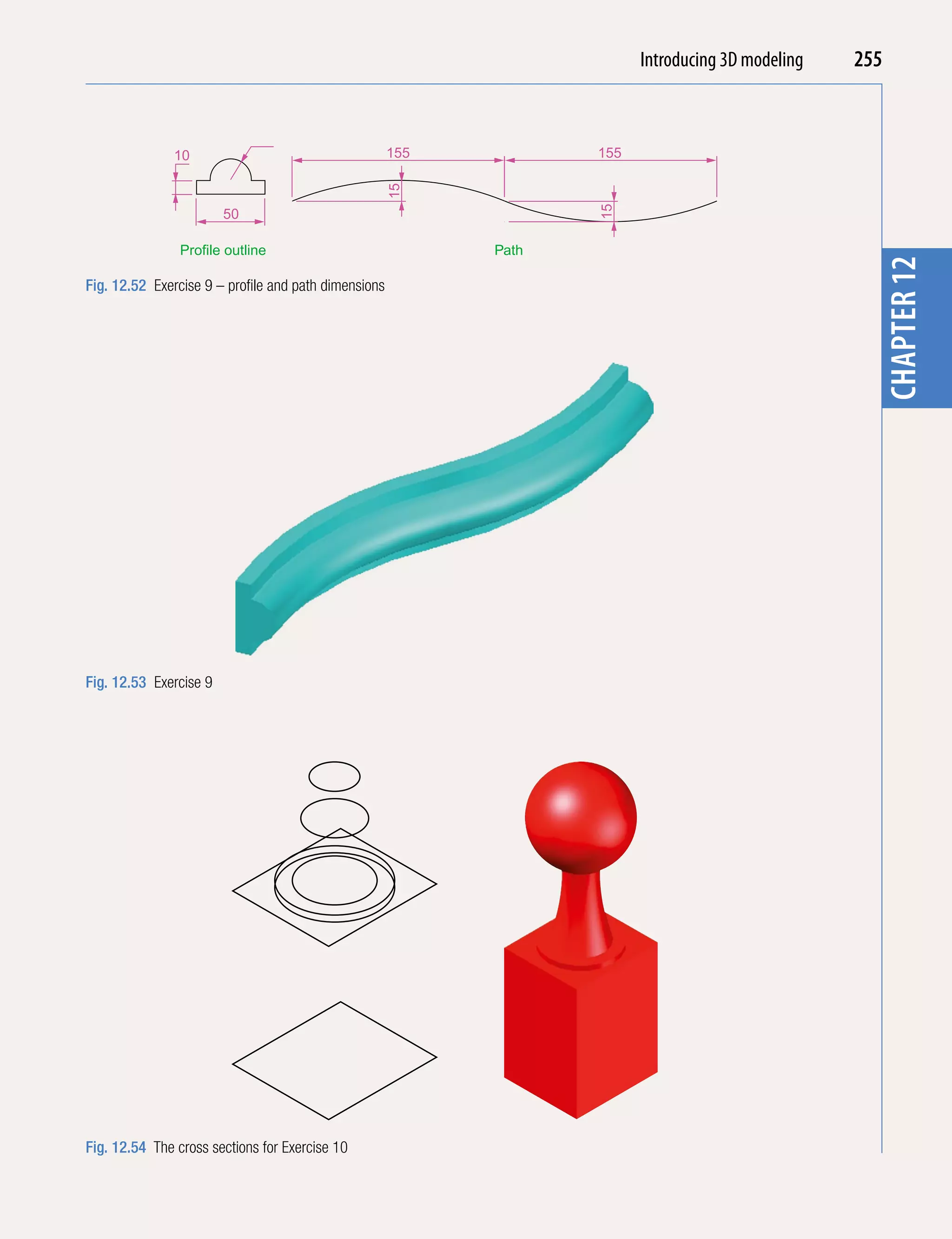
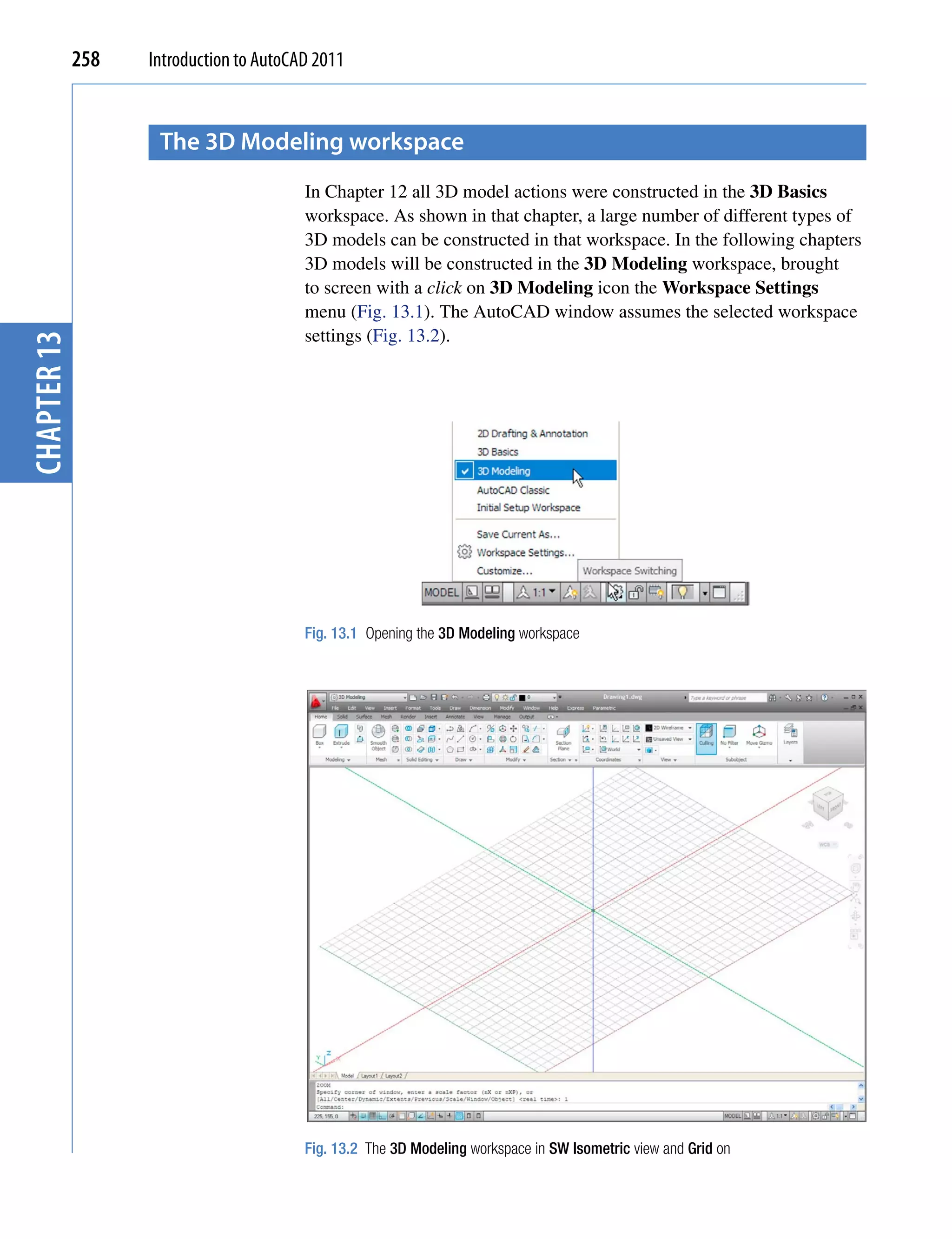
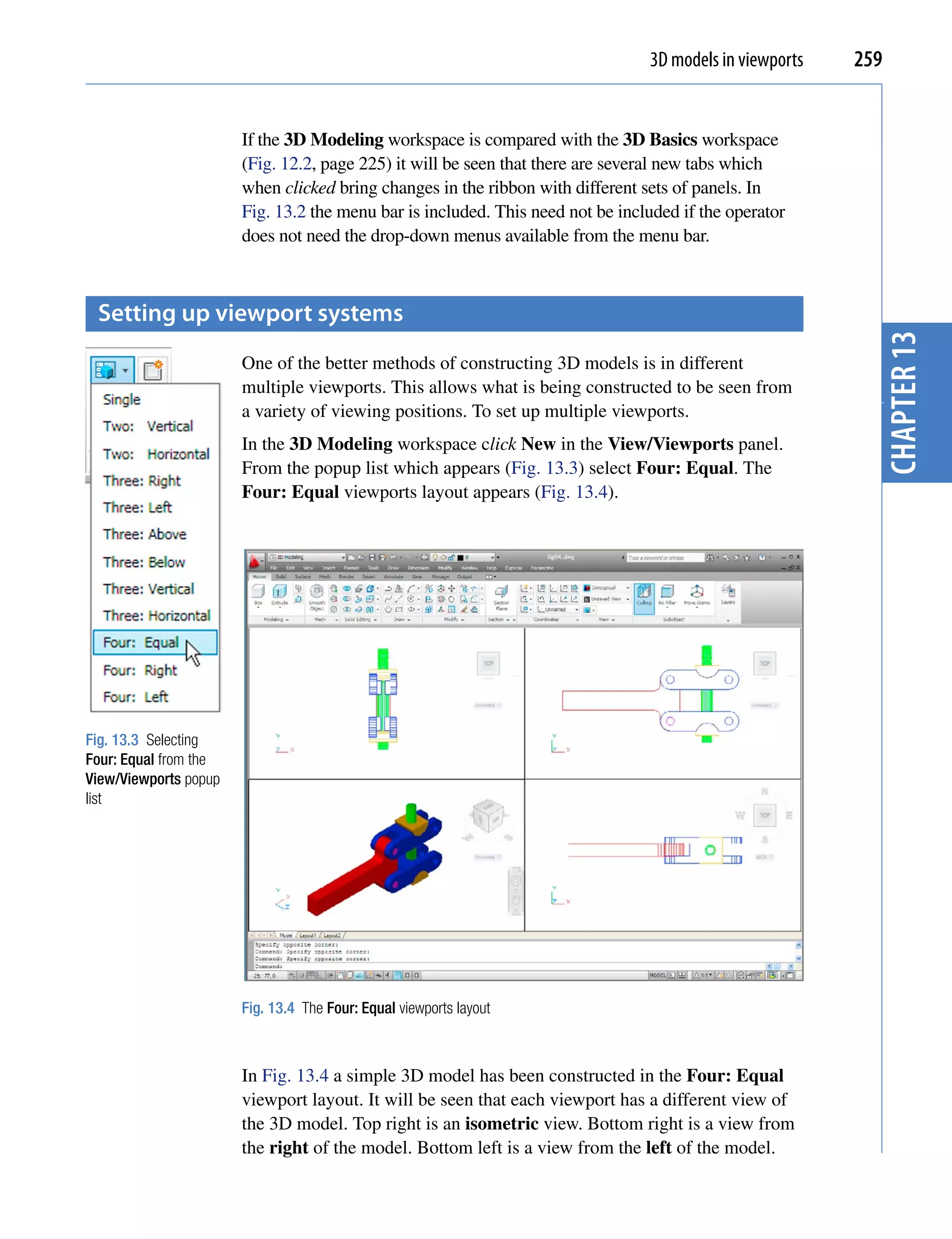
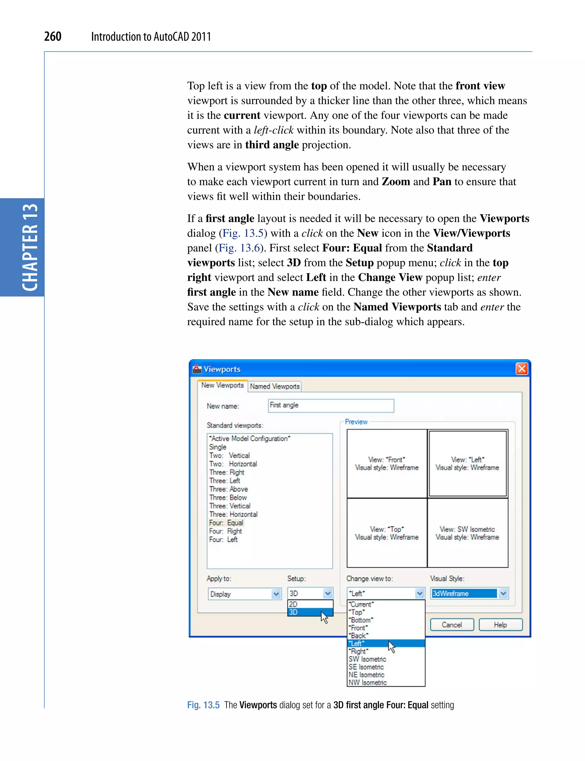
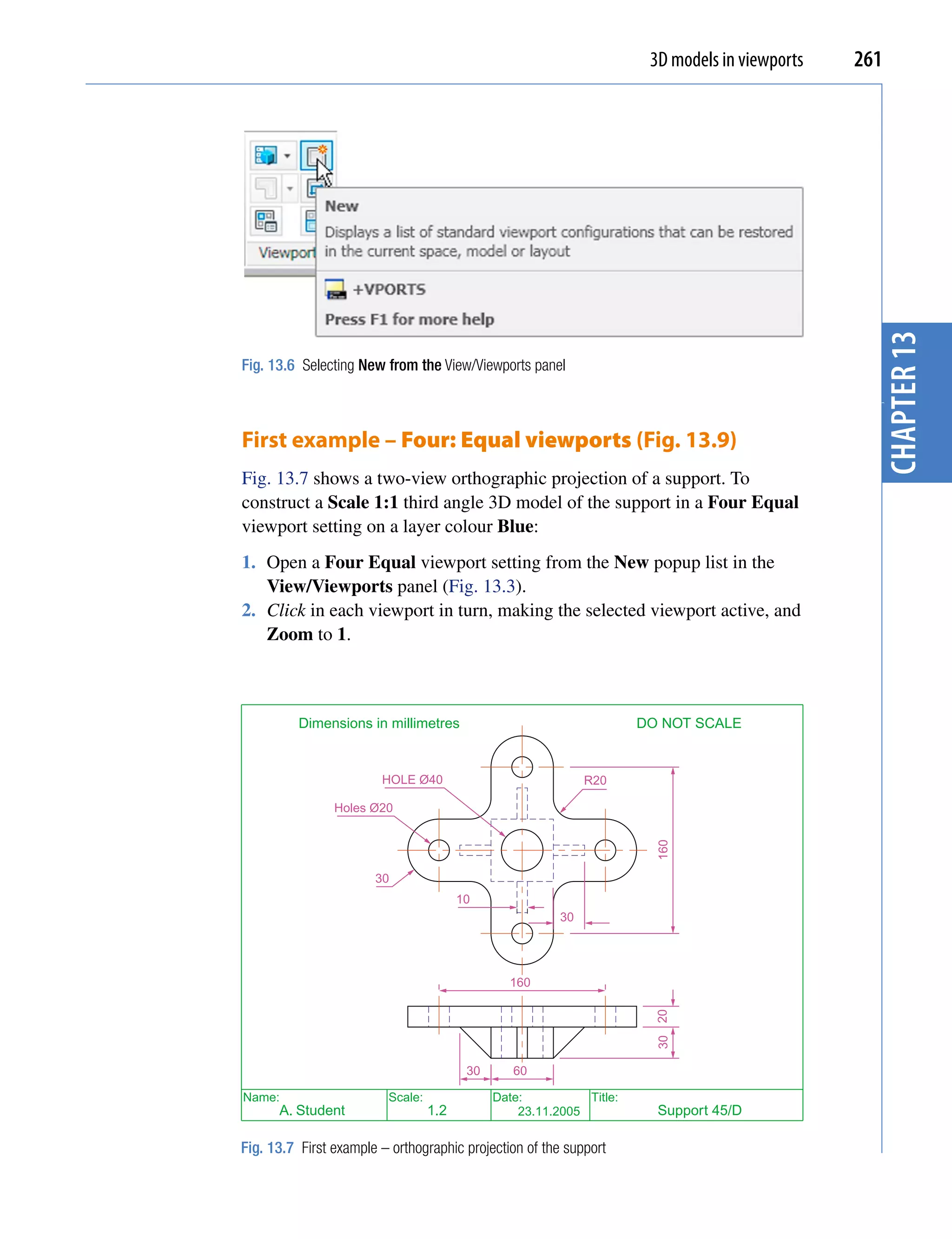
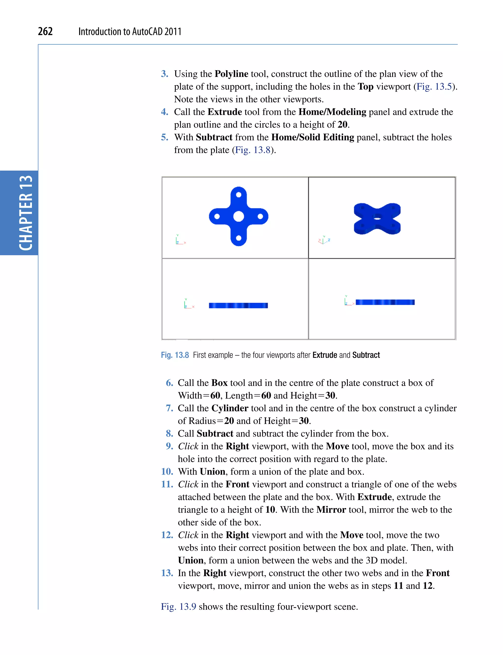
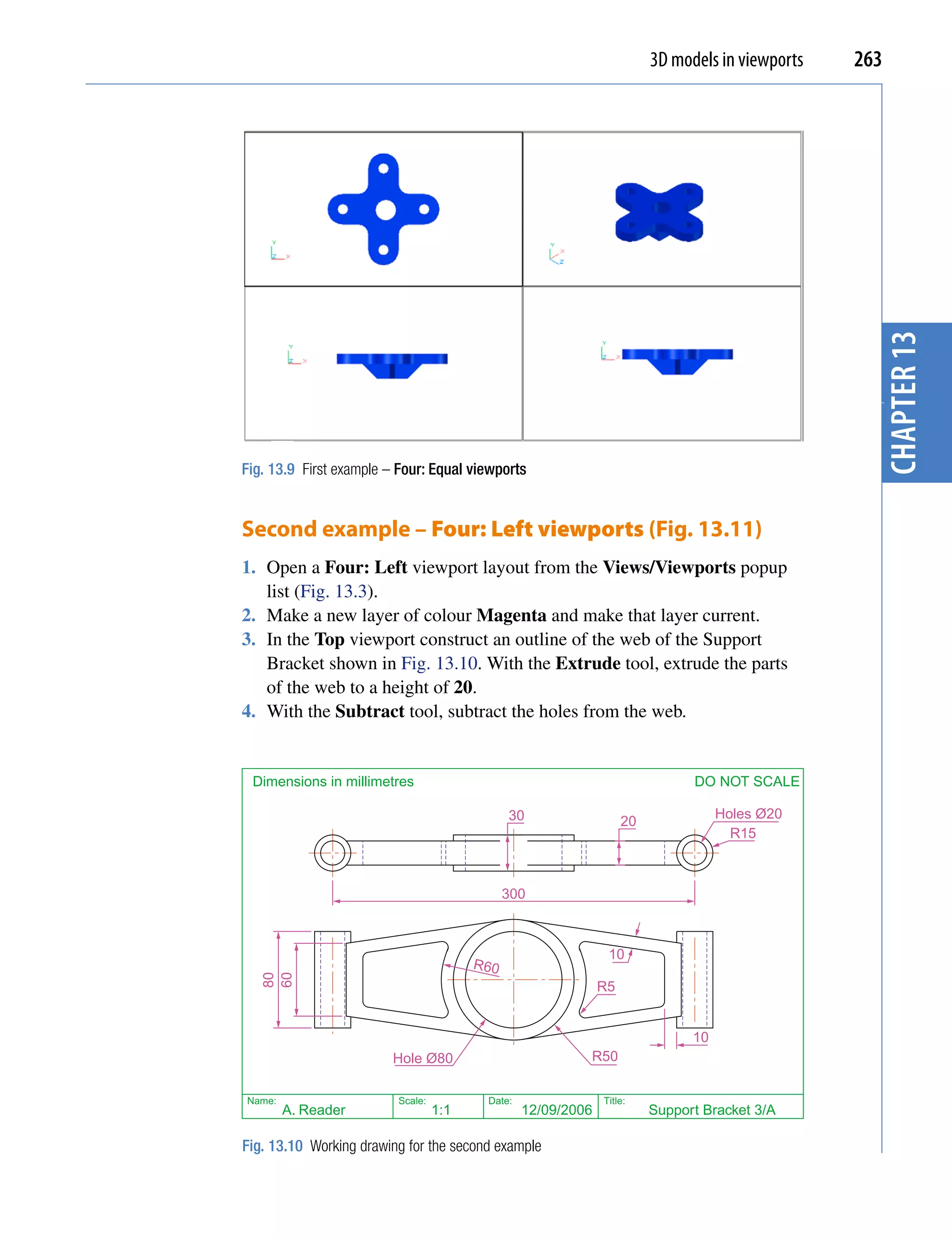
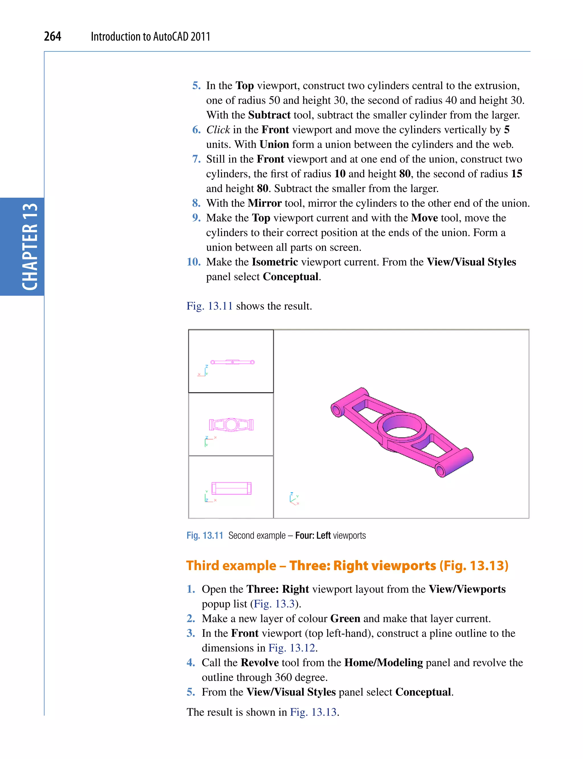
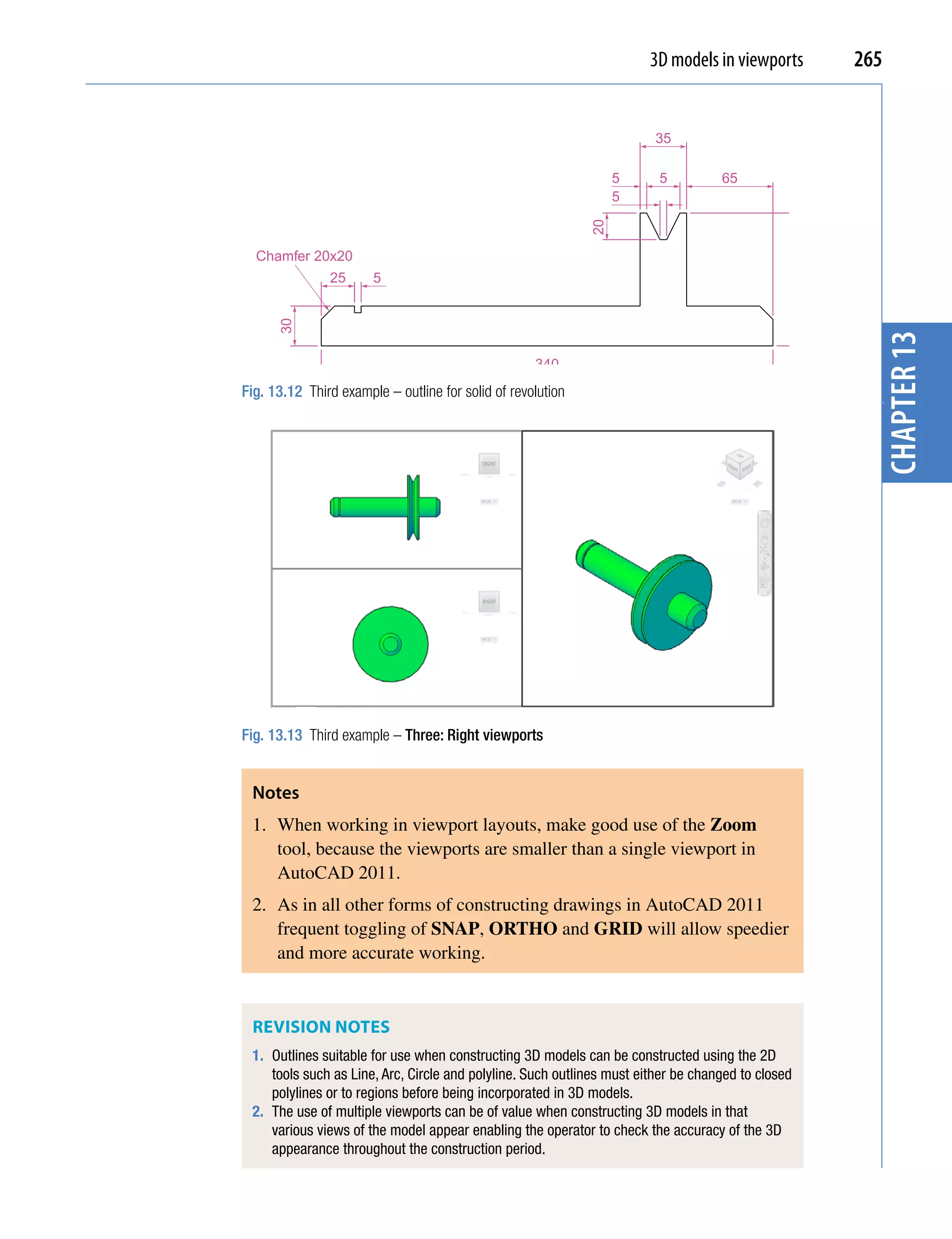
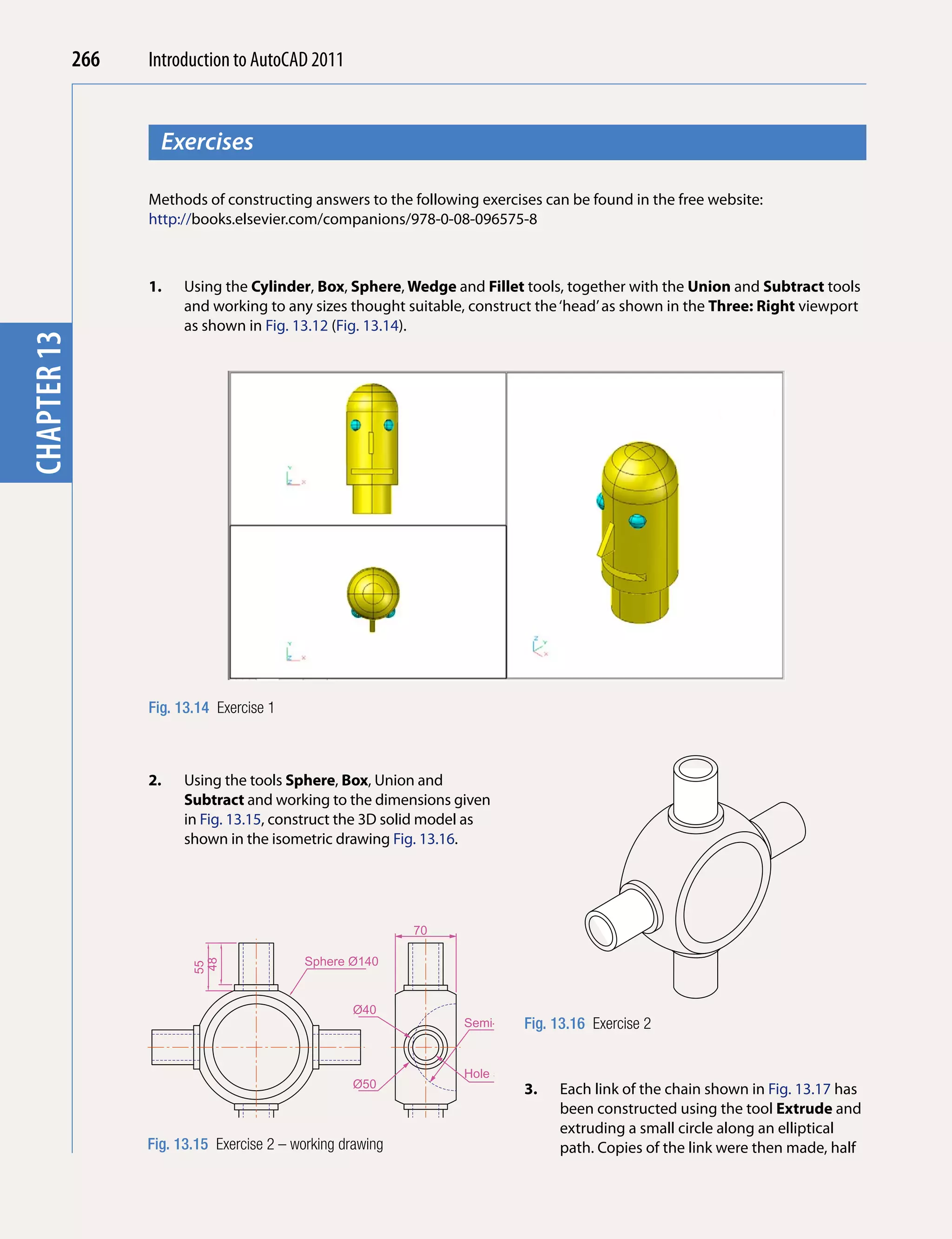
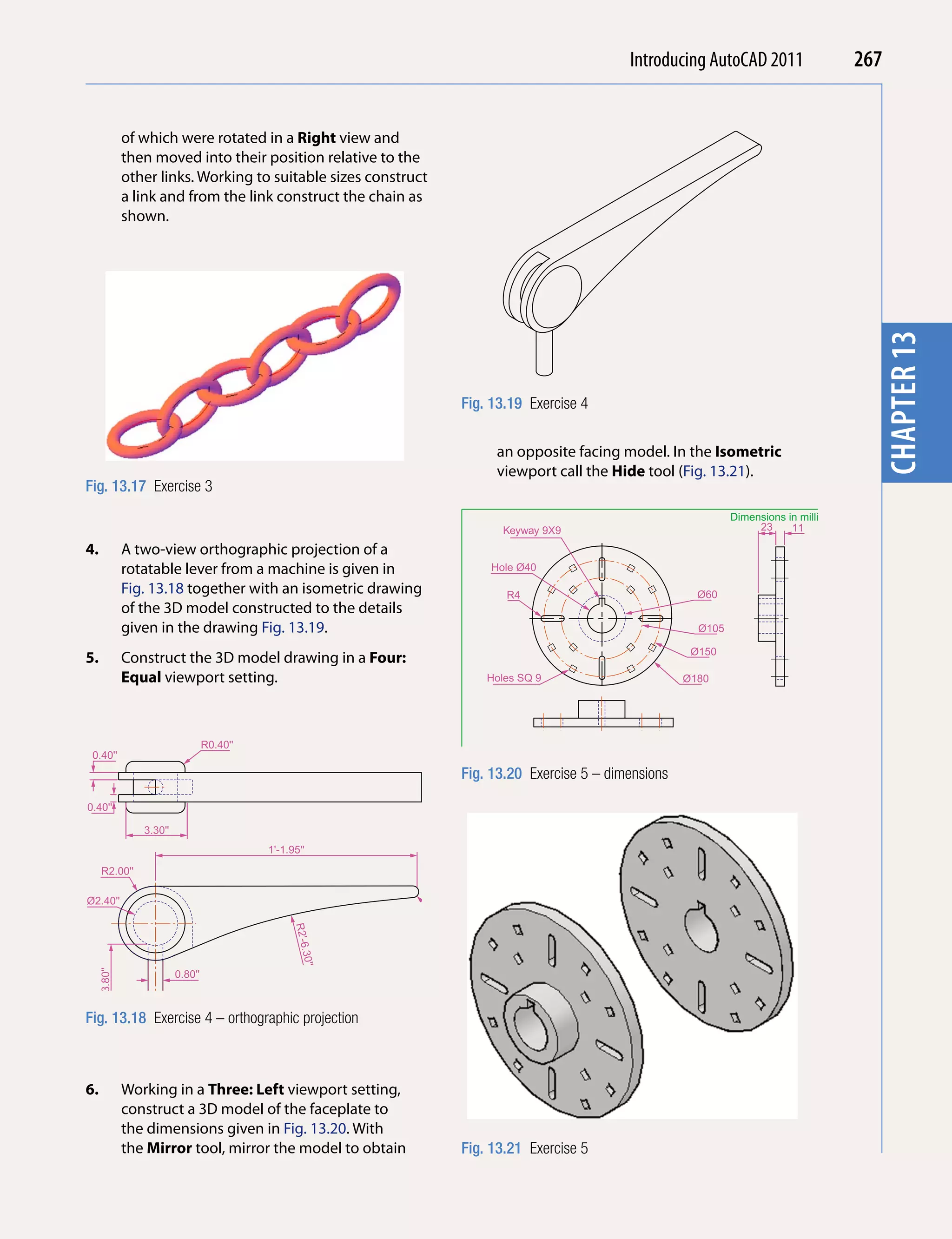
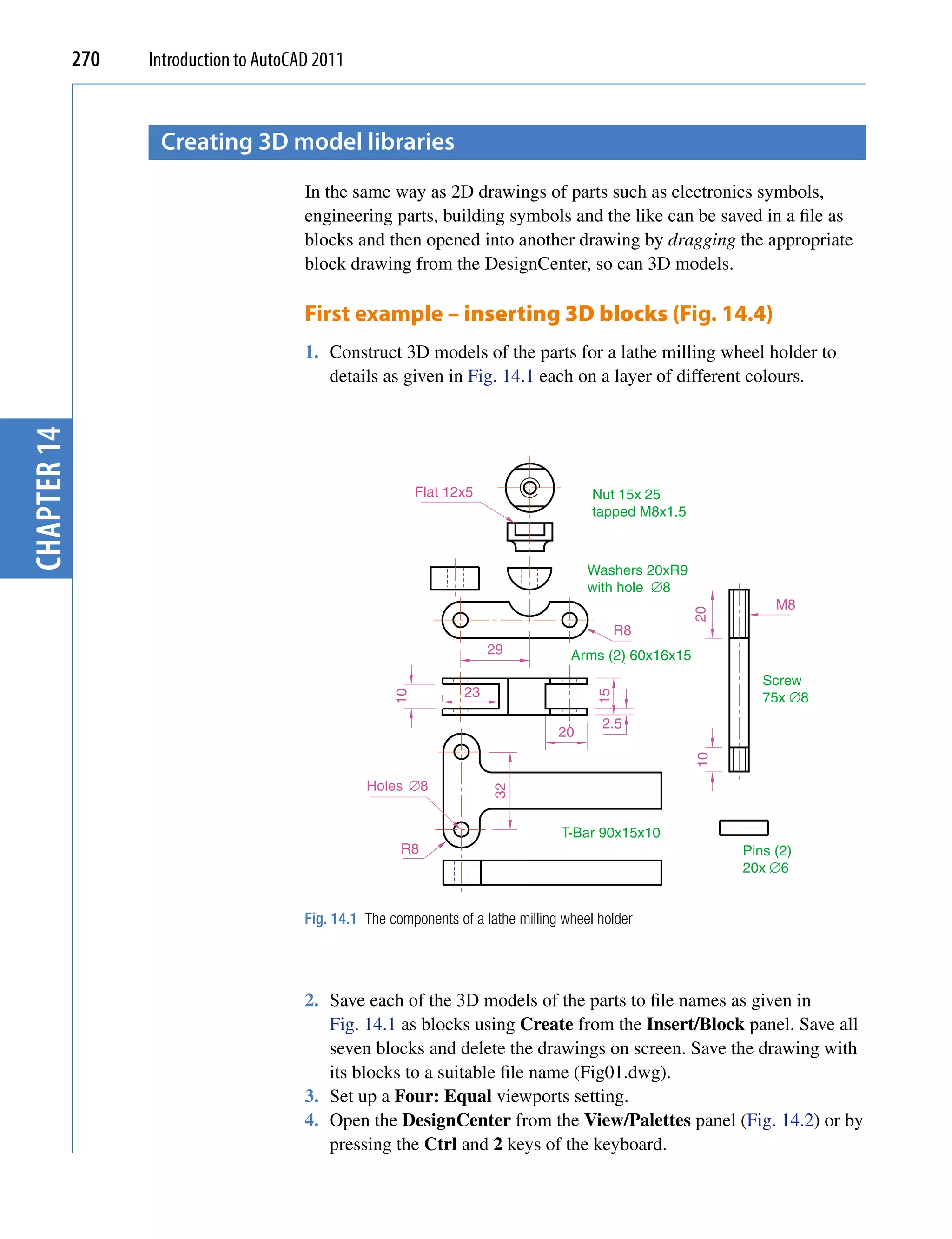
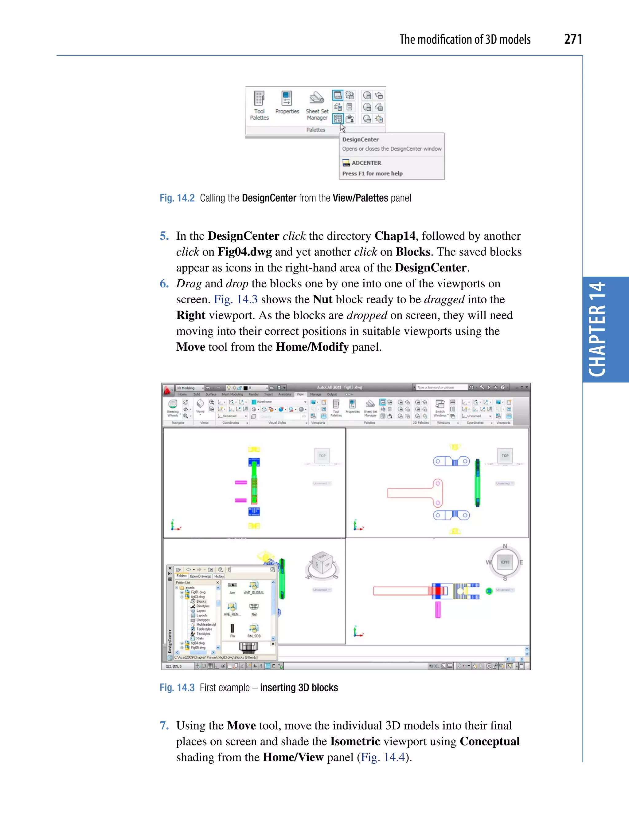
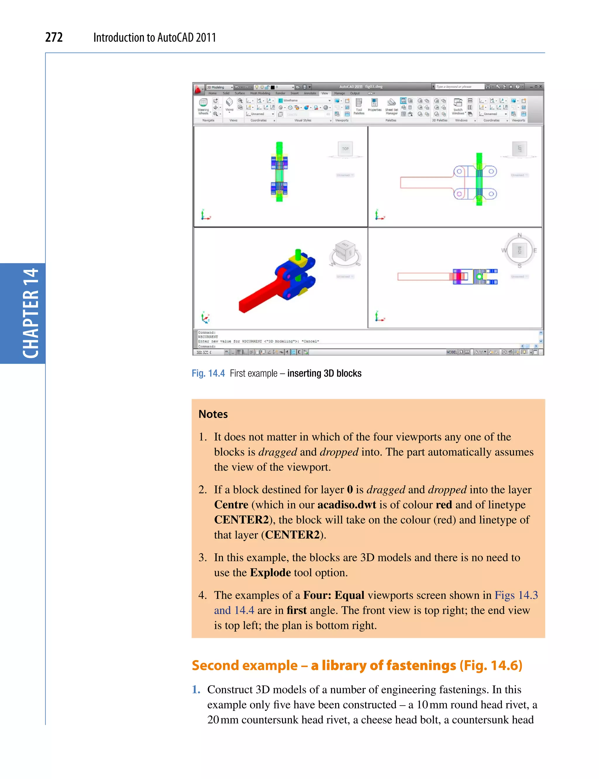
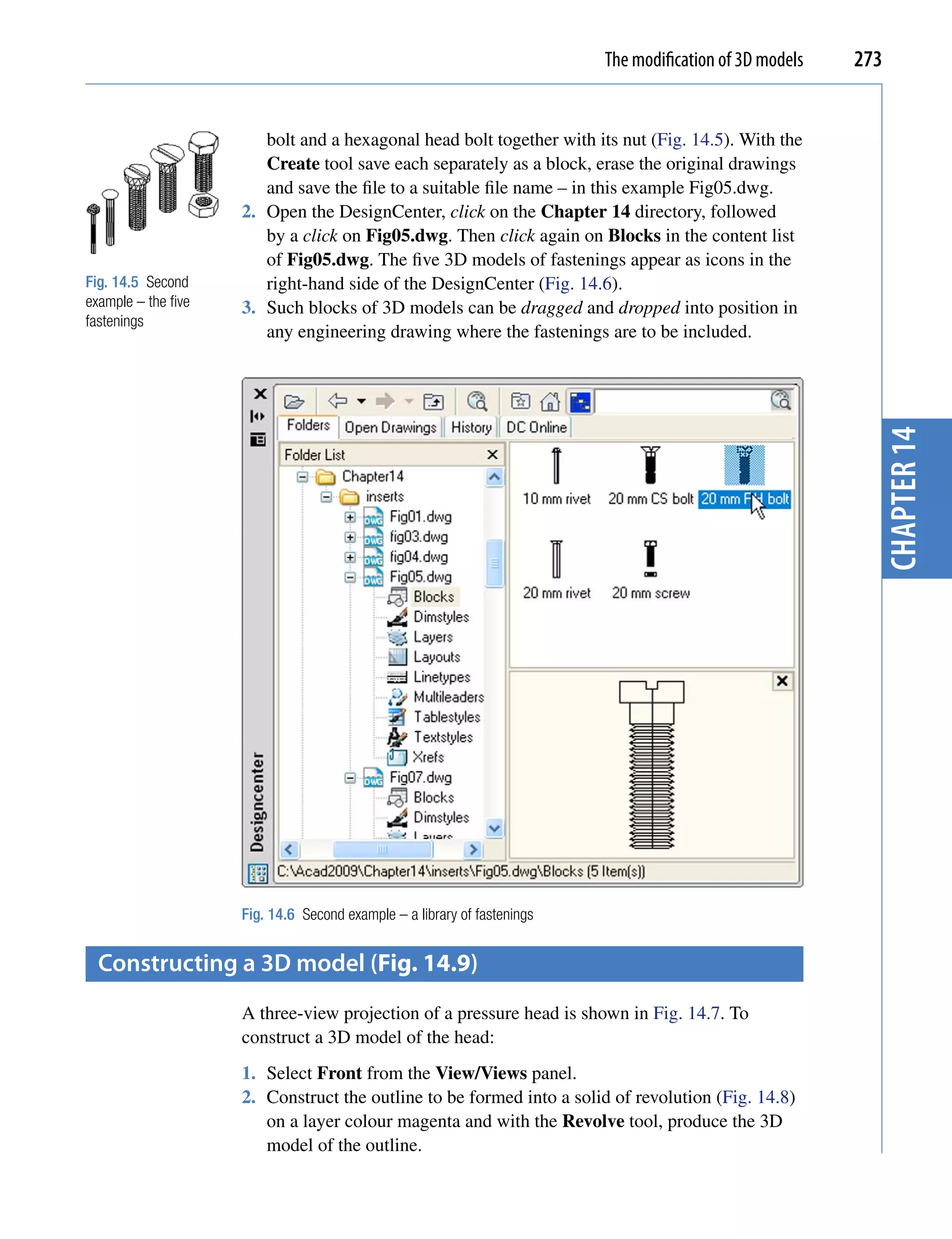
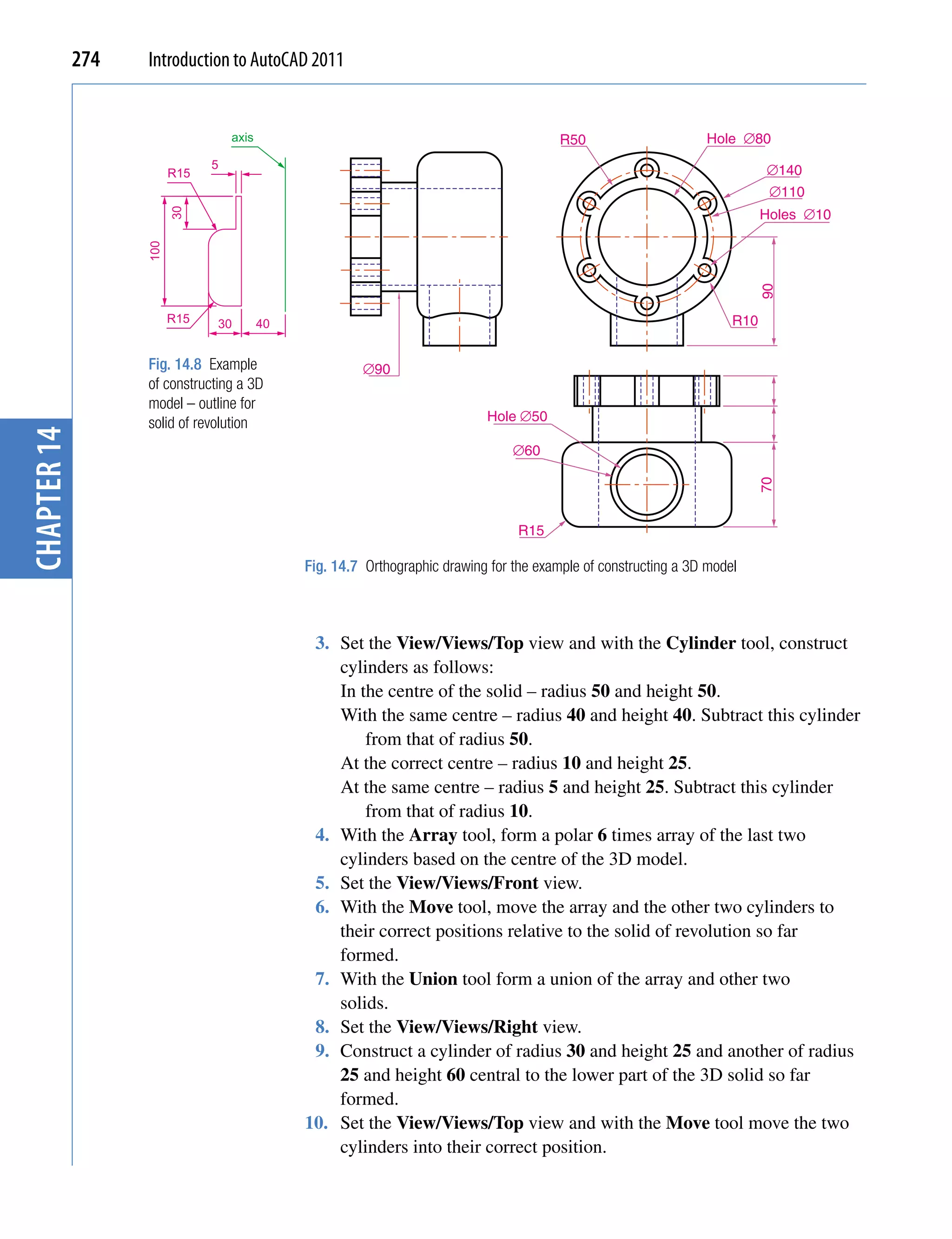
![The modification of 3D models 275
11. With Union, form a union between the radius 30 cylinder and the 3D
model and with Subtract, subtract the radius 25 cylinder from the 3D
model.
12. Click Realistic in the View/Visual Styles panel list.
The result is given in Fig. 14.9.
Fig. 14.9 Example Notes
of constructing a 3D
This 3D model could equally as well have been constructed in a three or
model
four viewports setting. Full Shading has been set on from the Render
ribbon, hence the line of shadows.
chapter 14
the 3D Array tool
First example – a Rectangular Array (Fig. 14.12)
1. Construct the star-shaped pline on a layer colour green (Fig. 14.10) and
extrude it to a height of 20.
2. Click on the 3D Array in the Home/Modify panel (Fig. 14.11). The
command line shows:
70
70
Fig. 14.10 Example –
3D Array – the star
pline
Fig. 14.11 Selecting 3D Array from the Home/Modify panel
Command:_3darray
Select objects: pick the extrusion 1 found
Select objects: right-click
Enter the type of array [Rectangular/Polar] <R>:
right-click
Enter the number of rows (---) <1>: enter 3 right-
click
Enter the number of columns (III): enter 3 right-
click
Enter the number of levels (...): enter 4 right-click](https://image.slidesharecdn.com/introductiontoautocad2011-100614022653-phpapp02/75/Introduction-to-AutoCad-2011-267-2048.jpg)
![276 Introduction to AutoCAD 2011
Specify the distance between rows (—): enter 100
right-click
Specify the distance between columns (III): enter
100 right-click
Specify the distance between levels (...): enter
300 right-click
Command:
3. Place the screen in the View/Views/SW Isometric view.
4. Shade using the View/Visual Styles/Shaded with Edges visual style
(Fig. 14.12).
Second example – a Polar Array (Fig. 14.13)
chapter 14
1. Use the same star-shaped 3D model.
2. Call the 3D Array tool again. The command line shows:
Fig. 14.12 First
example – a 3D Command:_3darray
Rectangular Array Select objects: pick the extrusion 1 found
Select objects: right-click
Enter the type of array [Rectangular/Polar] <R>:
enter p (Polar) right-click
Enter number of items in the array: 12
Specify the angle to fill (+=ccw), −=cw) <360>:
right-click
Rotate arrayed objects? [Yes/No] <Y>: right-click
Specify center point of array: 235,125
Specify second point on axis of rotation: 300,200
Command:
Fig. 14.13 Second example – a 3D Polar Array](https://image.slidesharecdn.com/introductiontoautocad2011-100614022653-phpapp02/75/Introduction-to-AutoCad-2011-268-2048.jpg)
![The modification of 3D models 277
3. Place the screen in the View/Views/SW Isometric view.
4. Shade using the View/Visual Styles Shaded visual style (Fig. 14.13).
Third example – a Polar Array (Fig. 14.15)
Ø10 Ø20
1. Working on a layer of colour red, construct a solid of revolution in the
50 30 form of an arrow to the dimensions as shown in Fig. 14.14.
2. Click 3D Array in the Home/Modify panel. The command line
Fig. 14.14 Third
shows:
example – a 3D Polar
Array – the 3D model Command: _3darray
to be arrayed
Select objects: pick the arrow 1 found
Select objects: right-click
chapter 14
Enter the type of array [Rectangular/Polar]<R>:
enter p right-click
Enter the number of items in the array: enter 12
right-click
Specify the angle to fill (+=ccw, −=cw) <360>:
right-click
Rotate arrayed objects? [Yes/No] <Y>:
right-click
Specify center point of array: enter 40,170,20
right-click
Specify second point on axis of rotation: enter
60,200,100 right-click
Command:
3. Place the array in the 3D Navigate/SW Isometric view and shade
to View/Visual Styles/Shades of Gray. The result is shown in
Fig. 14.15.
Fig. 14.15 Third example – a 3D Polar Array](https://image.slidesharecdn.com/introductiontoautocad2011-100614022653-phpapp02/75/Introduction-to-AutoCad-2011-269-2048.jpg)
![278 Introduction to AutoCAD 2011
the 3D mirror tool
First example – 3D Mirror (Fig. 14.17)
15 1. Working on a layer colour green, construct the outline Fig. 14.16.
10
First point
Third point 2. Extrude the outline to a height of 20.
50
25
3. Extrude the region to a height of 5 and render. A Conceptual style
shading is shown in Fig. 14.17 (left-hand drawing).
20
140
30
chapter 14
180
Second point
Fig. 14.16 First
example – 3D Mirror –
outline of object to be
mirrored
Fig. 14.17 First example – 3D Mirror – before and after Mirror
4. Click on 3D Mirror in the 3D Operation sub-menu of the Modify
drop-down menu. The command line shows:
Command:_3dmirror
Select objects: pick the extrusion 1 found
Select objects: right-click
Specify first point of mirror plane (3 points): pick
Specify second point on mirror plane: pick
Specify third point on mirror plane or [Object/
Last/Zaxis/View/XY/YZ/ZX/3points]: enter .xy
right-click of (need Z): enter 1 right-click
Delete source objects? [Yes/No]: <N>: right-click
Command:
The result is shown in the right-hand illustration of Fig. 14.17.](https://image.slidesharecdn.com/introductiontoautocad2011-100614022653-phpapp02/75/Introduction-to-AutoCad-2011-270-2048.jpg)
![The modification of 3D models 279
Second example – 3D Mirror (Fig. 14.19)
1. Construct a solid of revolution in the shape of a bowl in the 3D Navigate/
Front view working on a layer of colour magenta (Fig. 14.18).
Fig. 14.18 Second example – 3D Mirror – the 3D model
2. Click 3D Mirror in the Home/Modify panel. The command line
shows:
chapter 14
Command:_3dmirror
Select objects: pick the bowl 1 found
Select objects: right-click
Specify first point on mirror plane (3 points):
pick
Specify second point on mirror plane: pick
Specify third point on mirror plane: enter .xy
right-click (need Z): enter 1 right-click
Delete source objects:? [Yes/No]: <N>: right-click
Command:
The result is shown in Fig. 14.19.
3. Place in the 3D Navigate/SW Isometric view.
4. Shade using the View/Visual Styles Conceptual visual style (Fig. 14.19).
Fig. 14.19 Second example – 3D Mirror – the result in a front view](https://image.slidesharecdn.com/introductiontoautocad2011-100614022653-phpapp02/75/Introduction-to-AutoCad-2011-271-2048.jpg)
![280 Introduction to AutoCAD 2011
the 3D rotate tool
Example – 3D Rotate (Fig. 14.20)
1. Use the same 3D model of a bowl as for the last example. Pick 3D
Rotate tool from the Home/Modify panel. The command line shows:
Command:_3drotate
Current positive angle in UCS:
ANGDIR=counterclockwise ANGBASE=0
Select objects: pick the bowl 1 found
Select objects: right-click
Specify base point: pick the centre bottom of the
bowl
chapter 14
Specify rotation angle or [Copy/Reference] <0>:
enter 60 right-click
Command
Fig. 14.20 Example – 2. Place in the 3D Navigate/SW Isometric view and in Conceptual
3D Rotate shading.
The result is shown in Fig. 14.20.
the slice tool
First example – Slice (Fig. 14.24)
1. Construct a 3D model of the rod link device shown in the two-view
projection (Fig. 14.21) on a layer colour green.
5 Hole Ø30
R20
Hole Ø40 Ø60
20
60
5
220
Fig. 14.21 First example – Slice – the two-view drawing](https://image.slidesharecdn.com/introductiontoautocad2011-100614022653-phpapp02/75/Introduction-to-AutoCad-2011-272-2048.jpg)
![The modification of 3D models 281
2. Place the 3D model in the 3D Navigation/Top view.
3. Call the Slice tool from the Home/Solid Editing panel (Fig. 14.22).
chapter 14
Fig. 14.22 The Slice tool icon from the Home/Solid Editing panel
The command line shows:
Command:_slice
Select objects: pick the 3D model
Select objects to slice: right-click
Specify start point of slicing plane or [planar
Object/Surface/Zaxis/View/XY/YZ/ZX/3points]
<3points>: pick
Specify second point on plane: pick
Specify a point on desired side or [keep Both
sides] <Both>: right-click
Command:
Fig. 14.23 shows the picked points.
start point second point
Fig. 14.23 First example – Slice – the pick points
4. With the Move tool, move the lower half of the sliced model away from
the upper half.
Fig. 14.24 First 5. Place the 3D model(s) in the ViewCube/Isometric view.
example – Slice 6. Shade in Conceptual visual style. The result is shown in Fig. 14.24.](https://image.slidesharecdn.com/introductiontoautocad2011-100614022653-phpapp02/75/Introduction-to-AutoCad-2011-273-2048.jpg)
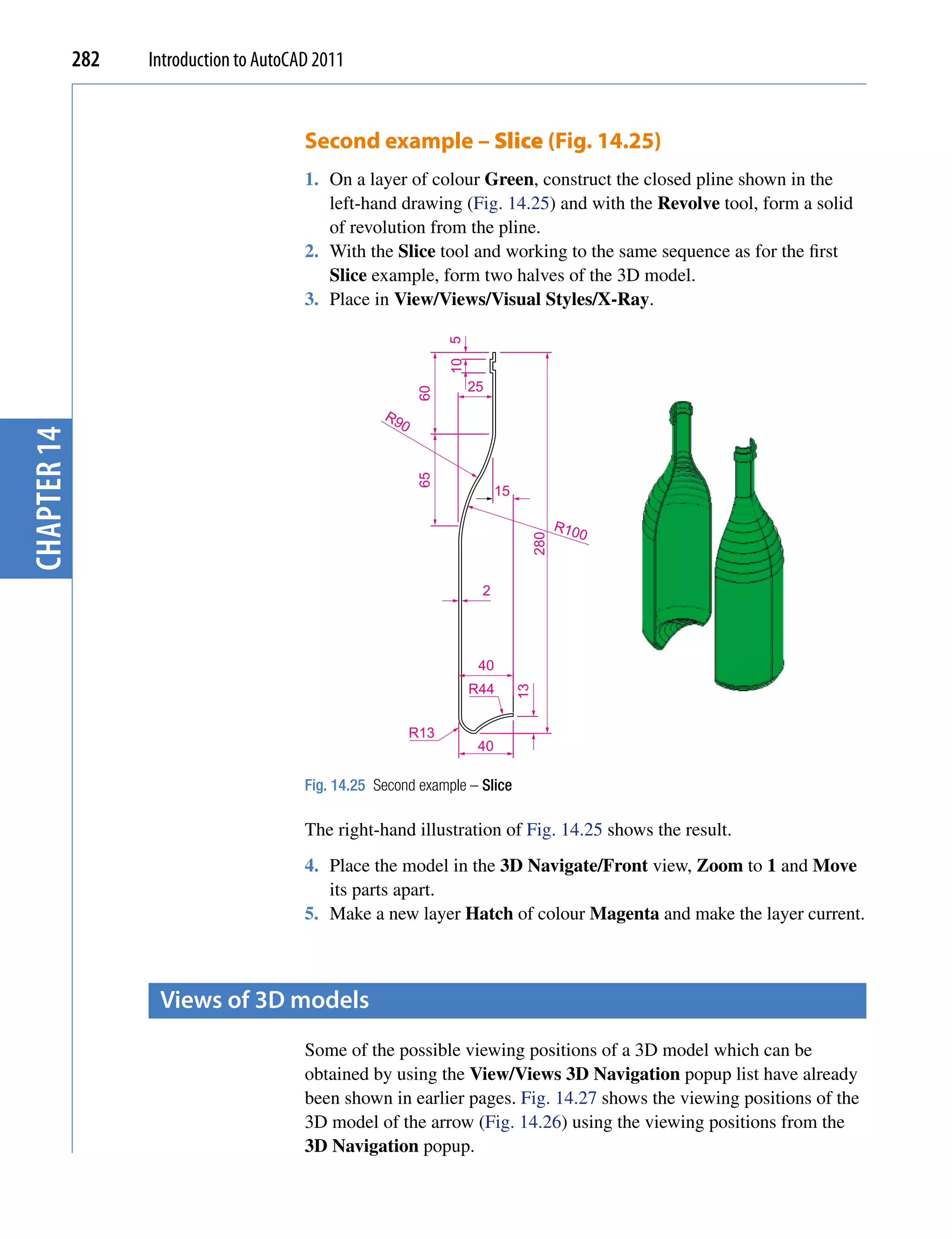
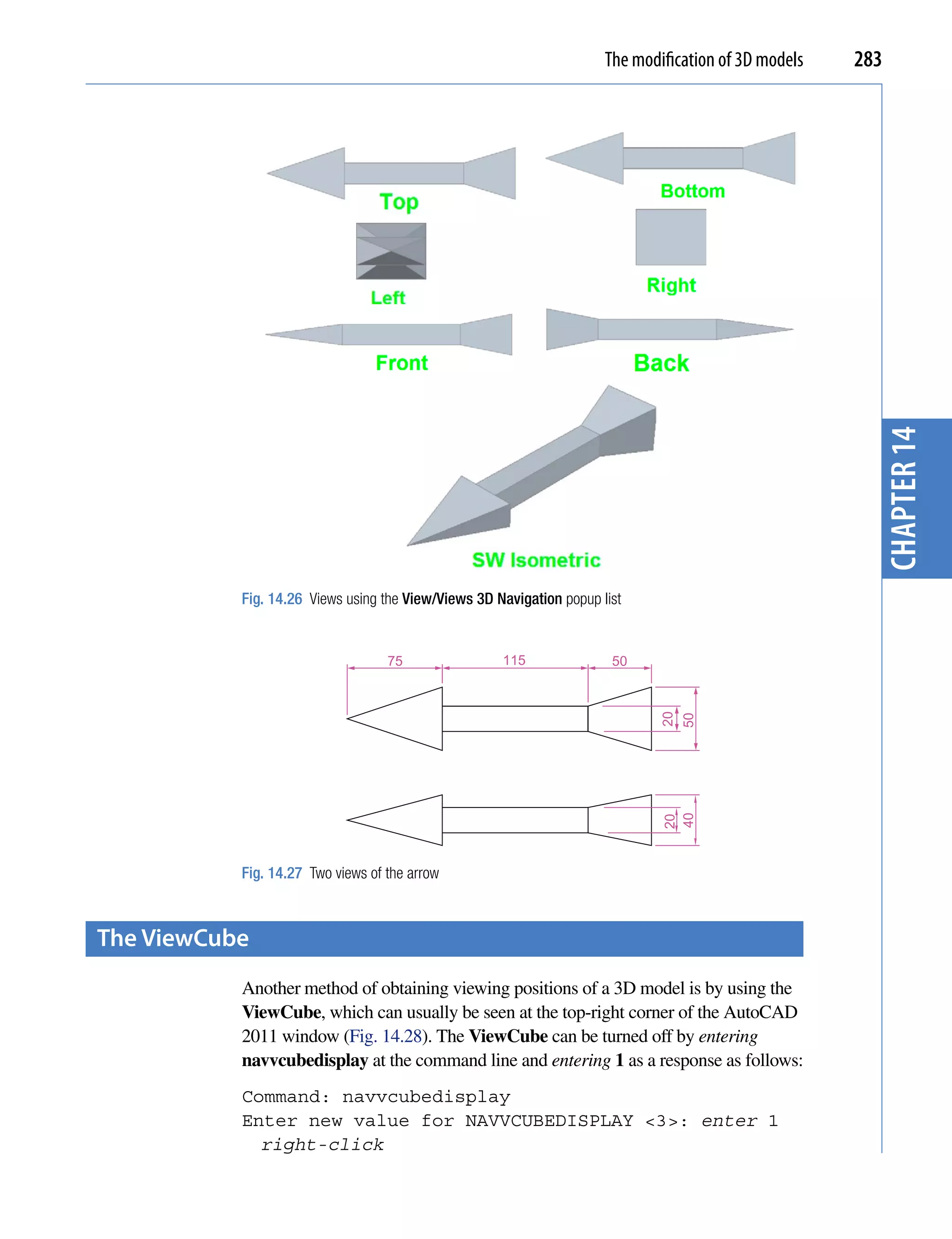
![chapter 14 284 Introduction to AutoCAD 2011
Fig. 14.28 The ViewCube
Entering 3 as a response to navvcubedisplay causes the ViewCube to
reappear.
The ViewCube is used as follows:
Click on Top and the Top view of a 3D model appears.
Click on Front and the Front view of a 3D model appears.
And so on. Clicking the arrows at top, bottom or sides of the ViewCube
moves a model between views.
A click on the house icon at the top of the ViewCube places a model in the
SW Isometric view.
Using Dynamic input to construct a helix
As with all other tools (commands) in AutoCAD 2011 a helix can be
formed working with the Dynamic Input (DYN) system. Fig. 14.30 shows
the stages (1 to 5) in the construction of the helix in the second example.
Set DYN on with a click on its button in the status bar.
1. Click the Helix tool icon in the Home/Draw panel (Fig. 14.29). The
first of the DYN prompts appears. Enter the following at the command
line using the down key of the keyboard when necessary.
Command: _Helix
Number of turns=10 Twist=CCW
Specify center point of base: enter 95,210
Specify base radius or [Diameter]: enter 55](https://image.slidesharecdn.com/introductiontoautocad2011-100614022653-phpapp02/75/Introduction-to-AutoCad-2011-276-2048.jpg)
![The modification of 3D models 285
chapter 14
Fig. 14.29 The Helix tool in the Home/Draw panel
Specify top radius or [Diameter]: enter 35
Specify helix height or [Axis endpoint/Turns/turn
Height/tWist]: enter 100
Command:
Fig. 14.30 shows the sequence of DYN tooltips and the completed helix.
Fig. 14.30 Constructing the helix for the second example with the aid of DYN](https://image.slidesharecdn.com/introductiontoautocad2011-100614022653-phpapp02/75/Introduction-to-AutoCad-2011-277-2048.jpg)
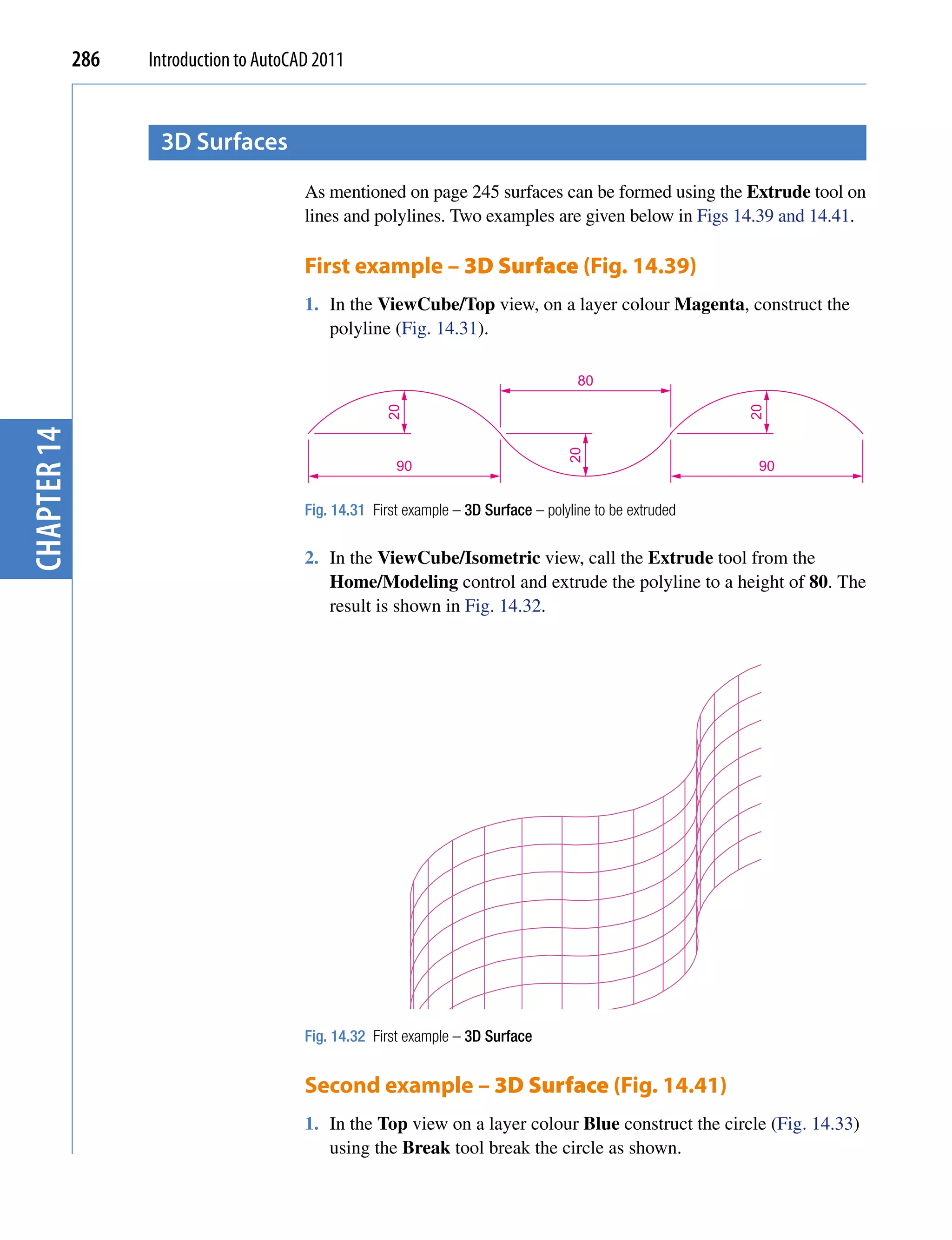
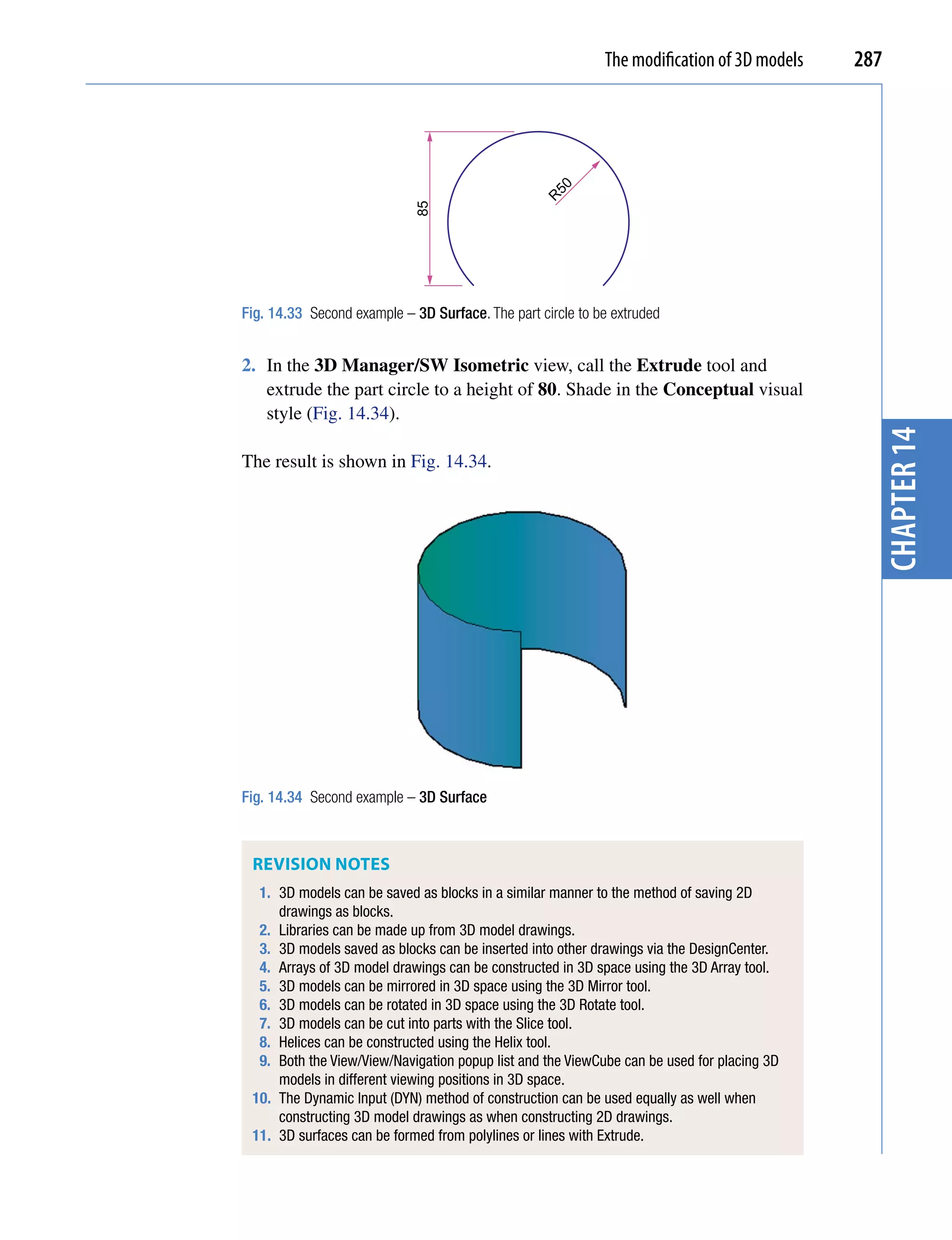
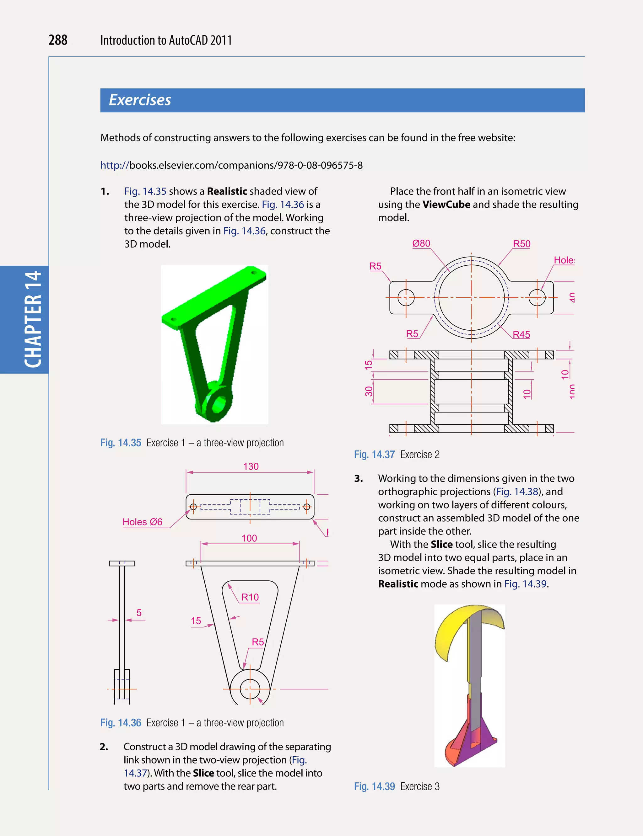
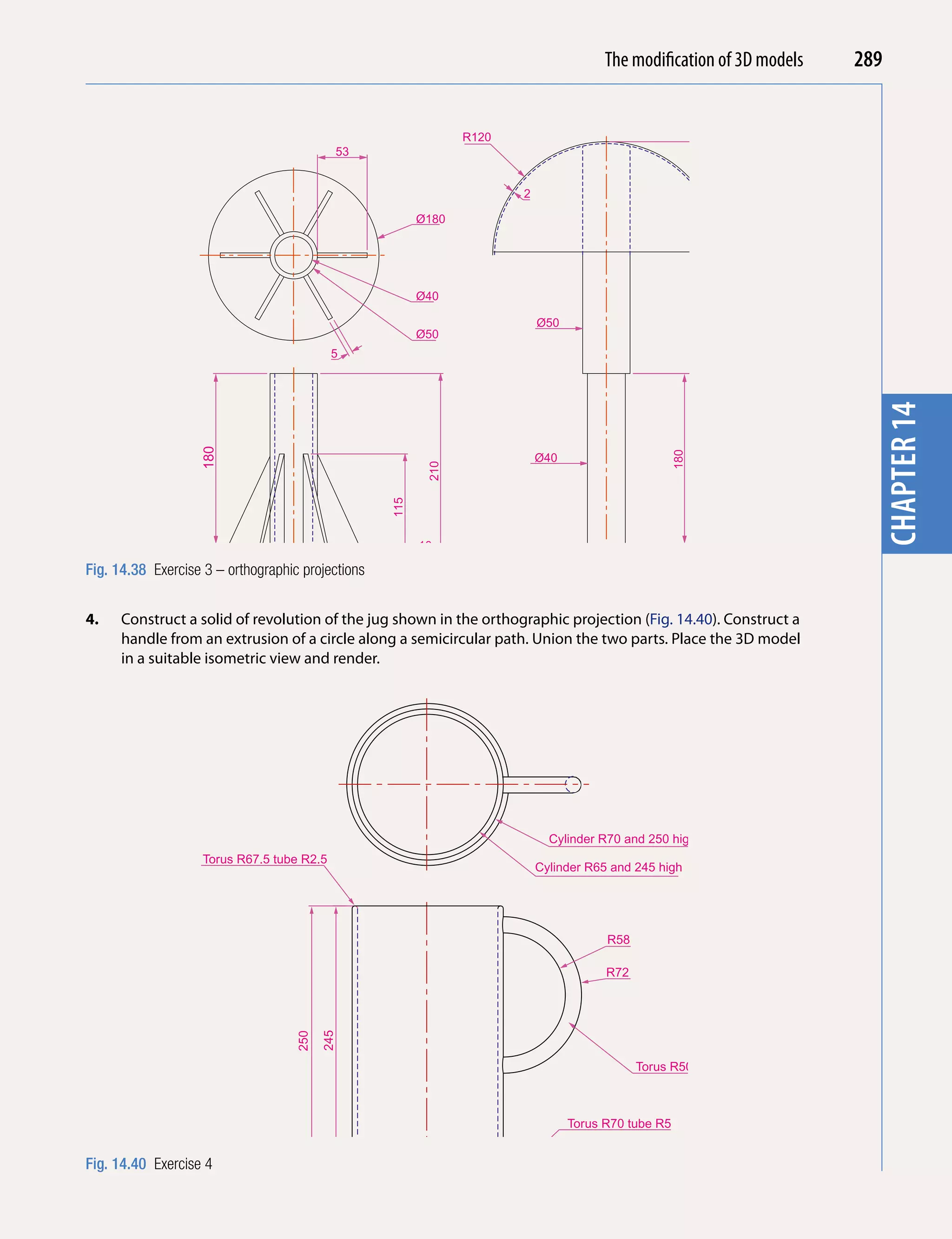
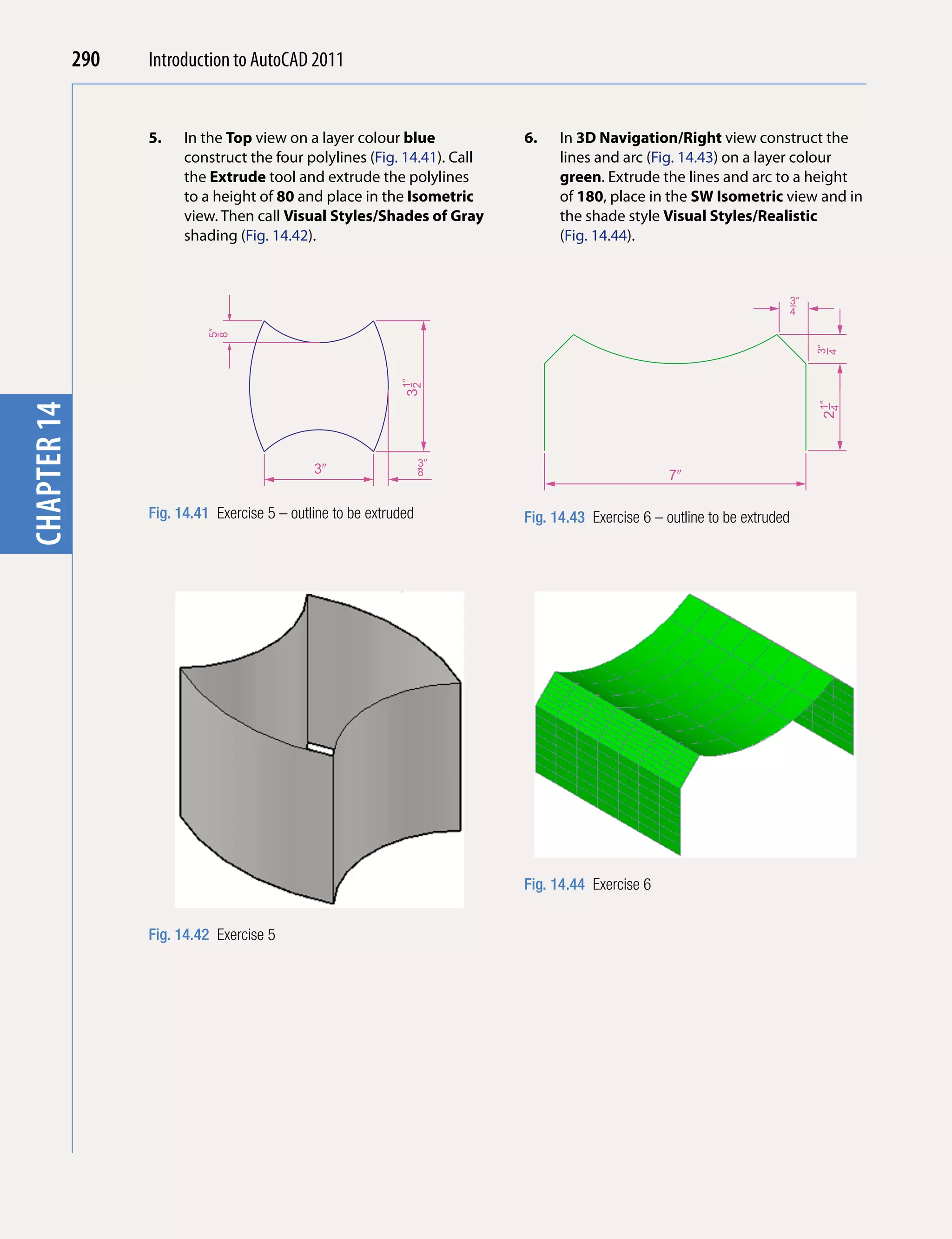
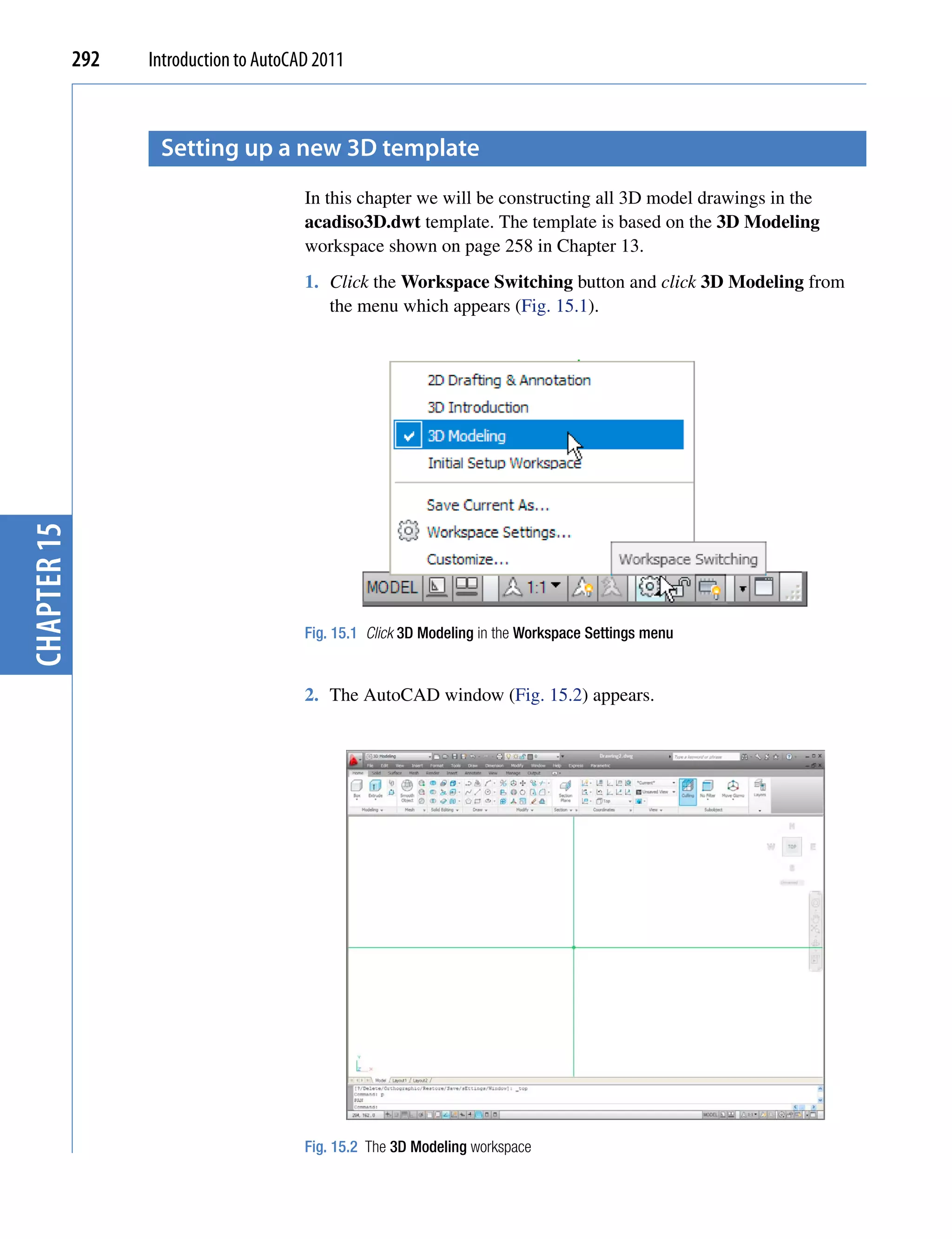
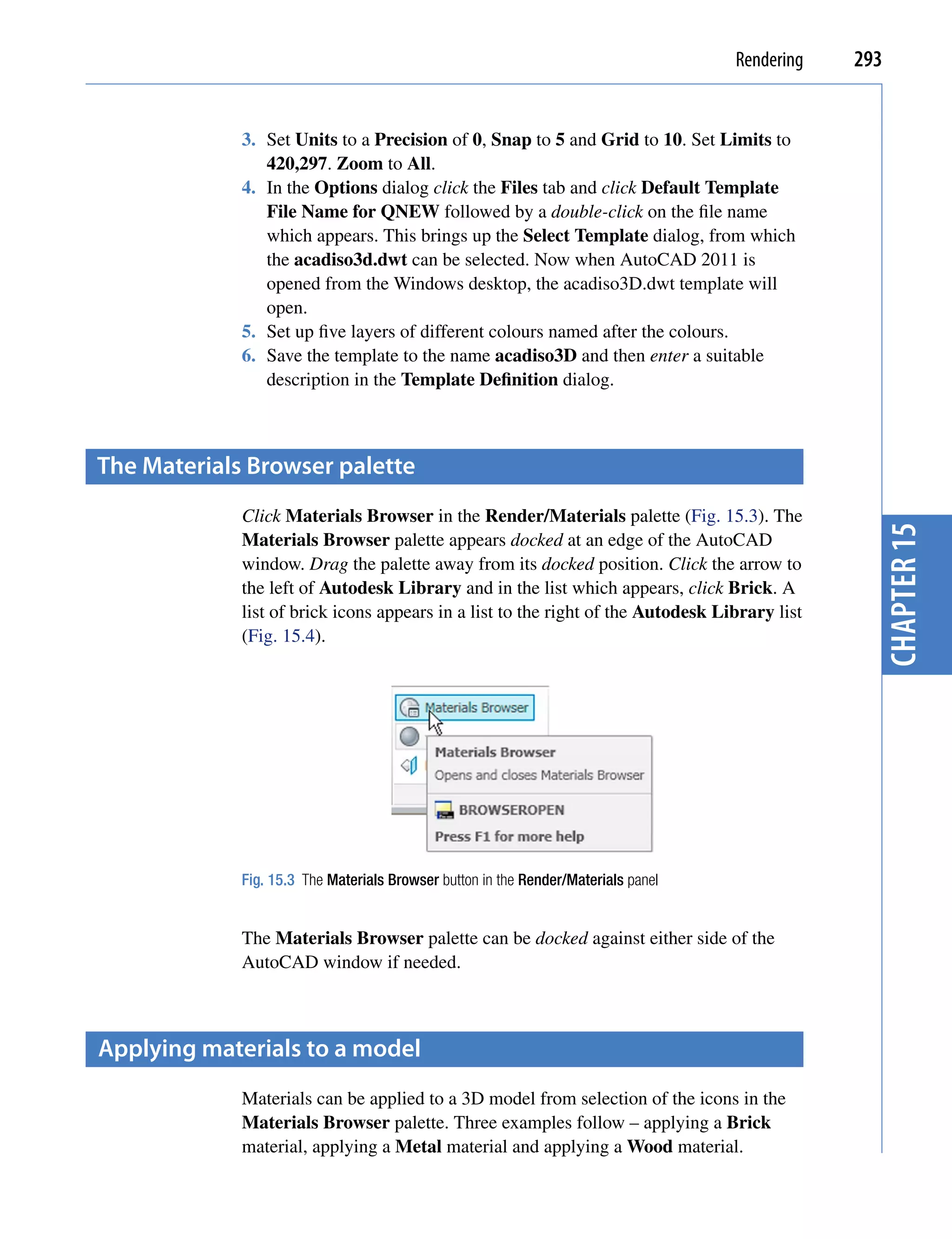
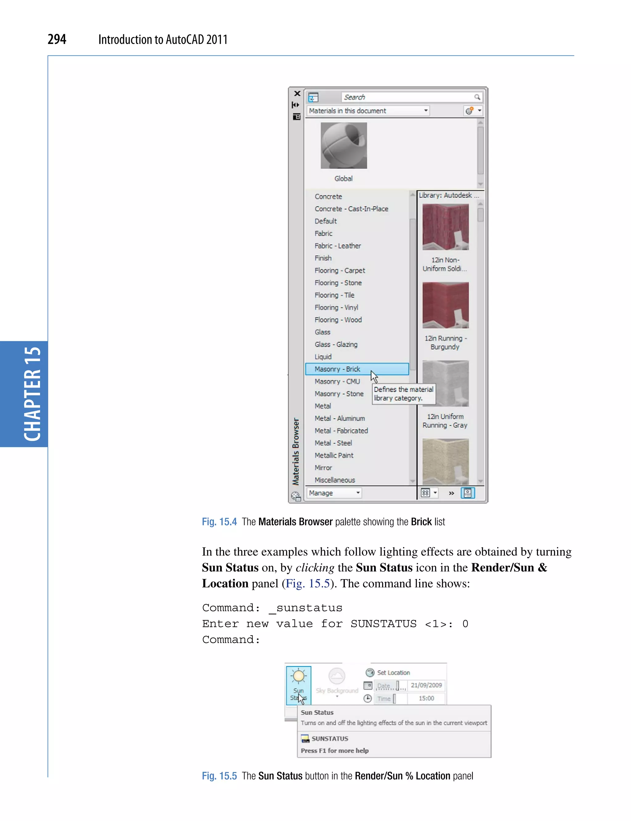
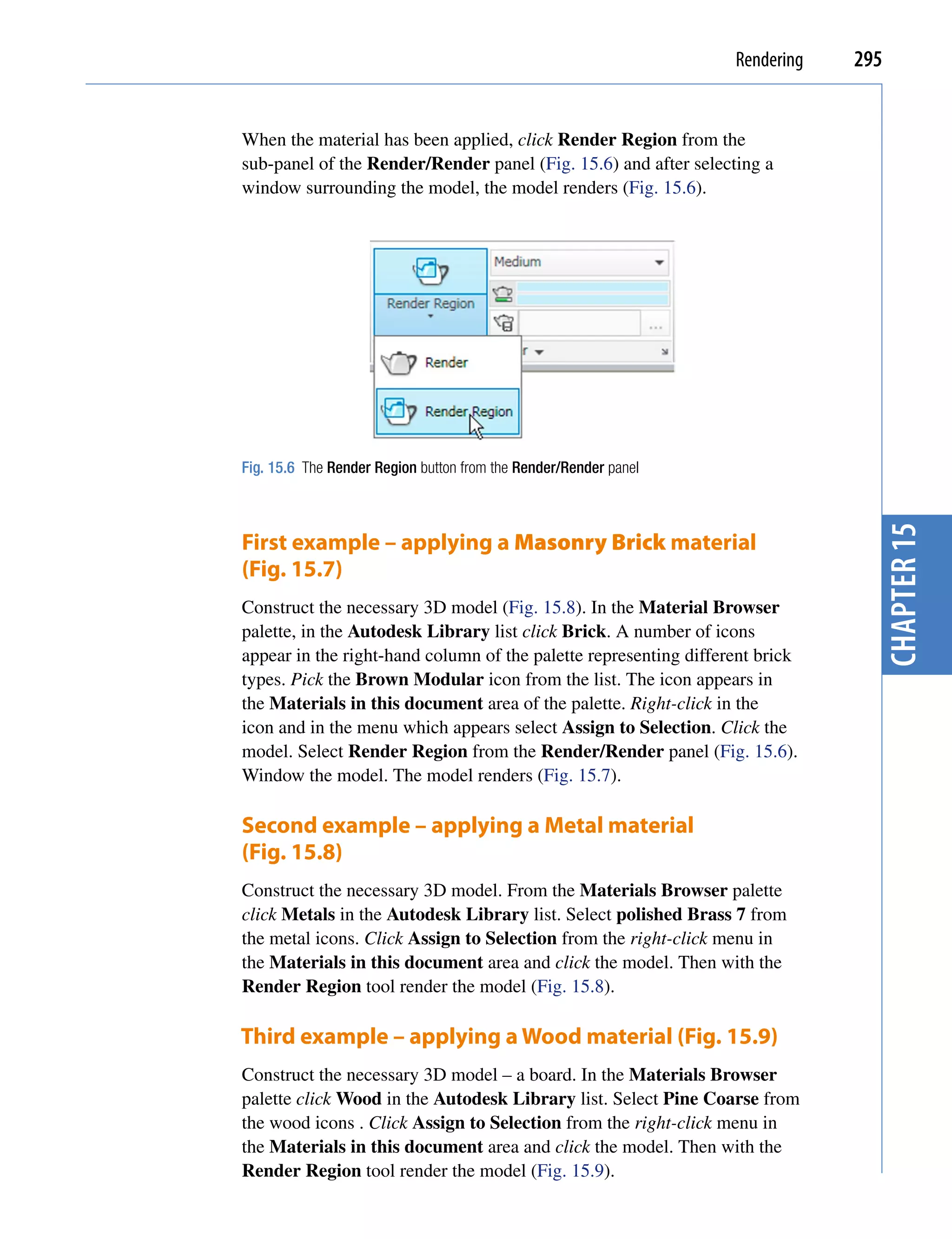
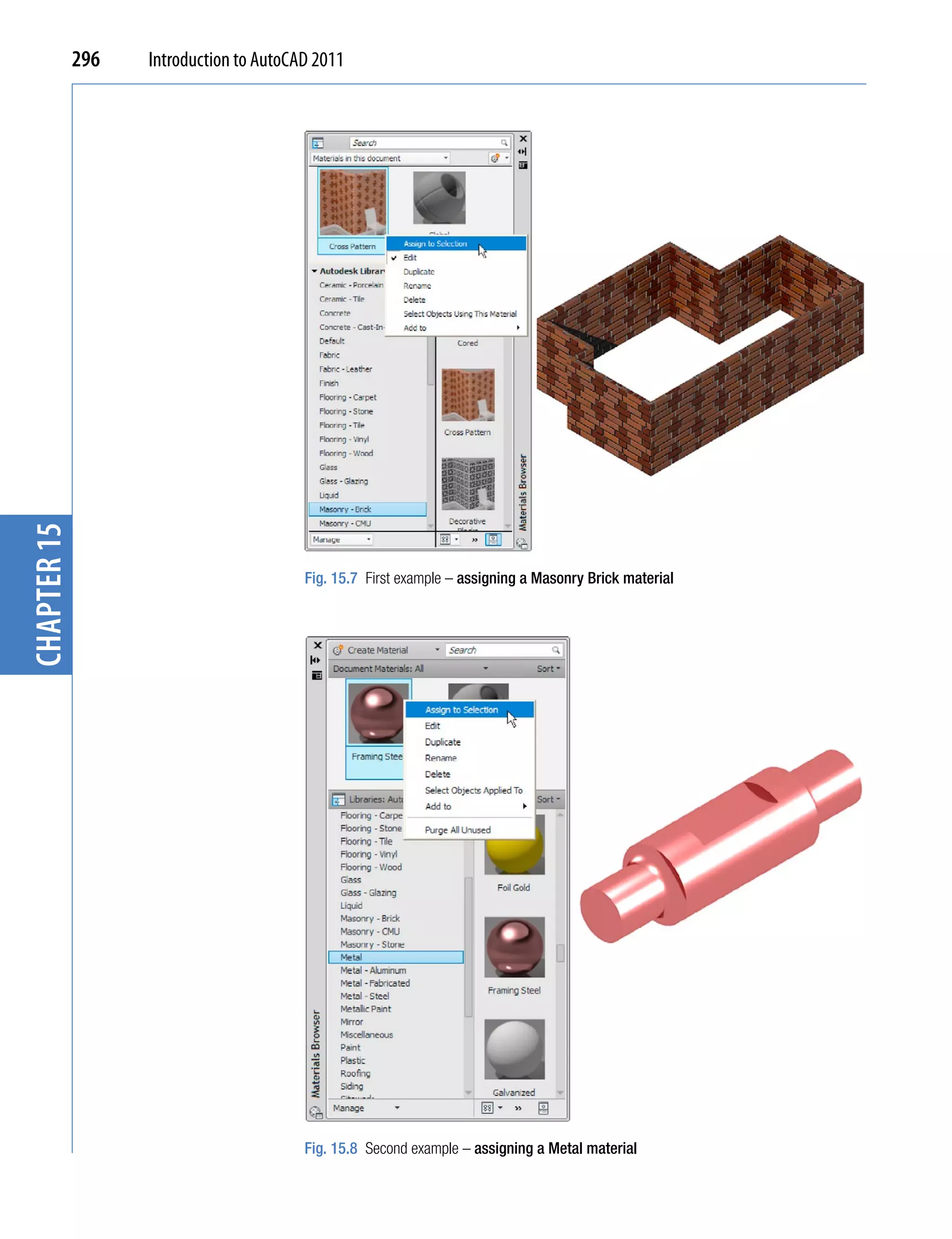
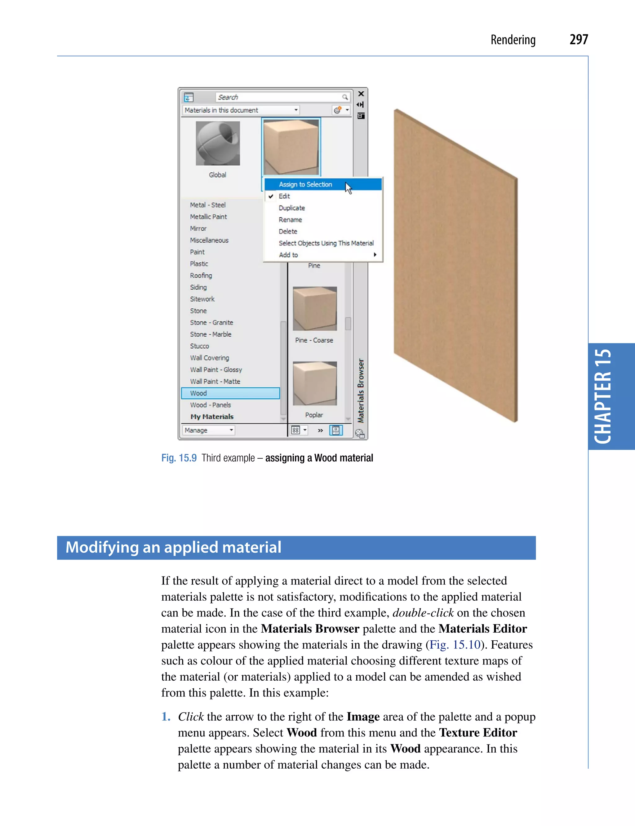
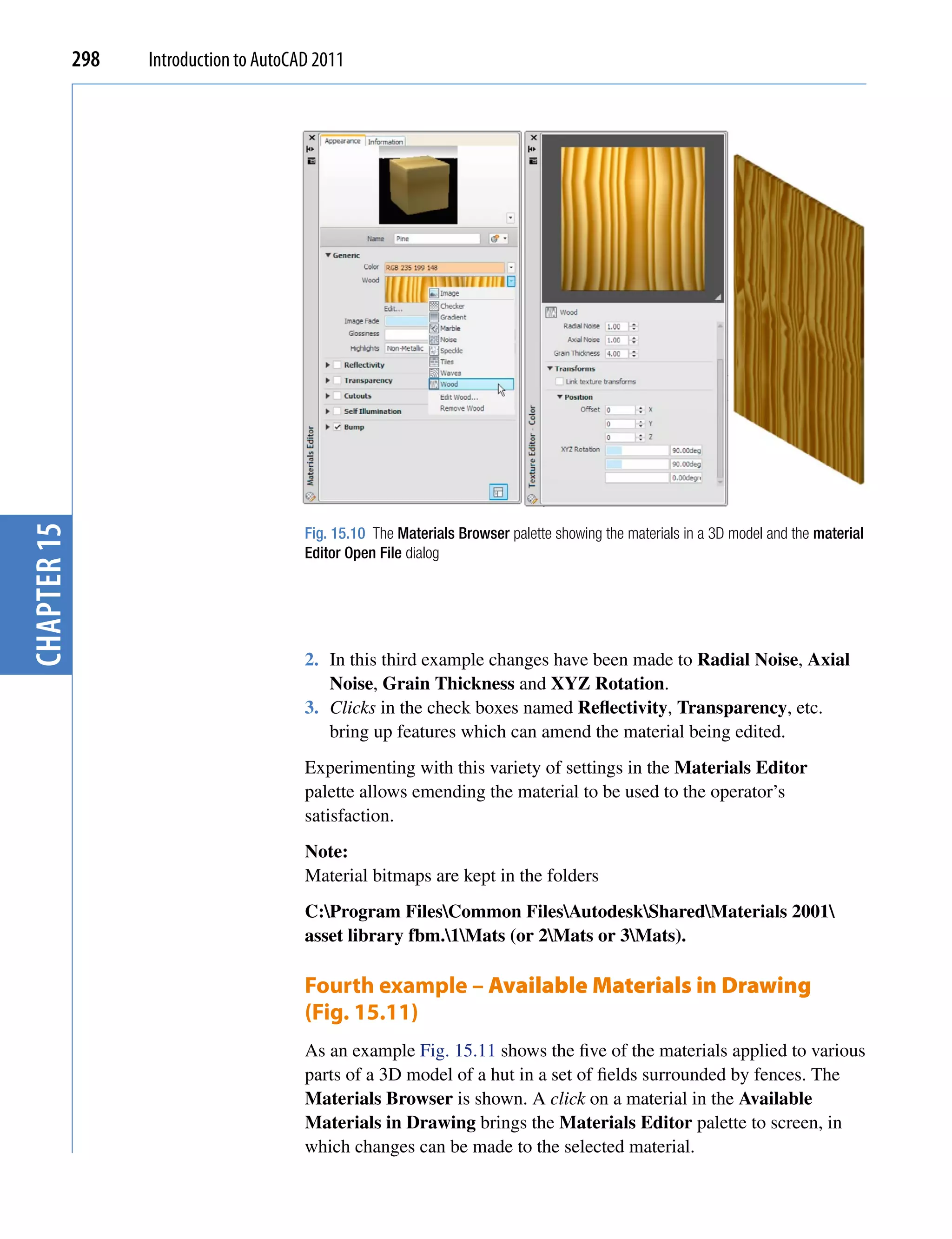
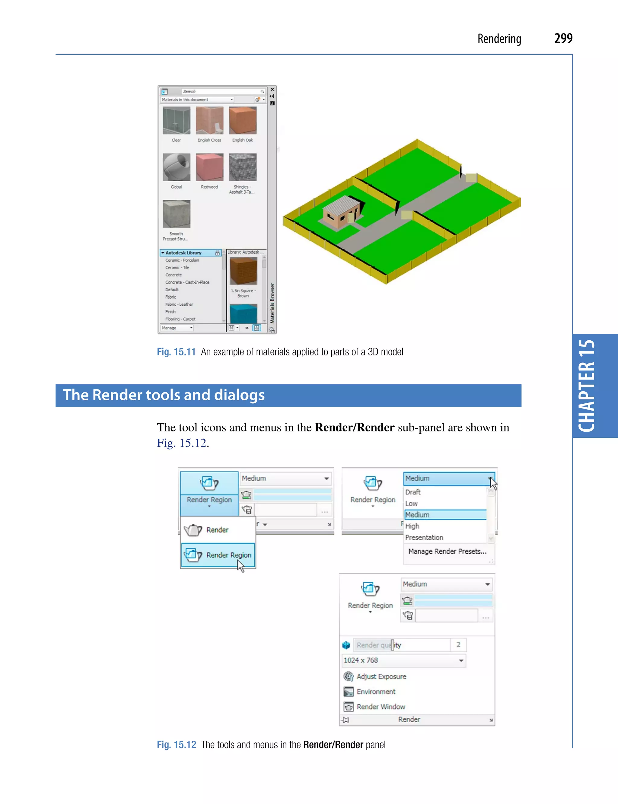
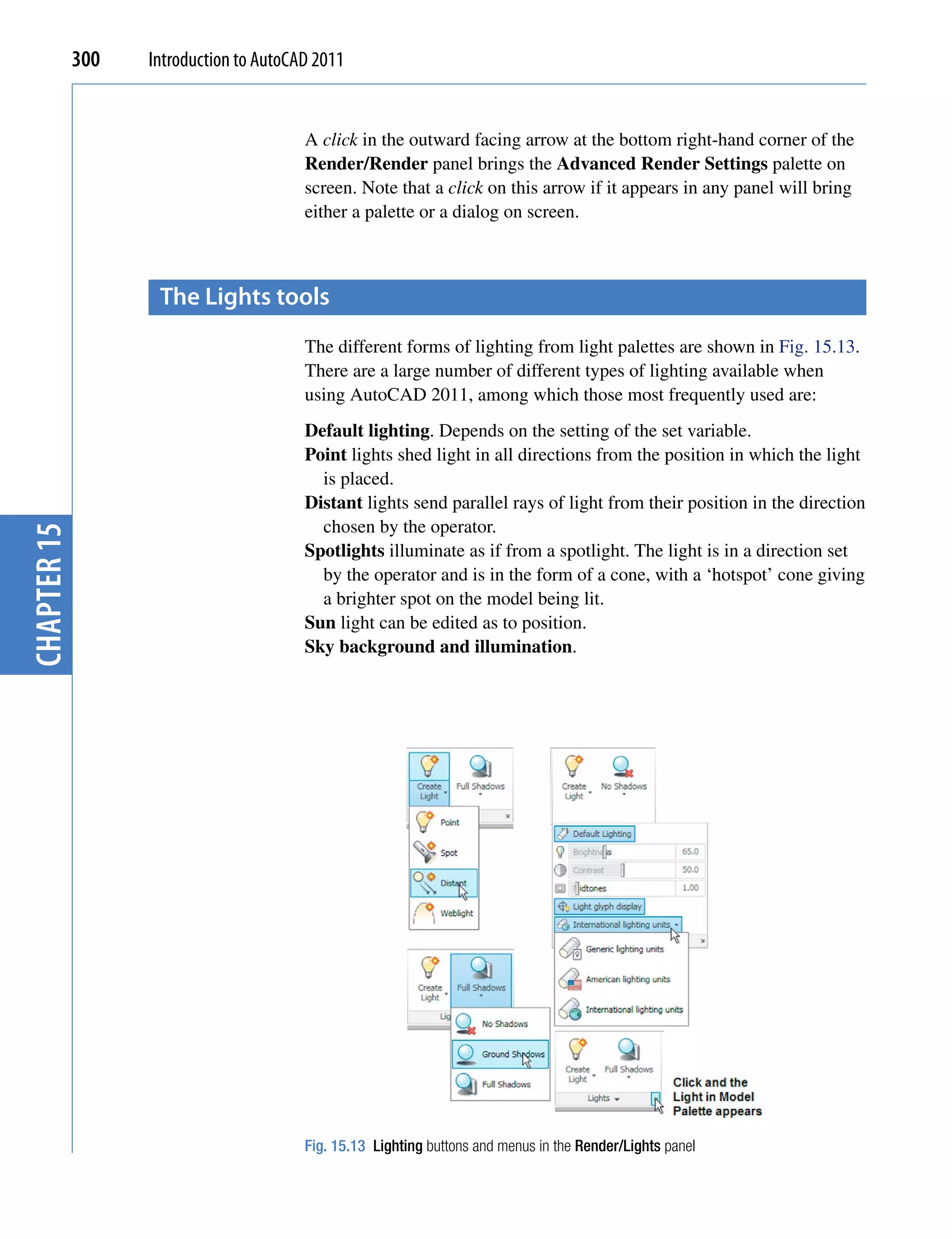
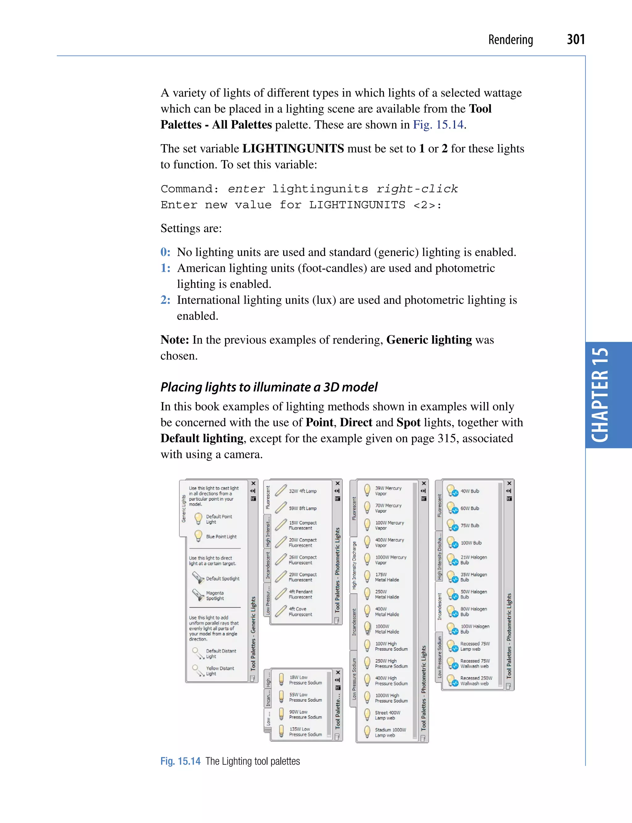
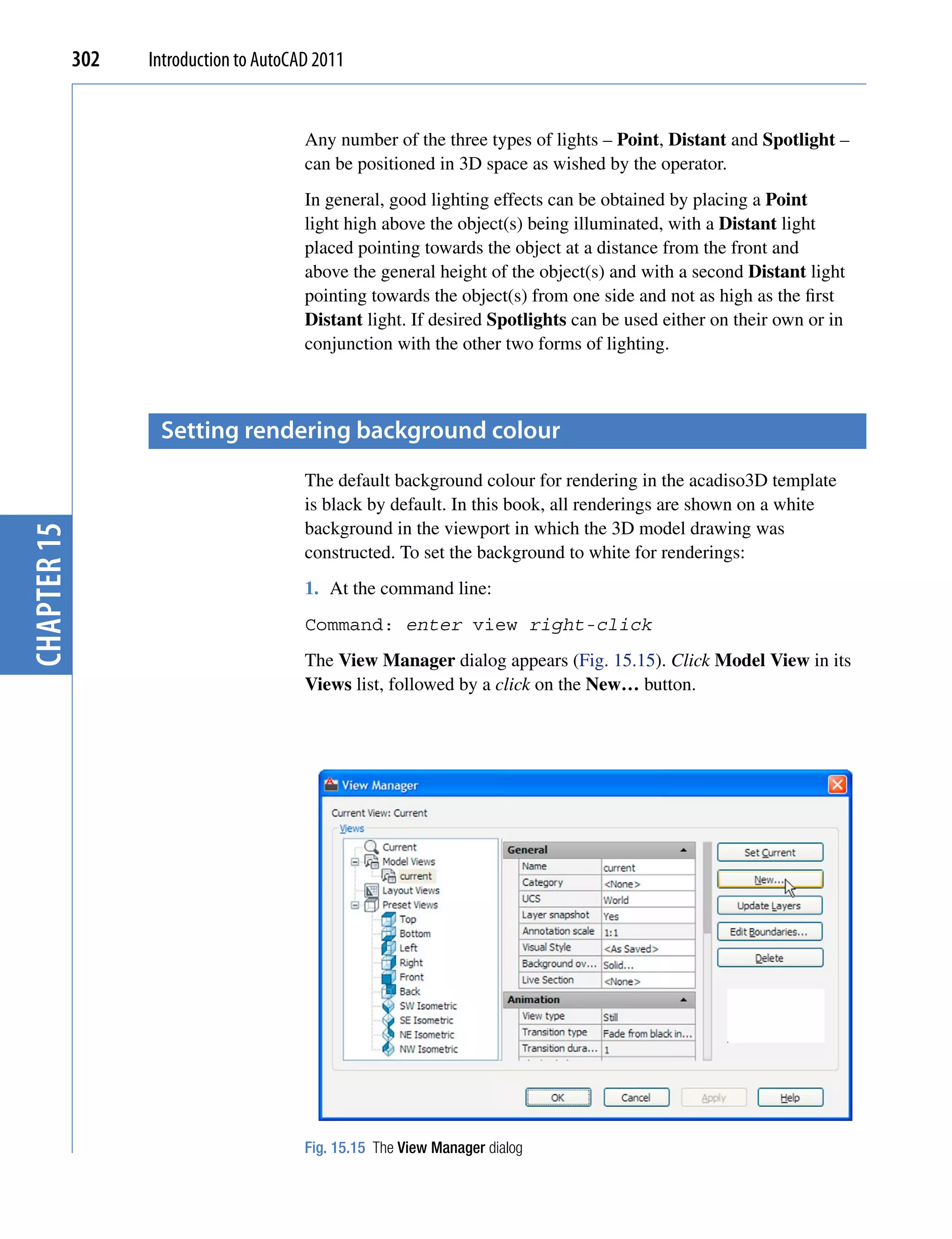
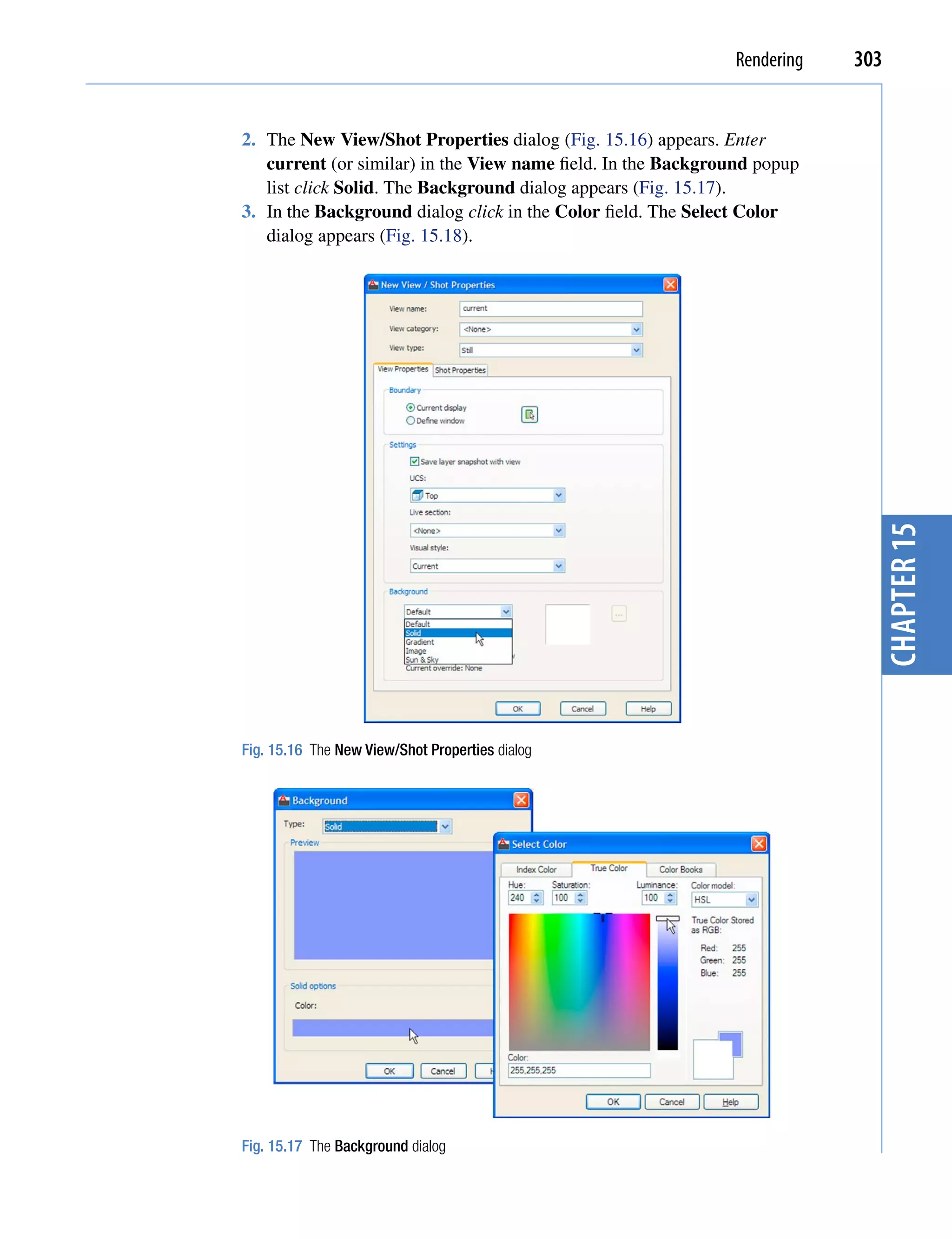
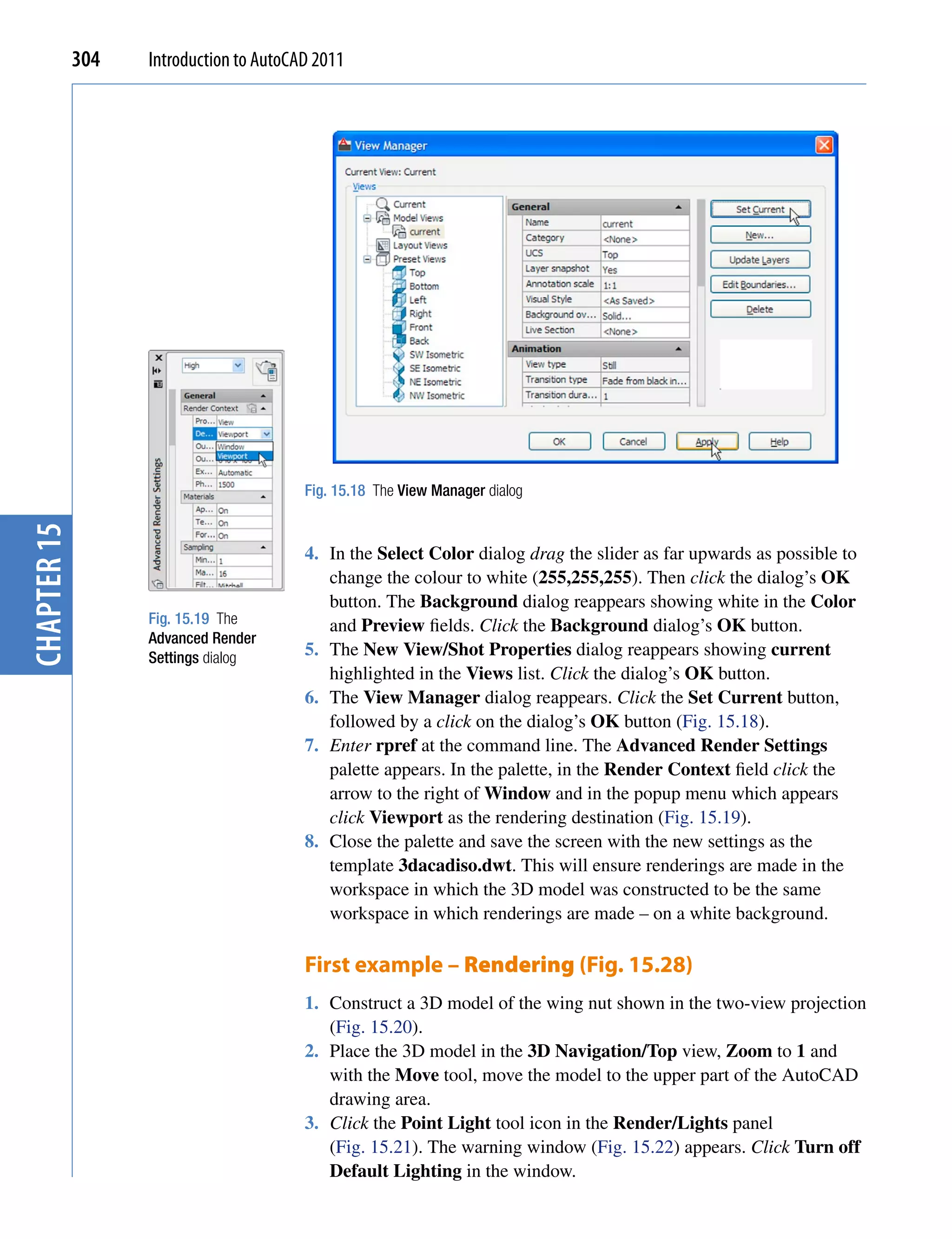
![Rendering 305
Ø60
10
Tapped M45
95
35 65 R10
20
R2
140
60
20
R10
115
Fig. 15.21 The Point Light icon in the
Fig. 15.20 First example – Rendering – Render/Lights panel
two-view projection
chapter 15
Fig. 15.22 The Lighting – Viewport Lighting Mode warning window
4. A New Point Light icon appears (depending upon the setting of the
Light Glyph Setting in the Drafting area of the Options dialog) and
the command line shows:
Command:_pointlight
Specify source location <0,0,0>: enter .xy
right-click of pick centre of model (need Z):
enter 500 right-click
Enter an option to change [Name/Intensity/Status/
shadoW/Attenuation/Color/eXit]
<eXit>:enter n right-click](https://image.slidesharecdn.com/introductiontoautocad2011-100614022653-phpapp02/75/Introduction-to-AutoCad-2011-297-2048.jpg)
![306 Introduction to AutoCAD 2011
Enter light name <Pointlight1>: enter Point01
right-click
Enter an option to change [Name/Intensity/
Status/shadoW/Attenuation/Color/eXit]
<eXit>: right-click
Command:
5. There are several methods by which Distant lights can be called. By
selecting Default Distant Light from the Generic Lights palette
(Fig. 15.29), with a click on the Distant icon in the Render/Lights
panel, by entering distantlight at the command line.
No matter which method is adopted the Lighting – Viewport Lighting
Mode dialog (Fig. 15.22) appears. Click Turn off default lighting
(recommended). The Lighting - Photometric Distant Lights dialog
then appears (Fig. 15.23). Click Allow distant lights in this dialog and the
command line shows:
chapter 15
Fig. 15.23 The Photometric Distant Lights dialog
Command: _distantlight
Specify light direction FROM <0,0,0> or [Vector]:
enter .xy right-click
of pick a point below and to the left of the model
(need Z): enter 400 right-click
Specify light direction TO <1,1,1>: enter .xy
right-click
of pick a point at the centre of the model (need Z):
enter 70 right-click
Enter an option to change [Name/Intensity/Status/
shadoW/Color/eXit] <eXit>: enter n right-click
Enter light name <Distantlight8>: enter Distant01
right-click](https://image.slidesharecdn.com/introductiontoautocad2011-100614022653-phpapp02/75/Introduction-to-AutoCad-2011-298-2048.jpg)
![Rendering 307
Enter an option to change [Name/Intensity/Status/
shadoW/Color/eXit] <eXit>: right-click
Command:
6. Place another Distant Light (Distant2) at the front and below the
model FROM Z of 300 and at the same position TO the model.
7. When the model has been rendered if a light requires to be changed in
intensity, shadow, position or colour, click the arrow at the bottom right-
hand corner of the Render/Lights panel (Fig. 15.24) and the Lights
in Model palette appears (Fig. 15.25). Double-click a light name in
the palette and the Properties palette for the elected light appears into
Fig. 15.24 The arrow
at the bottom of the which modifications can be made (Fig. 15.25). Amendments can be
Render/Lights panel made as thought necessary.
Notes
1. In this example the Intensity factor has been set at 0.5 for lights.
chapter 15
This is possible because the lights are close to the model. In larger
size models the Intensity factor may have to be set to a higher figure.
2. Before setting the Intensity factor to 0.5, Units need setting to OO
in the Drawing Units dialog (see Chapter 1).
Fig. 15.25 The Lights in Model and Properties palettes
Assigning a material to the model
1. Open the Materials Browser palette, with a click on the Materials
Browser icon in the Render/Materials panel. From the Autodesk
Library list in the palette, select Metals. When the icons for the metals](https://image.slidesharecdn.com/introductiontoautocad2011-100614022653-phpapp02/75/Introduction-to-AutoCad-2011-299-2048.jpg)
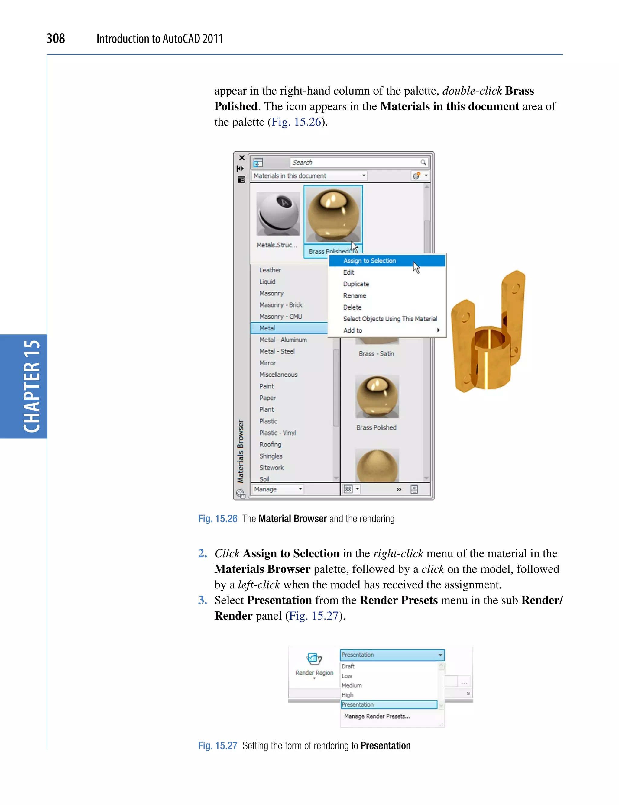
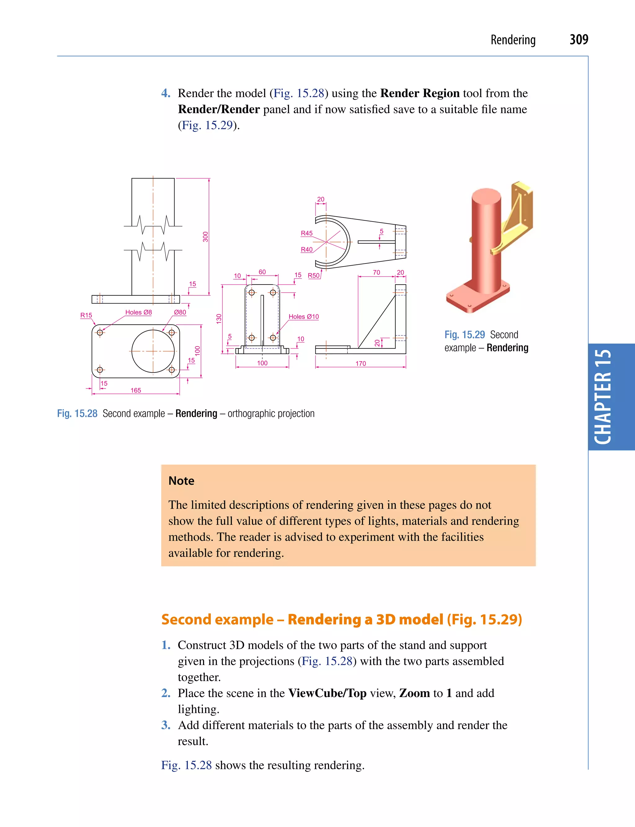
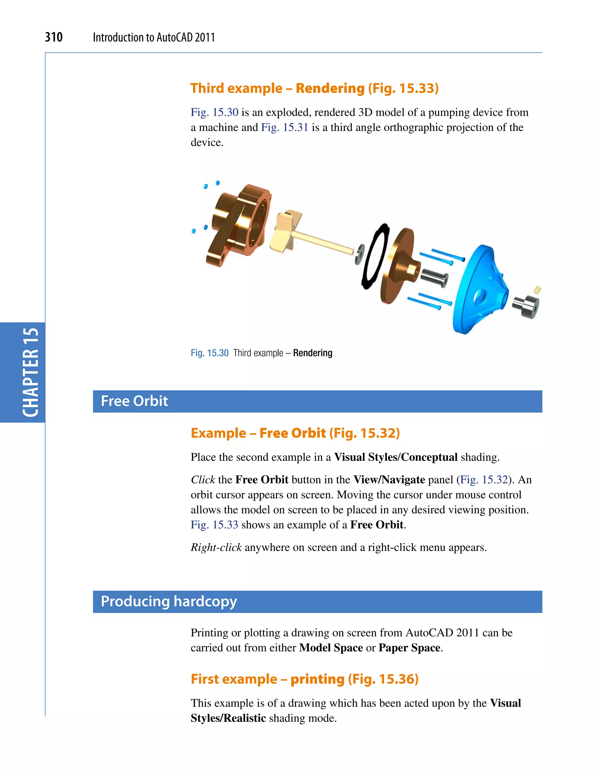
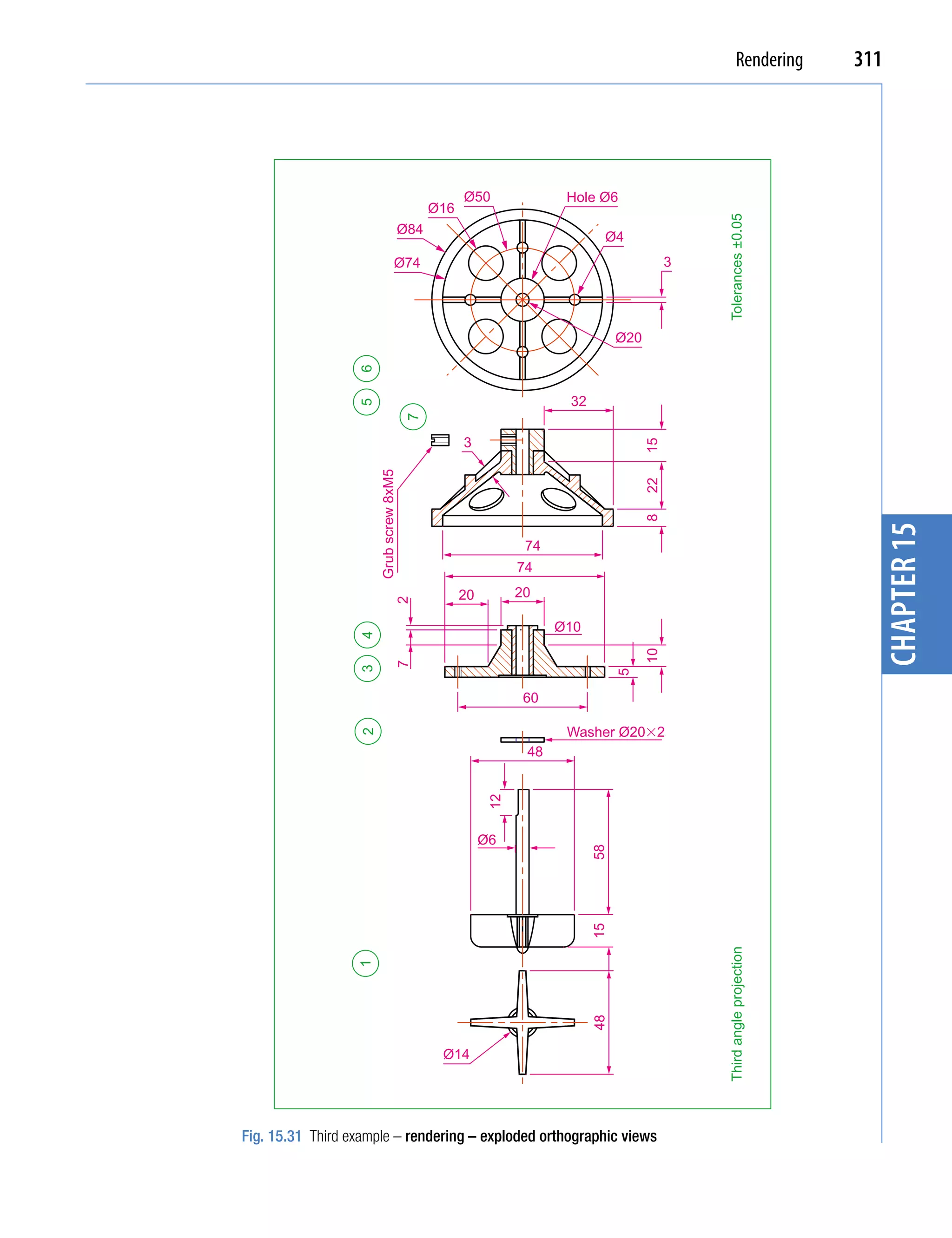
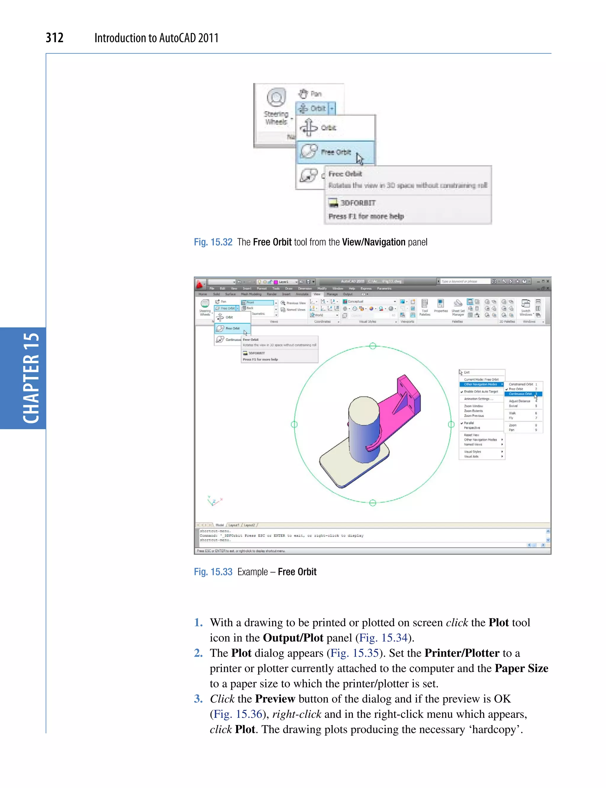
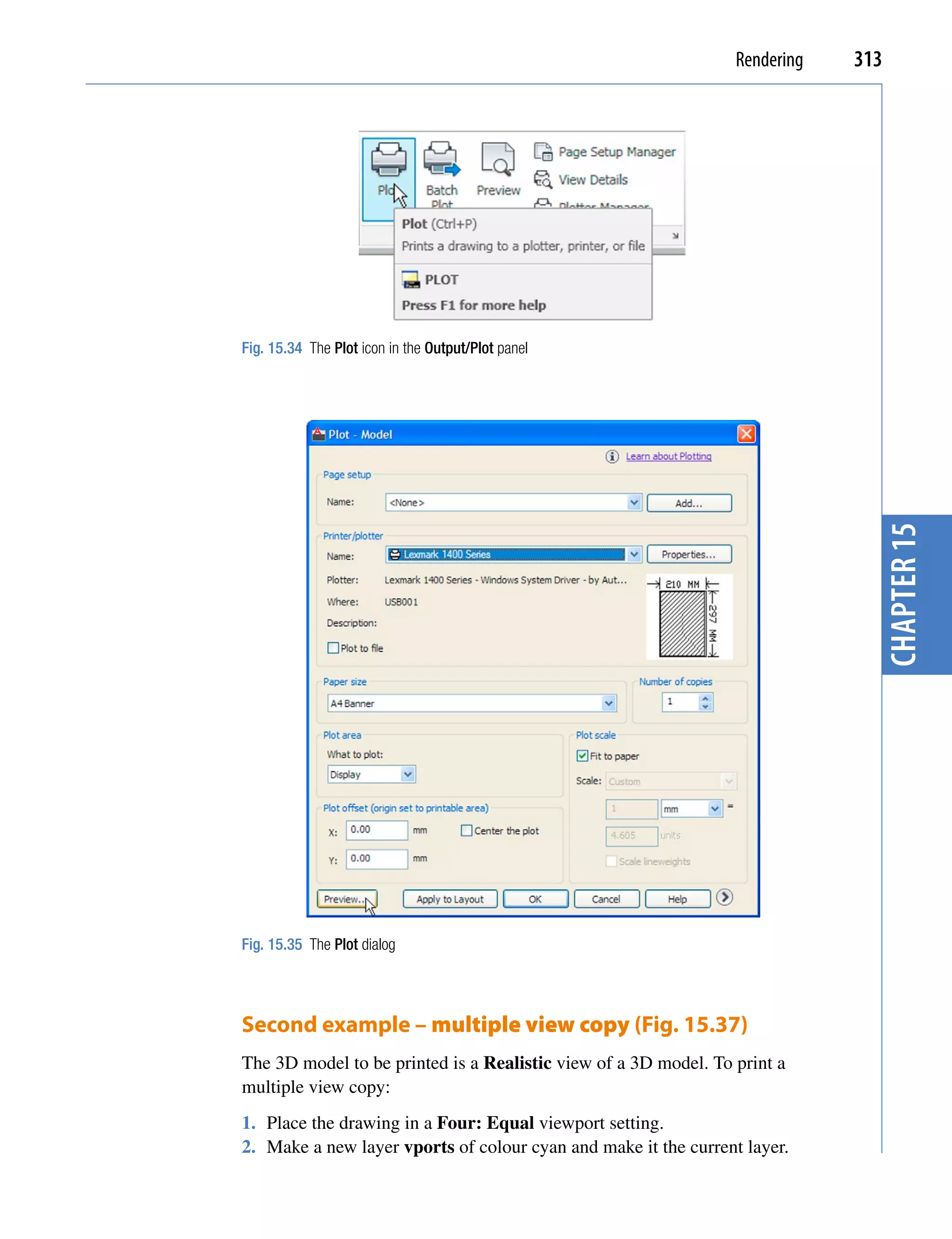
![chapter 15 314 Introduction to AutoCAD 2011
Fig. 15.36 First example – Print Preview – printing a single copy
Fig. 15.37 Second example – multiple view copy
3. Click the Layout button in the status bar. At the command line:
Command: enter mv (MVIEW) right-click
MVIEW
Specify corner of viewport or [ON/OFF/Fit/
Shadeplot/Lock/Object/Polygonal/Restore/
LAyer/2/3/4] <Fit>: enter r (Restore)
right-click](https://image.slidesharecdn.com/introductiontoautocad2011-100614022653-phpapp02/75/Introduction-to-AutoCad-2011-306-2048.jpg)
![Rendering 315
Enter viewport configuration name or [?]
<*Active>: right-click
Specify first corner or [Fit] <Fit>: right-click
Command:
The drawing appears in Paper Space. The views of the 3D model appear
each within a cyan outline in each viewport.
4. Turn layer vports off. The cyan outlines of the viewports disappear.
5. Click the Plot tool icon in the Output/Plot toolbar. Make sure the
correct Printer/Plotter and Paper Size settings are selected and click
the Preview button of the dialog.
6. If the preview is satisfactory (Fig. 15.37), right-click and from the
right-click menu click Plot. The drawing plots to produce the required
four-viewport hardcopy.
saving and opening 3D model drawings
chapter 15
3D model drawings are saved and/or opened in the same way as are
2D drawings. To save a drawing click Save As… in the File drop-down
menu and save the drawing in the Save Drawing As dialog by entering a
drawing file name in the File Name field of the dialog before clicking the
Save button. To open a drawing which has been saved click Open… in the
File drop-down menu, and in the Select File dialog which appears select a
file name from the file list.
There are differences between saving a 2D and a 3D drawing, in that when
3D model drawing is shaded by using a visual style from the Home/View
panel, the shading is saved with the drawing.
camera
Example – Camera shot in room scene
This example is of a camera being used in a room in which several chairs,
stools and tables have been placed. Start by constructing one of the chairs.
Constructing one of the chairs
1. In a Top view construct a polyline from an ellipse (after setting pedit to 1),
trimmed in half, then offset and formed into a single pline using pedit.
2. Construct a polyline from a similar ellipse, trimmed in half, then
formed into a single pline using pedit.](https://image.slidesharecdn.com/introductiontoautocad2011-100614022653-phpapp02/75/Introduction-to-AutoCad-2011-307-2048.jpg)
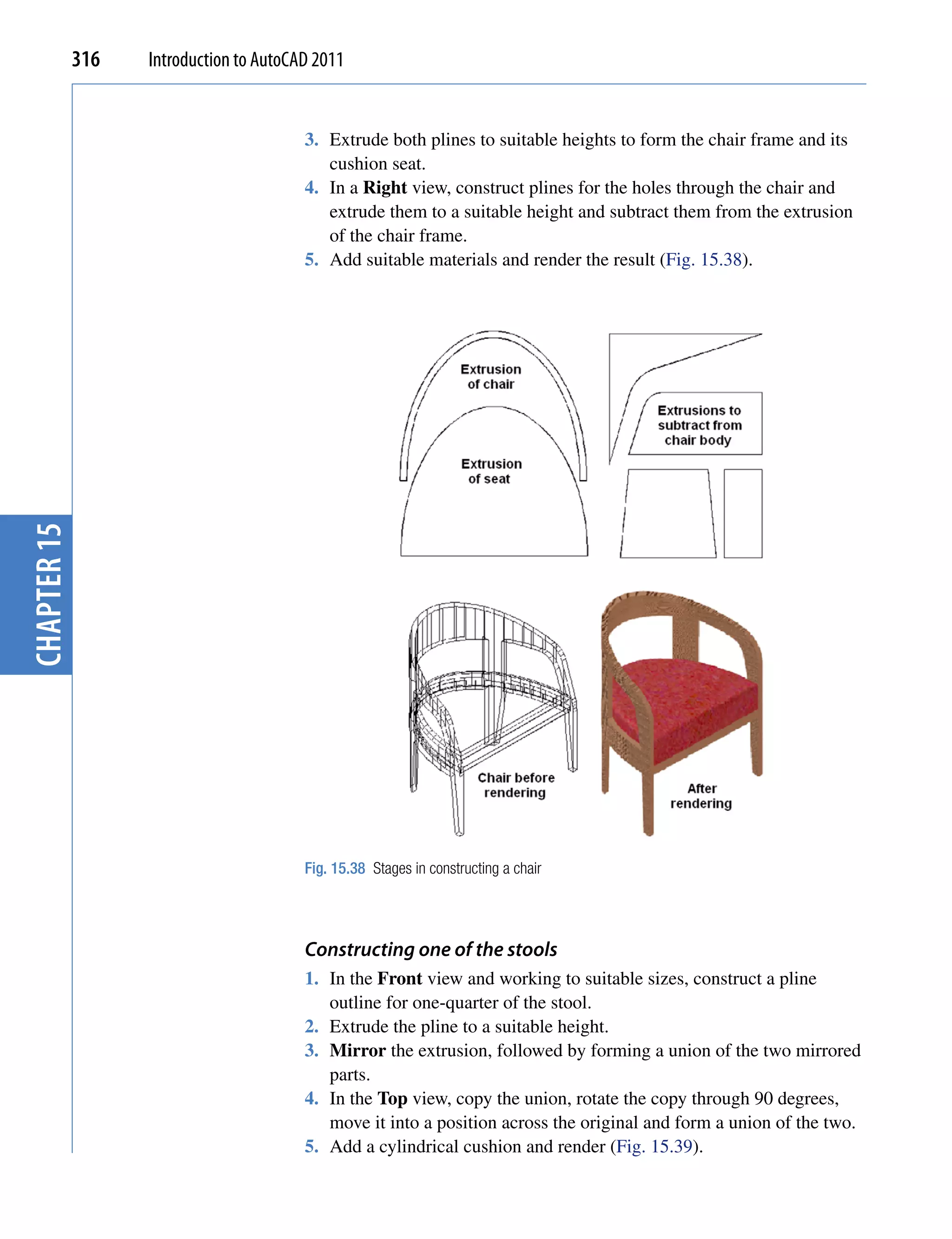
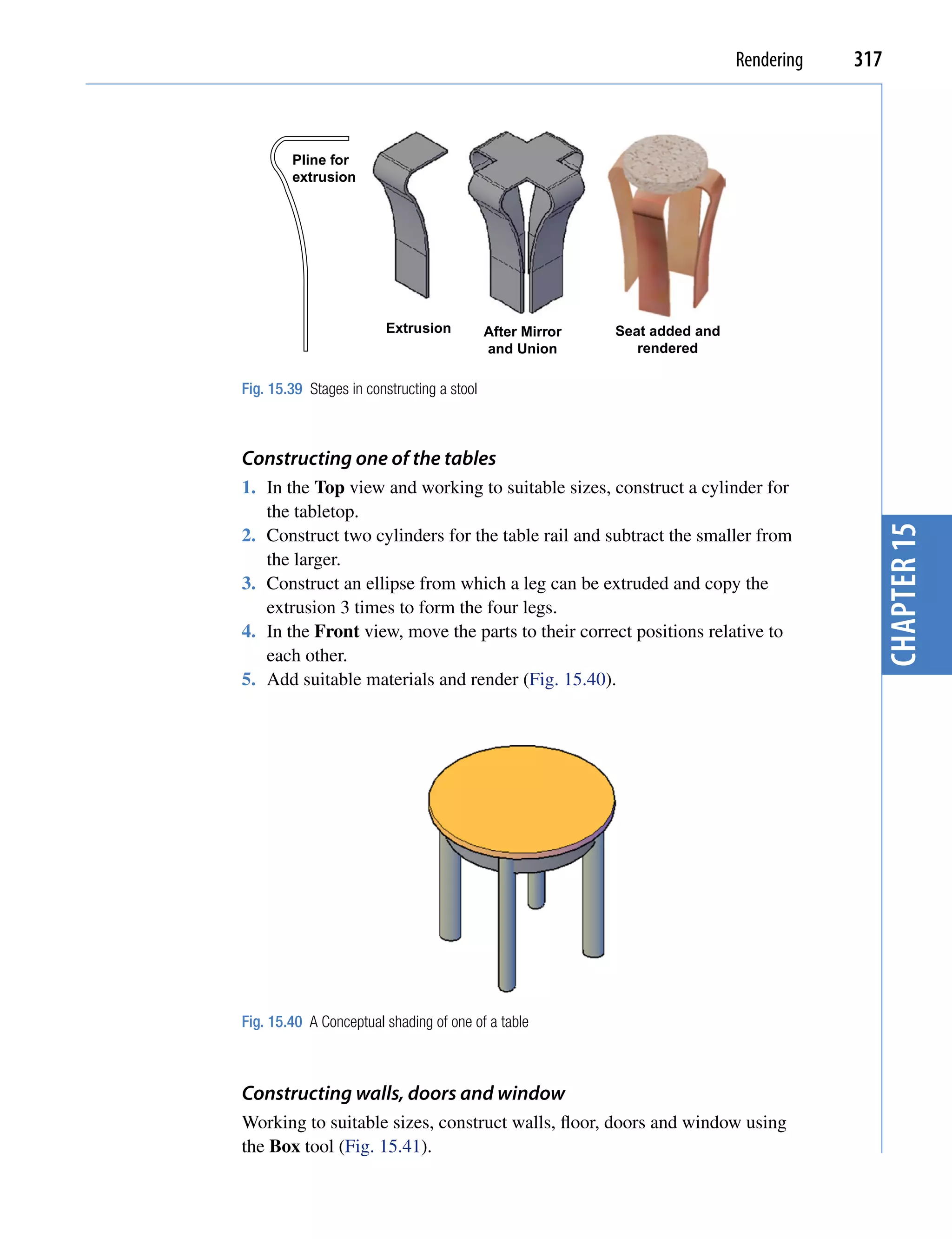
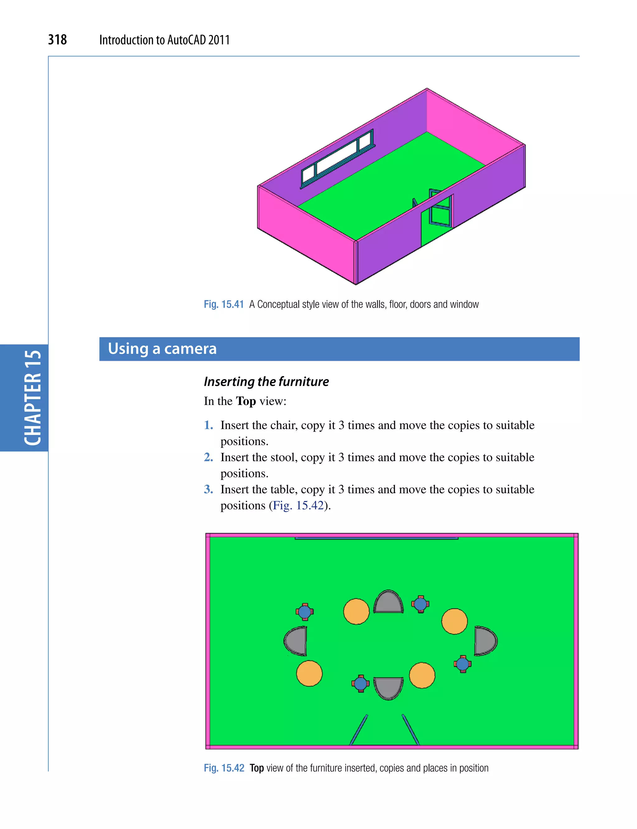
![Rendering 319
Adding lights
1. Place a 59 W 8 ft fluorescent light central to the room just below the
top of the wall height.
2. Place a Point light in the bottom right-hand central corner of the room
(Fig. 15.43).
chapter 15
Fig. 15.43 Two lights placed in the room
Placing a camera
1. Place the scene in the Front view.
2. Select Create Camera from the Render/Camera panel or from the
View drop-down menu (Fig. 15.44). The command line shows:
Command: _camera
Current camera settings: Height=0 Lens
Length=80 mm
Specify camera location: pick a position
Specify target location: drag to end of the cone
into position
Enter an option [?/Name/LOcation/Height/Target/
LEns/Clipping/View/eXit] <eXit>: enter
le (LEns) right-click
Specify lens length in mm <80>: enter 55
right-click](https://image.slidesharecdn.com/introductiontoautocad2011-100614022653-phpapp02/75/Introduction-to-AutoCad-2011-311-2048.jpg)
![320 Introduction to AutoCAD 2011
Enter an option [?/Name/LOcation/Height/Target/
LEns/Clipping/View/eXit] <eXit>: n
Enter name for new camera <Camera2>: right-click
-accepts name (Camera1)
Enter an option [?/Name/LOcation/Height/Target/
LEns/Clipping/View/eXit] <eXit>: right-click
Command:
And the camera will be seen in position (Fig. 15.45).
chapter 15
Fig. 15.44 Selecting Create Camera from the View drop-down menu
Fig. 15.45 The camera in position](https://image.slidesharecdn.com/introductiontoautocad2011-100614022653-phpapp02/75/Introduction-to-AutoCad-2011-312-2048.jpg)
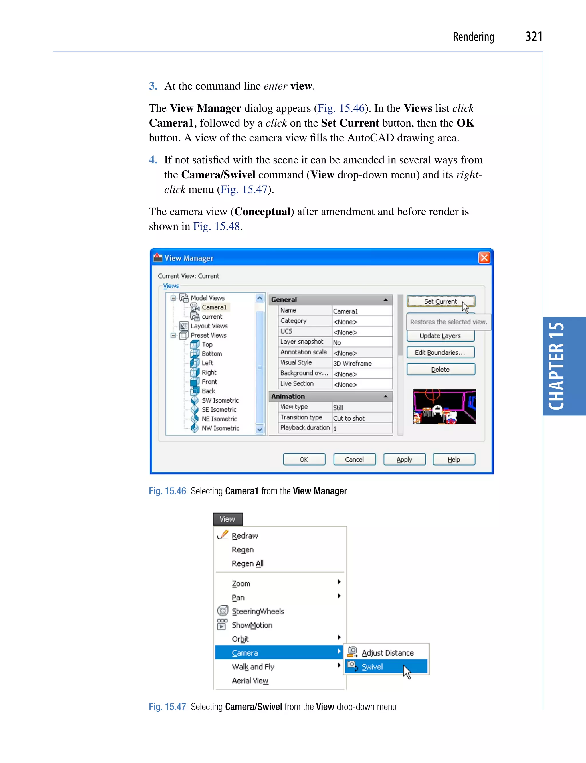
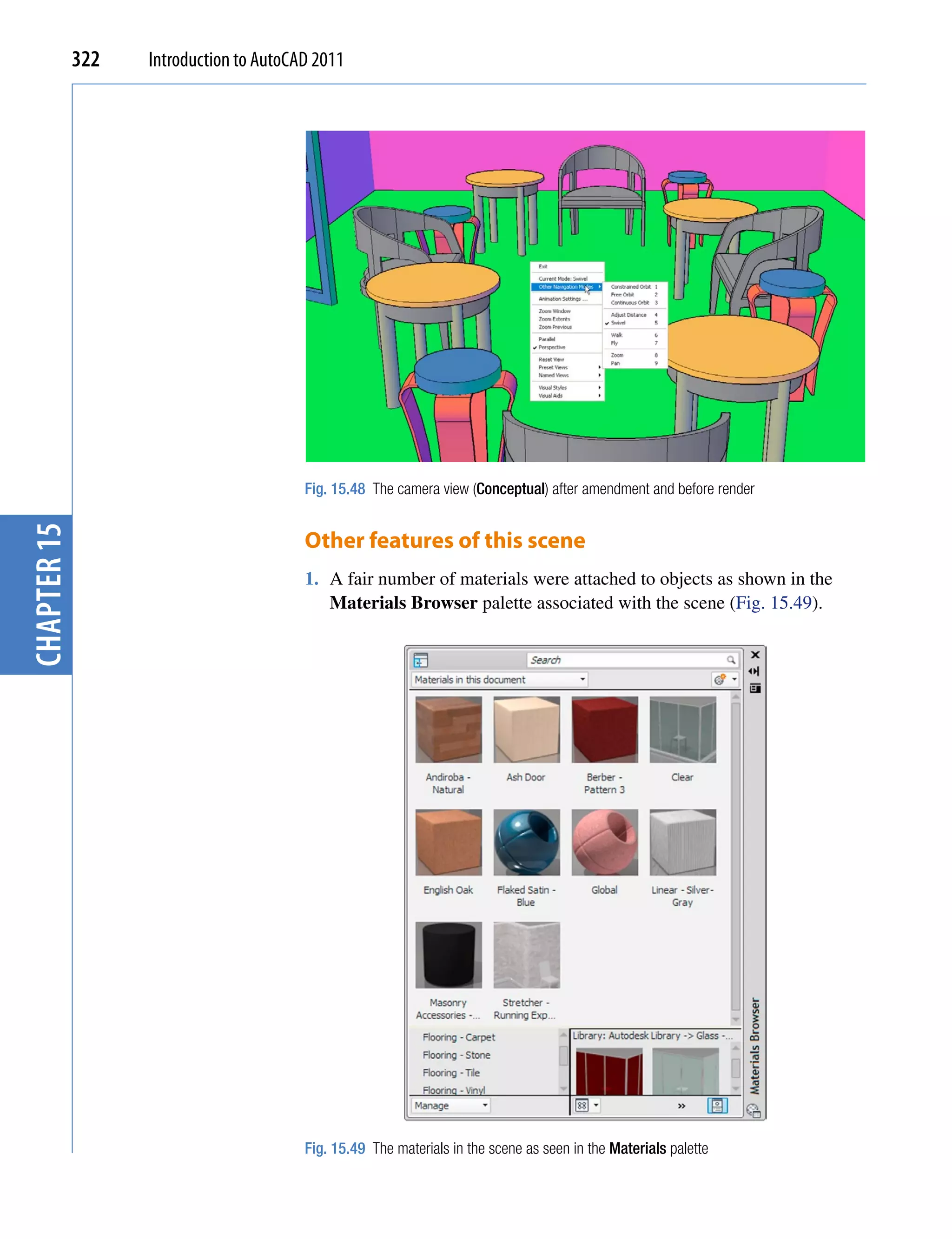
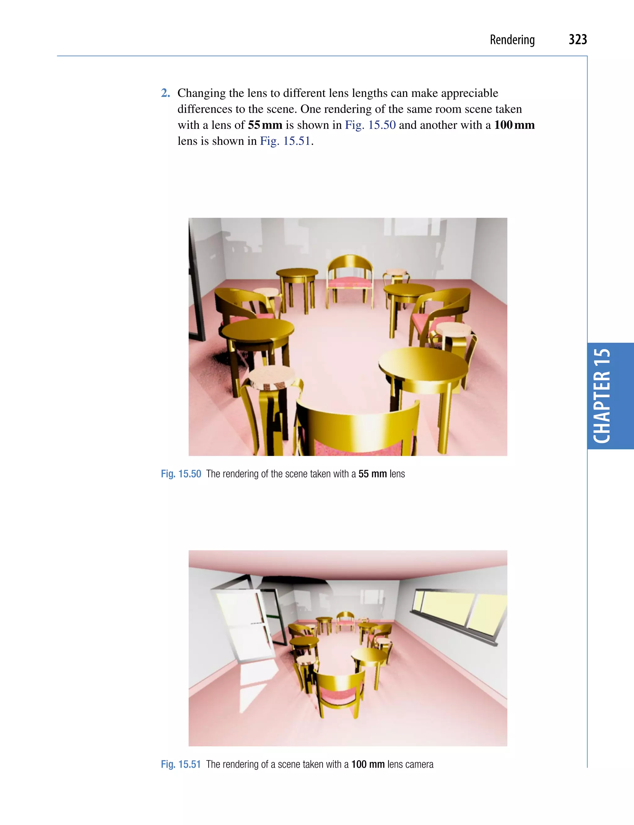

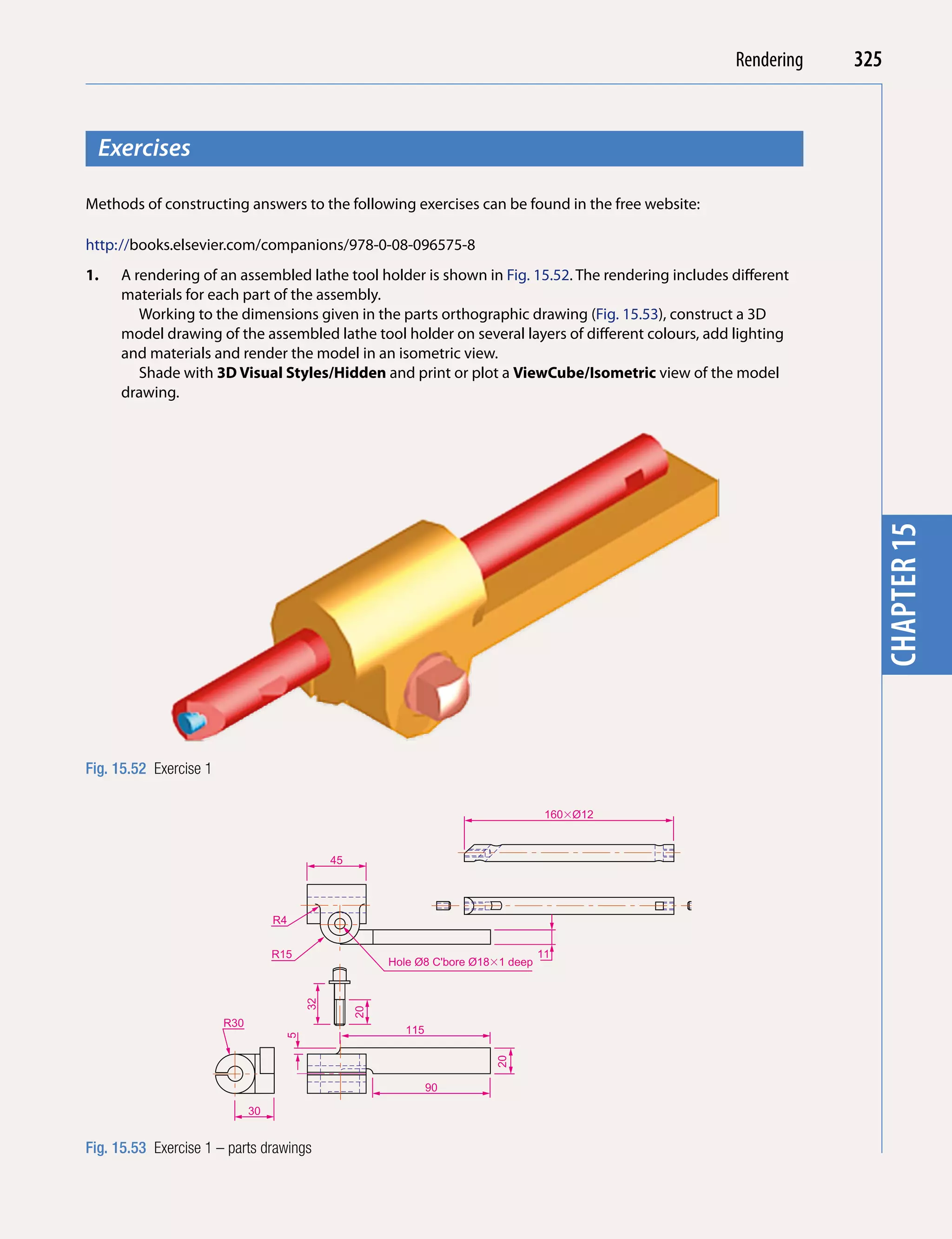
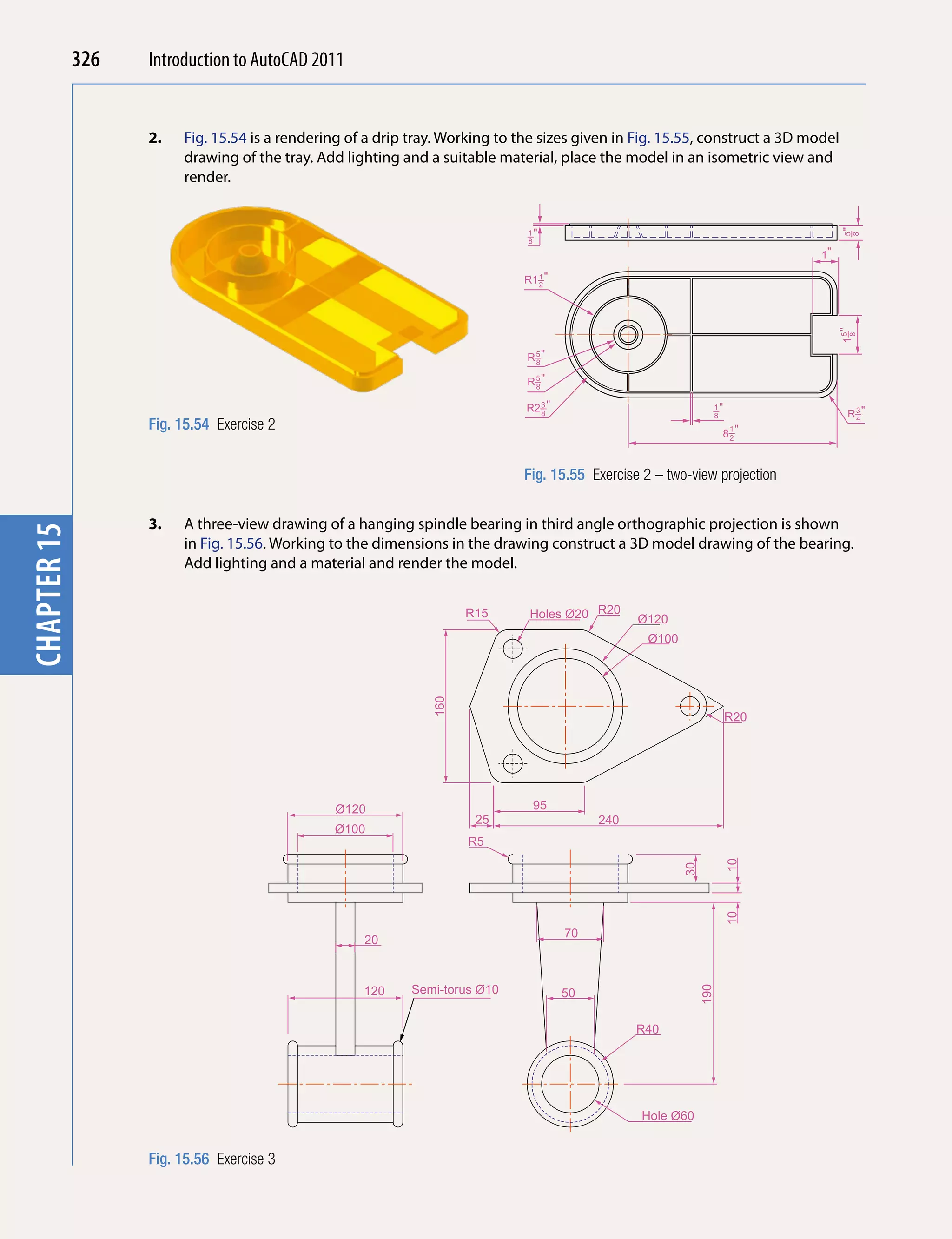

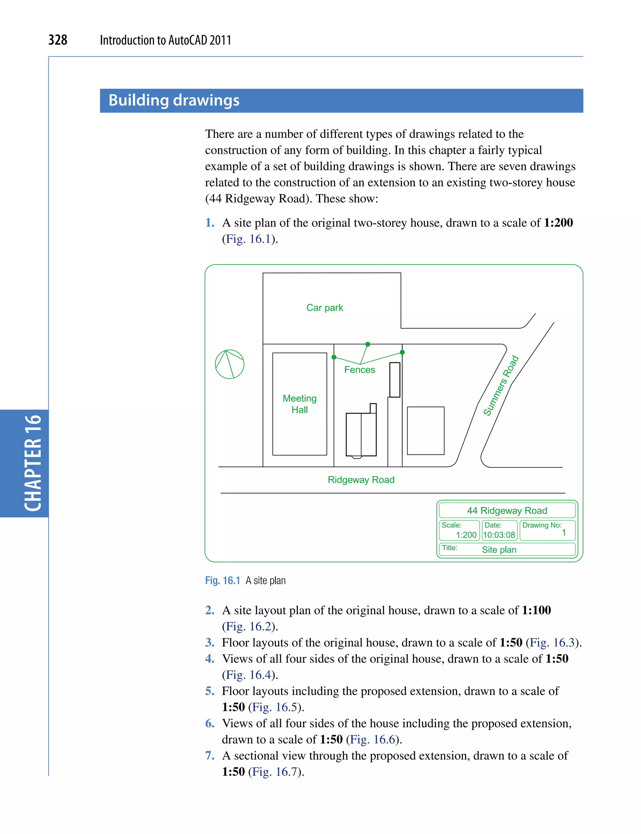
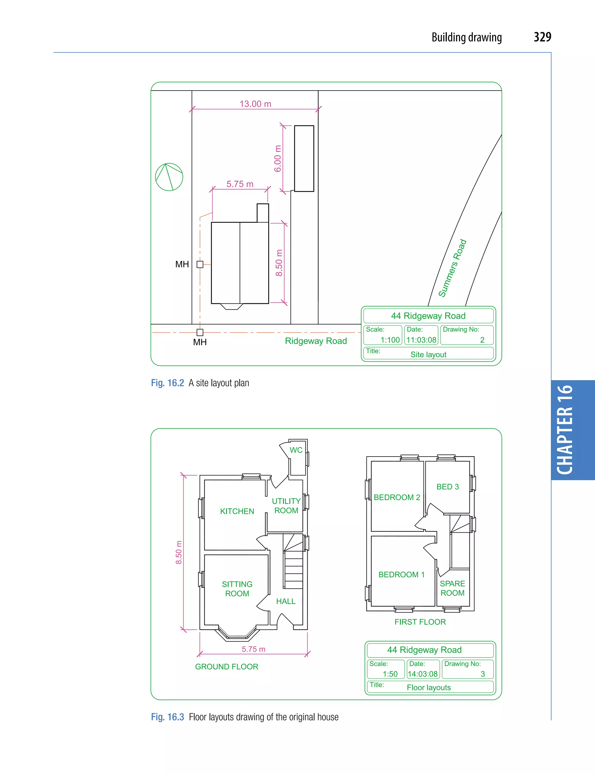
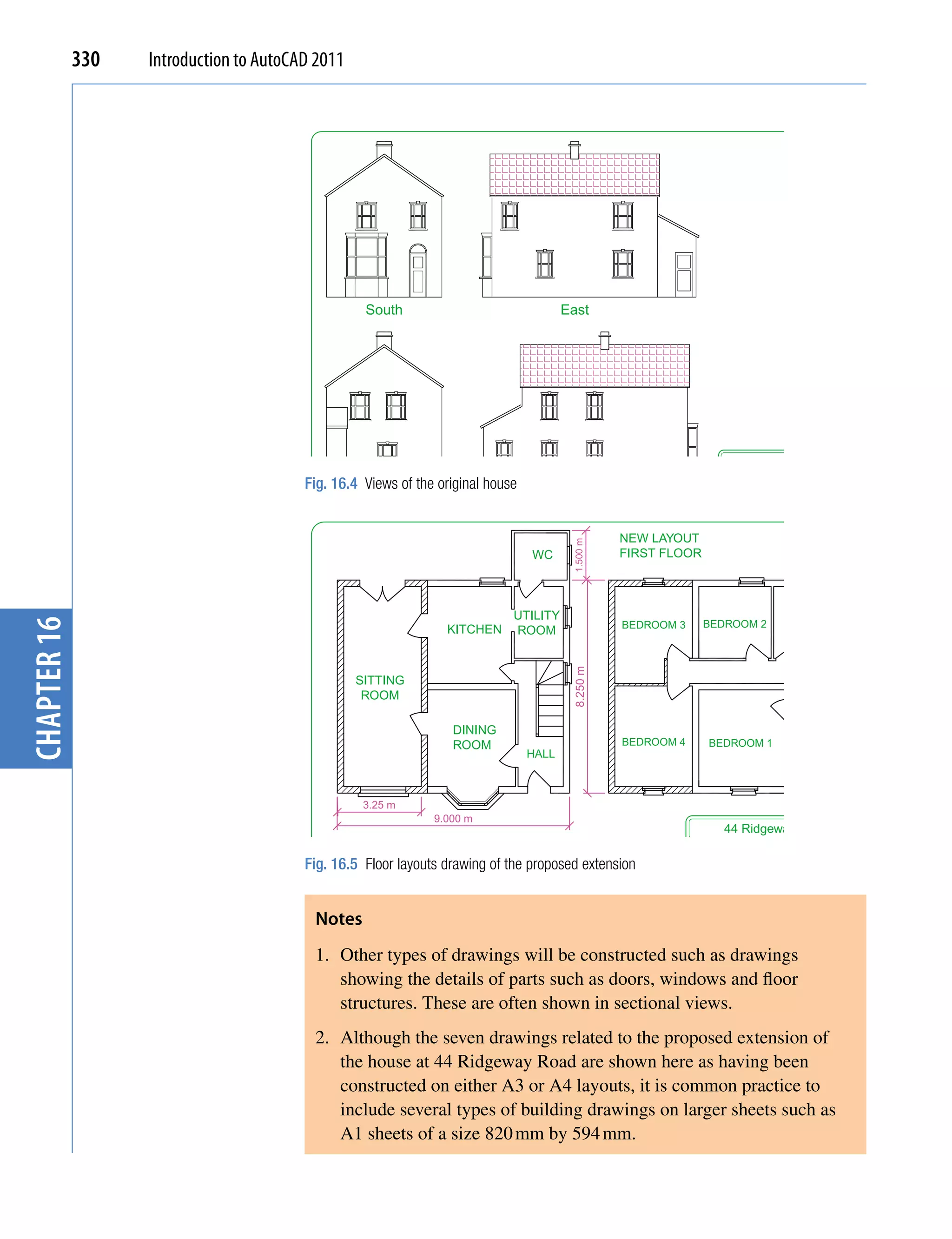
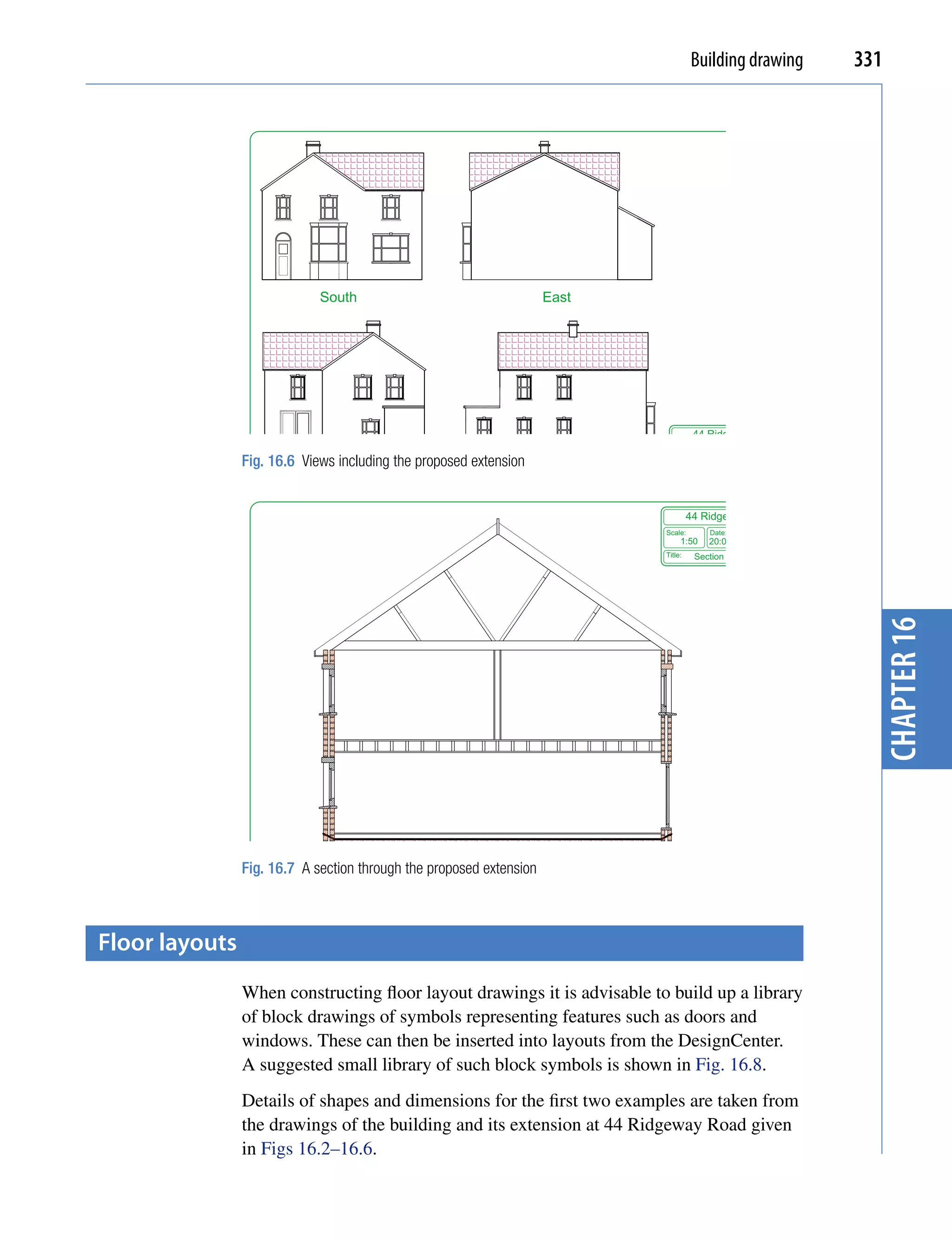
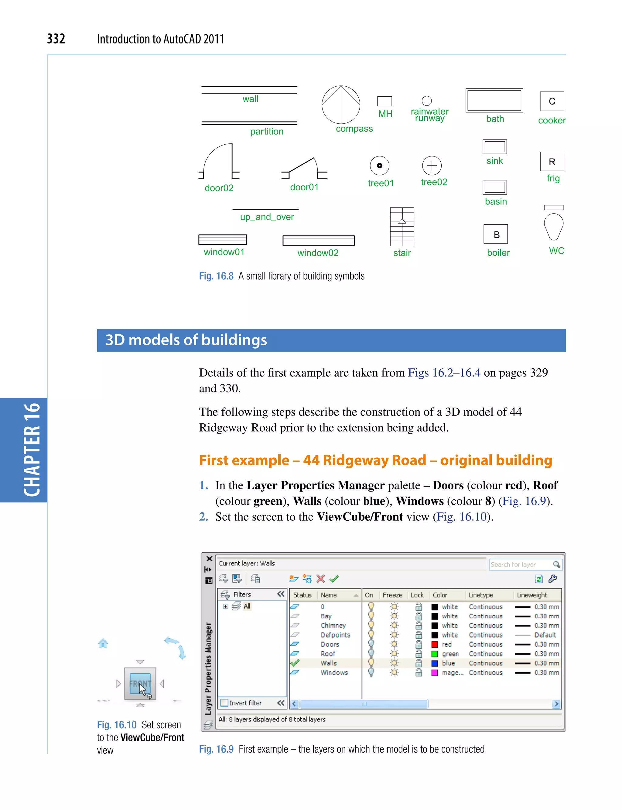
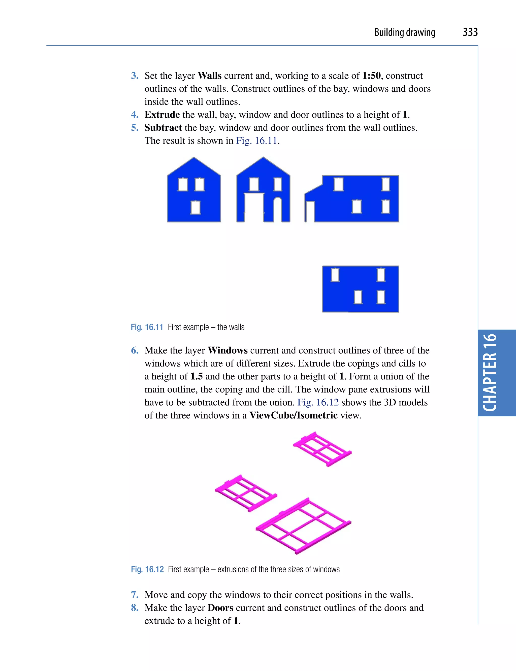
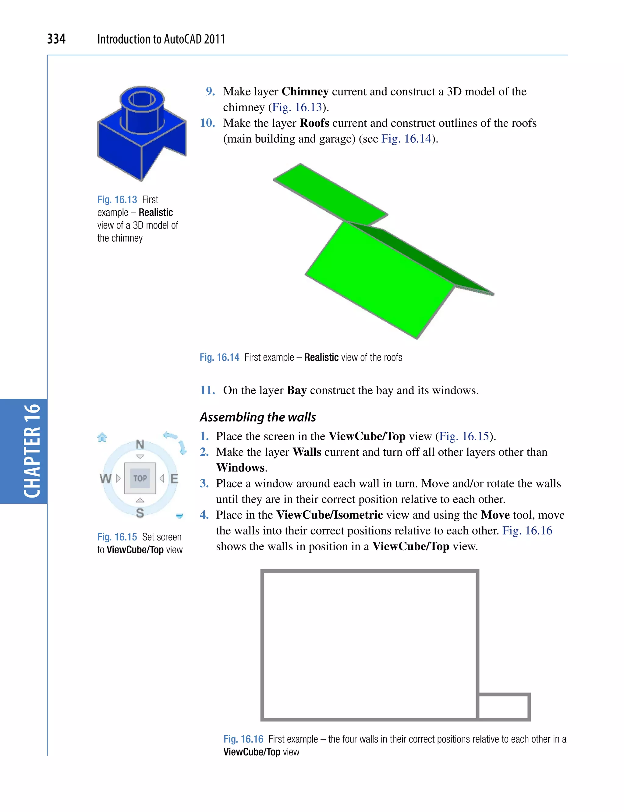
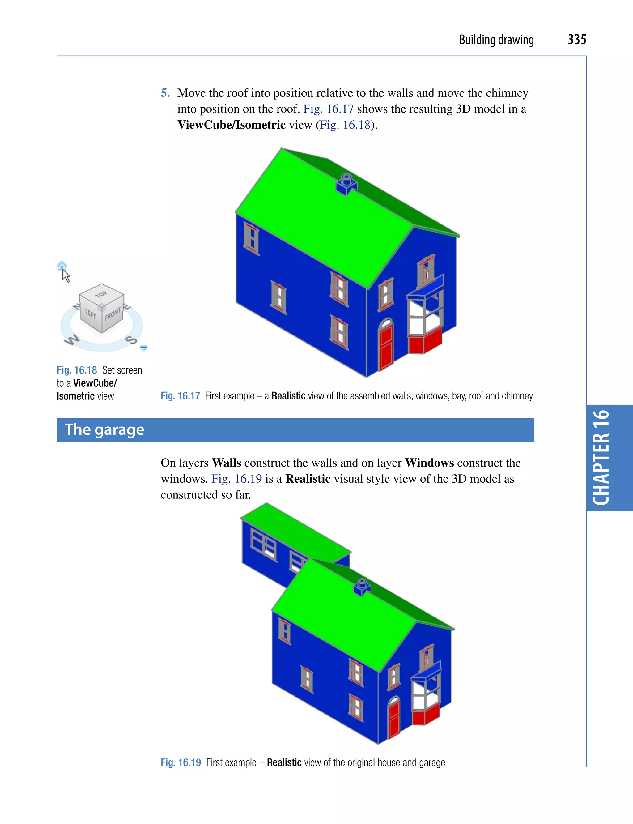
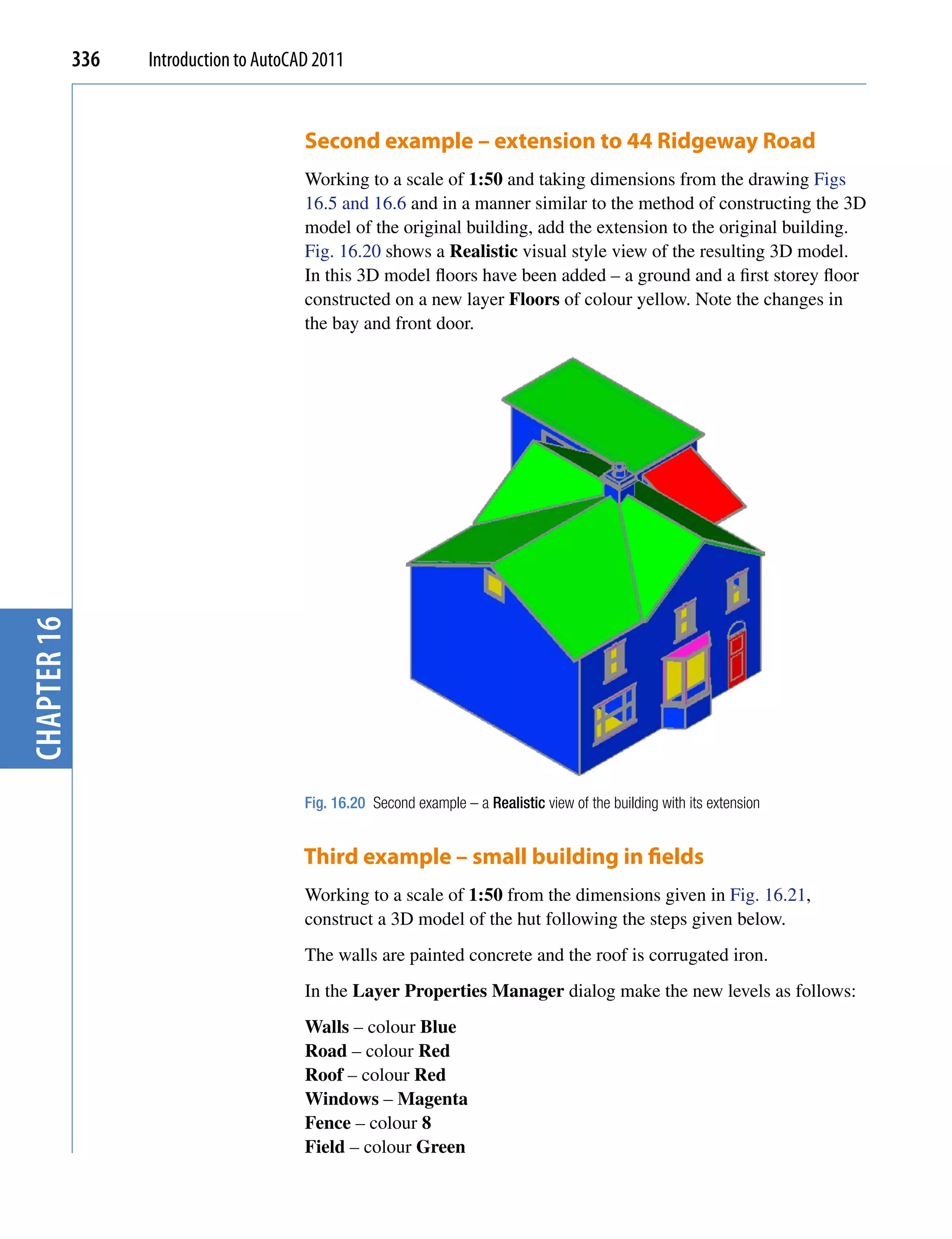
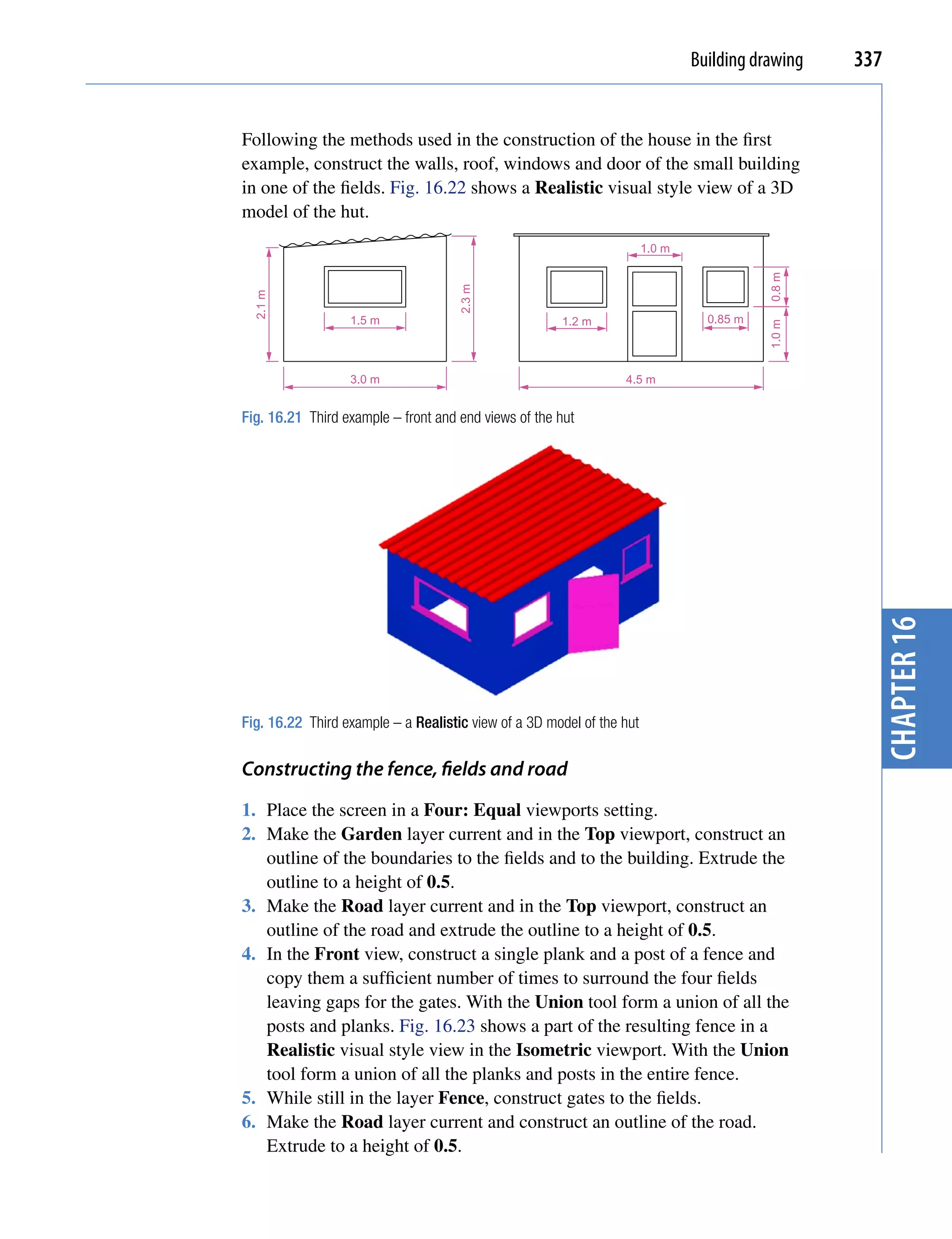
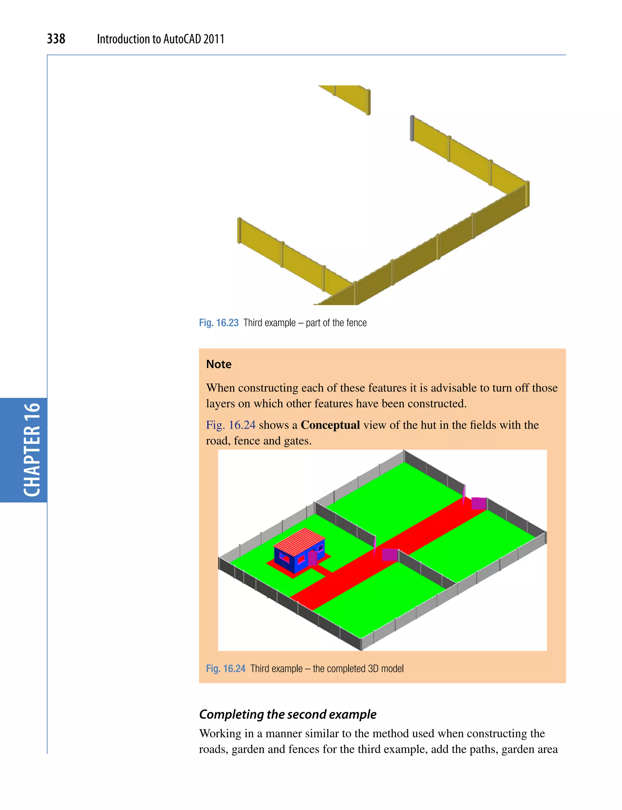

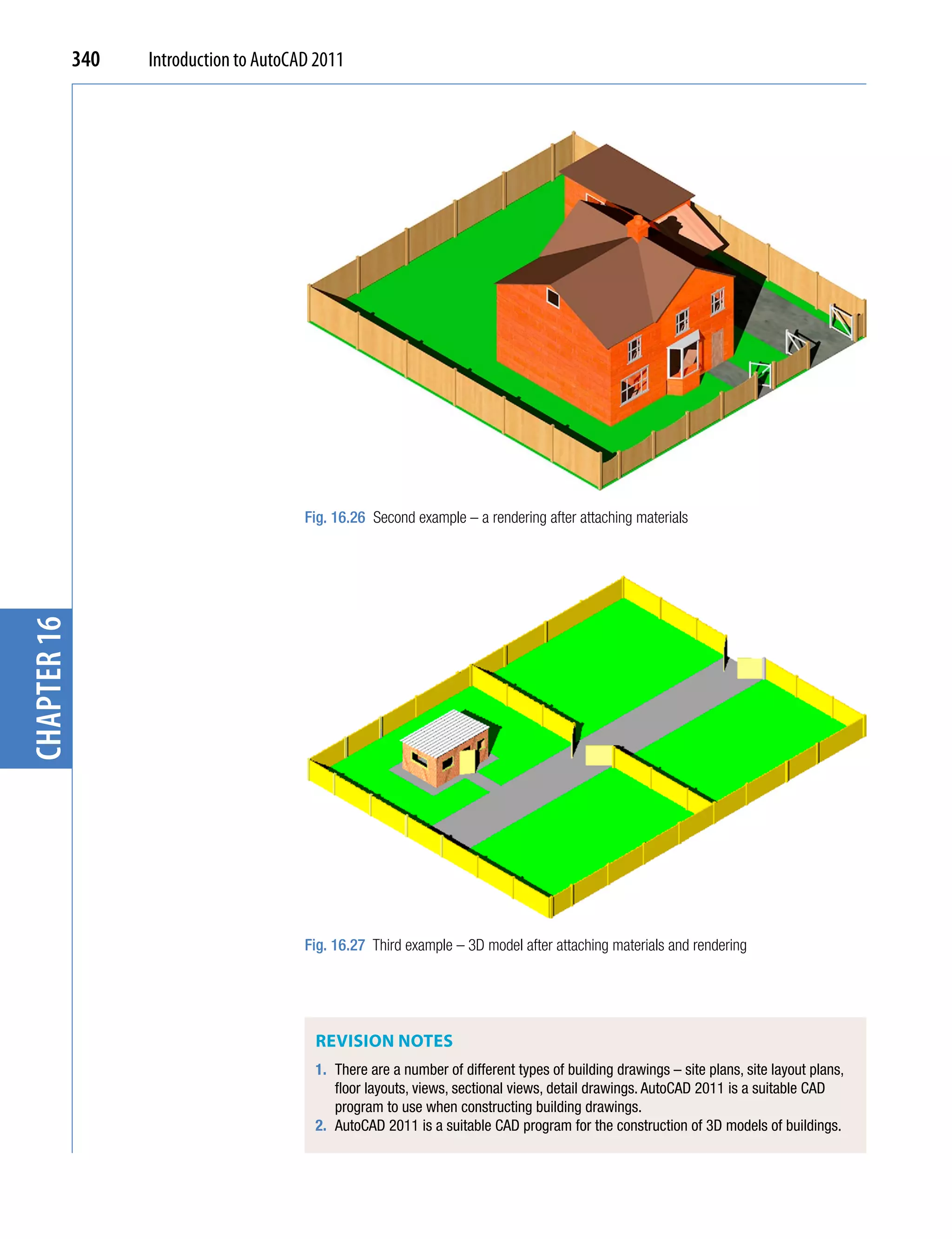
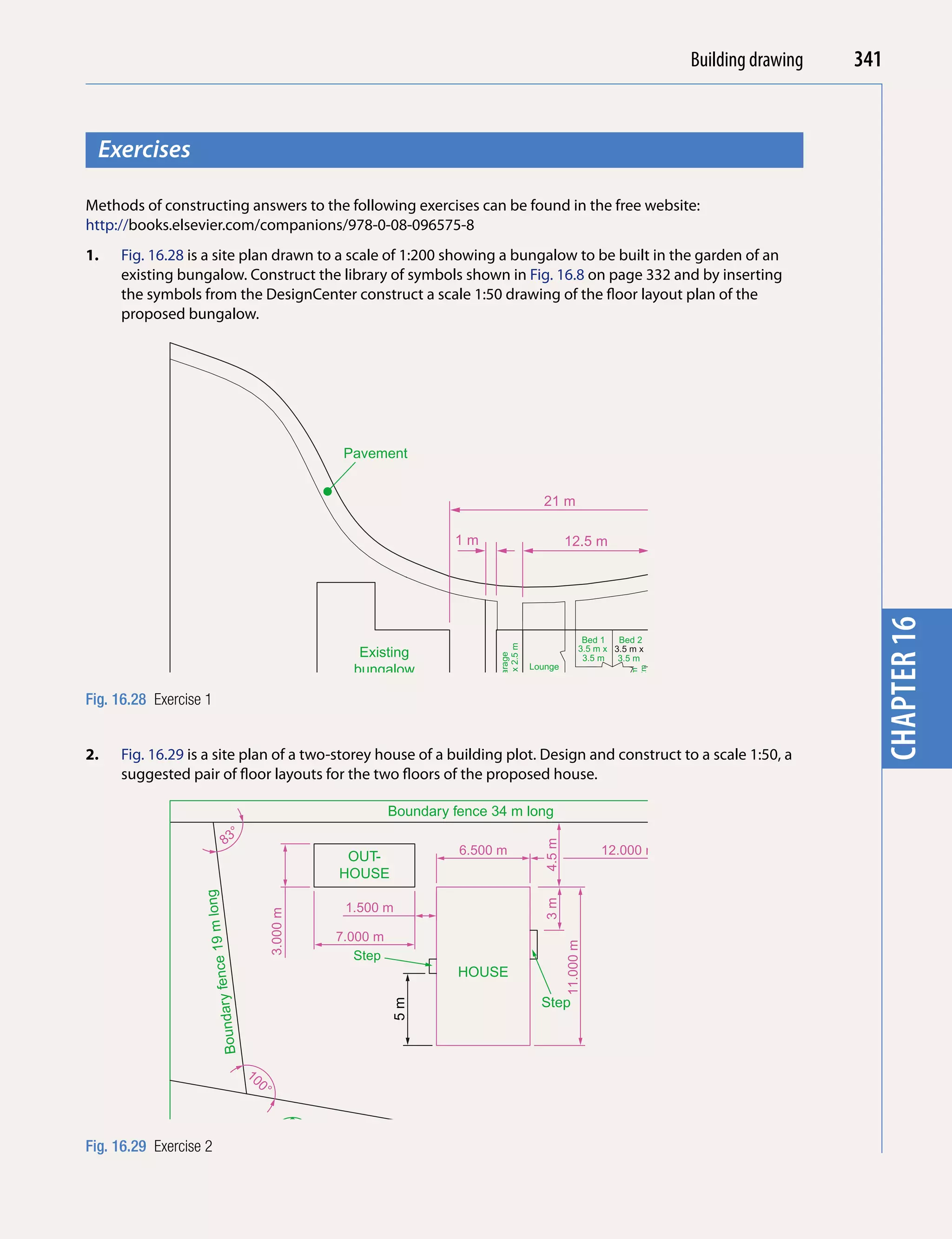
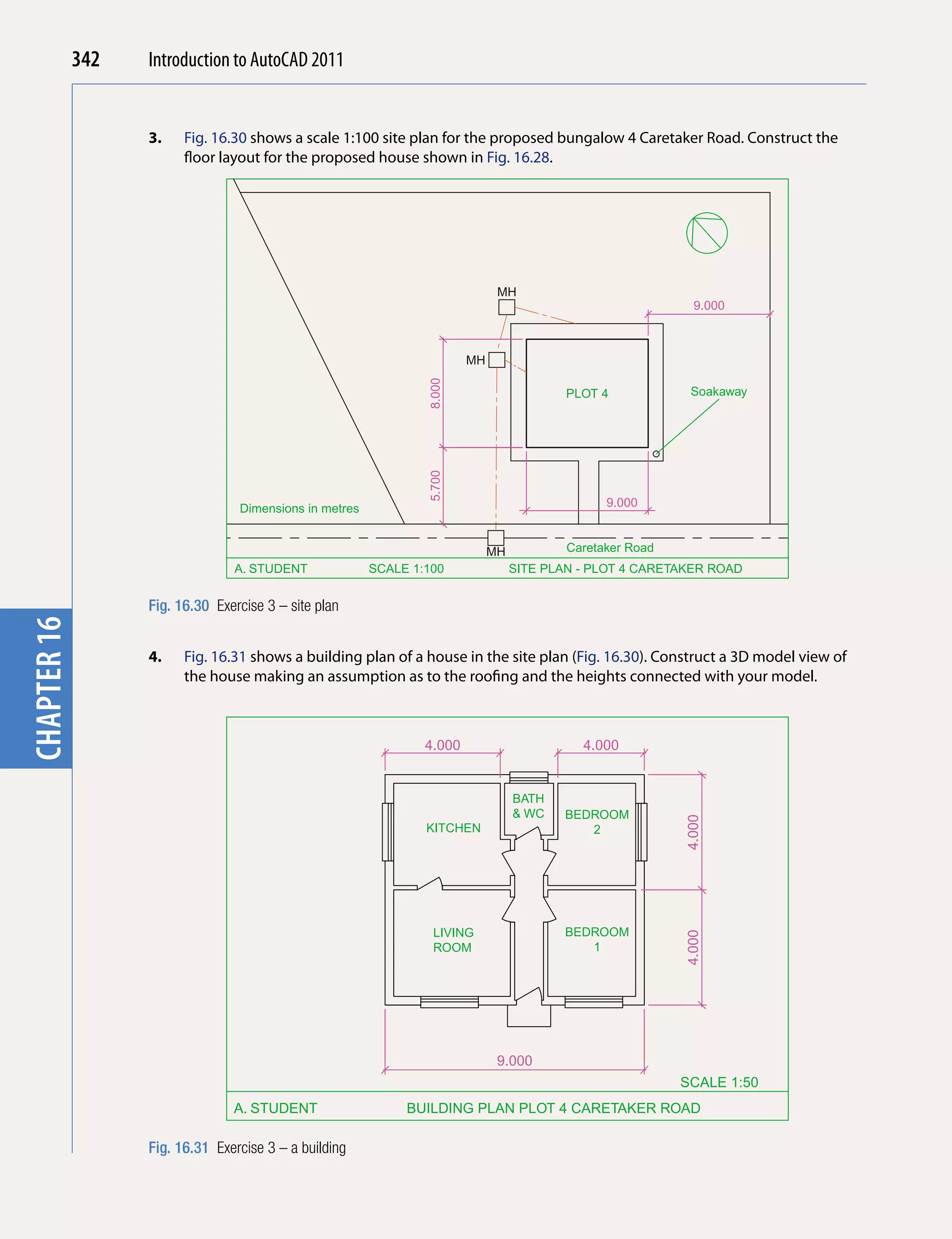
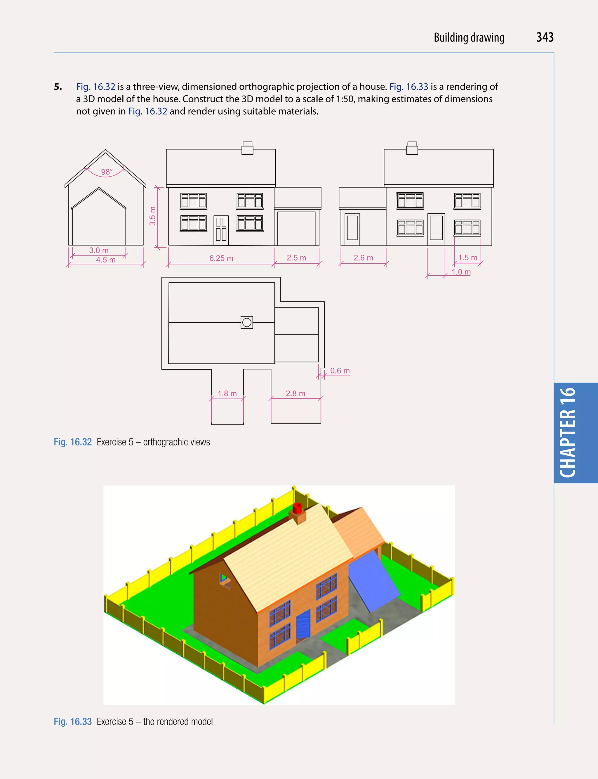
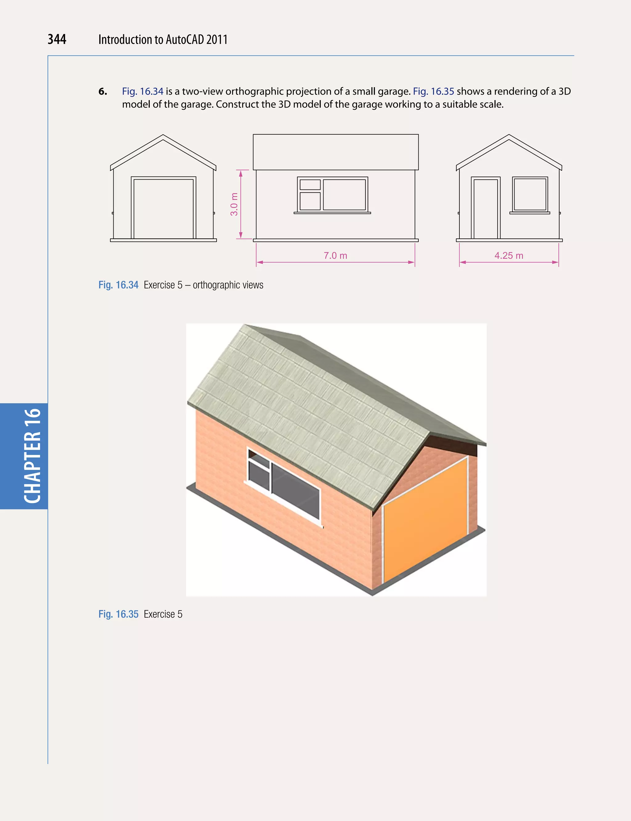
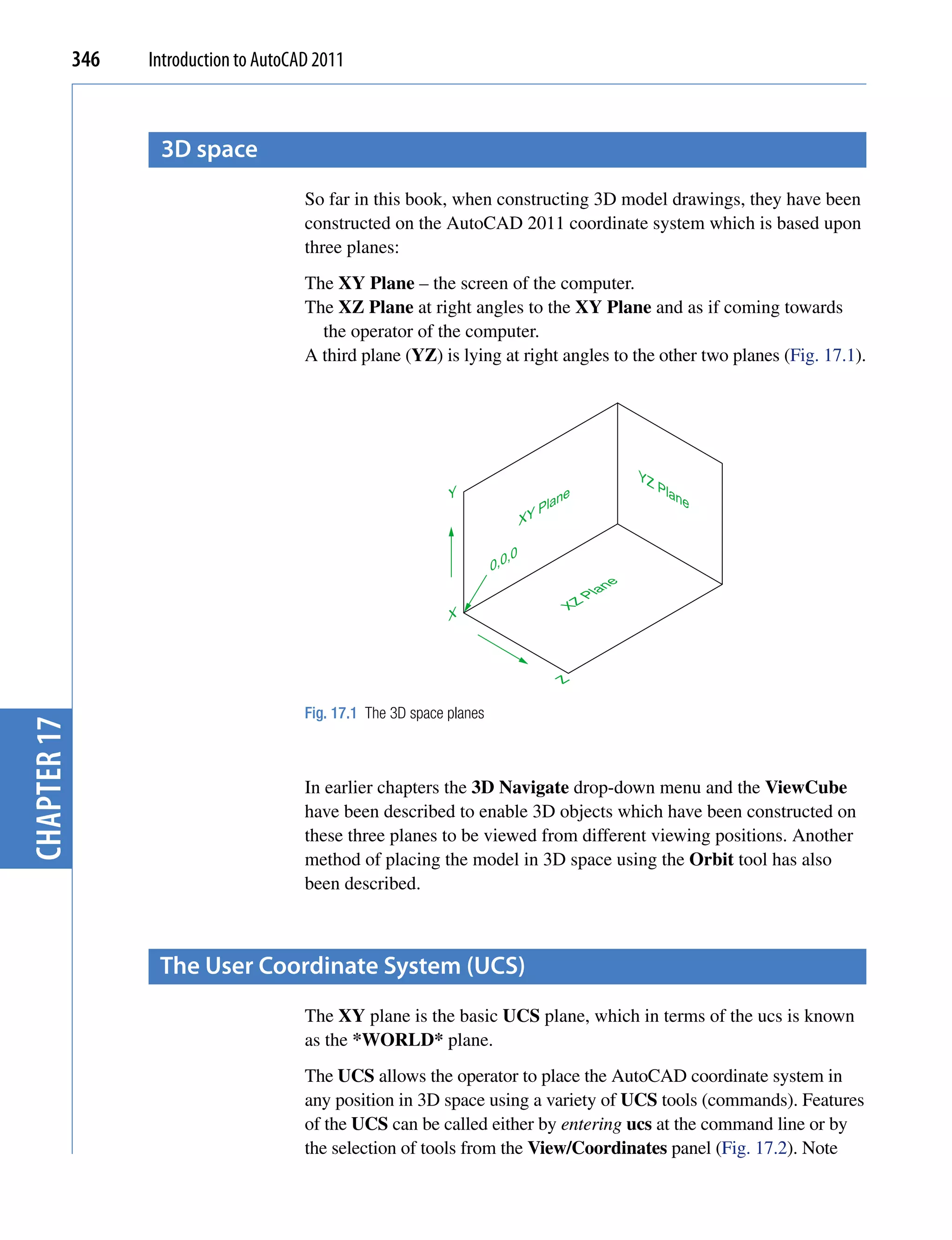
![Three-dimensional space 347
Fig. 17.2 The View/
Coordinates panel
Fig. 17.3 The drop-down menu from World in the panel
that a click on World in the panel brings a drop-down menu from which
other views can be selected (Fig. 17.3).
If ucs is entered at the command line, it shows:
Command: enter ucs right-click
Current ucs name: *WORLD*
Specify origin of UCS or [Face/NAmed/OBject/
Previous/View/World/X/Y/Z/ZAxis] <World>:
chapter 17
And from these prompts selection can be made.
the variable UcsfoLLoW
UCS planes can be set from using the methods shown in Figs 17.2 and
17.3 or by entering ucs at the command line. No matter which method is
used, the variable UCSFOLLOW must first be set on as follows:
Command: enter ucsfollow right-click
Enter new value for UCSFOLLOW <0>: enter 1
right-click
Command:
the UCS icon
The UCS icon indicates the directions in which the three coordinate axes
X, Y and Z lie in the AutoCAD drawing. When working in 2D, only the](https://image.slidesharecdn.com/introductiontoautocad2011-100614022653-phpapp02/75/Introduction-to-AutoCad-2011-339-2048.jpg)
![348 Introduction to AutoCAD 2011
X and Y axes are showing, but when the drawing area is in a 3D view all
three coordinate arrows are showing, except when the model is in the XY
plane. The icon can be turned off as follows:
Command: enter ucsicon right-click
Enter an option [ON/OFF/All/Noorigin/ORigin/
Properties] <ON>:
To turn the icon off, enter off in response to the prompt line and the icon
disappears from the screen.
The appearance of the icon can be changed by entering p (Properties) in
response to the prompt line. The UCS Icon dialog appears in which changes
can be made to the shape, line width and colour of the icon if wished.
Types of UCS icon
The shape of the icon can be varied partly when changes are made in the
UCS Icon dialog but also according to whether the AutoCAD drawing
area is in 2D, 3D or Paper Space (Fig. 17.4).
chapter 17
Fig. 17.4 Types of UCS icon
examples of changing planes using the Ucs
First example – changing UCS planes (Fig. 17.6)
1. Set UCSFOLLOW to 1 (ON).
2. Make a new layer colour Red and make the layer current. Place the
screen in ViewCube/Front and Zoom to 1.
3. Construct the pline outline (Fig. 17.5) and extrude to 120 high.
4. Place in ViewCube/Isometric view and Zoom to 1.
5. With the Fillet tool, fillet corners to a radius of 20.](https://image.slidesharecdn.com/introductiontoautocad2011-100614022653-phpapp02/75/Introduction-to-AutoCad-2011-340-2048.jpg)
![Three-dimensional space 349
15
0
15
°
120
160
15
Fig. 17.5 First example – Changing UCS planes – pline for extrusion
6. At the command line:
Command: enter ucs right-click
Current ucs name: *WORLD*
Specify origin of UCS or [Face/NAmed/OBject/
Previous/View/World/X/Y/Z/ZAxis] <World>:
enter f (Face) right-click
Select face of solid object: pick the sloping
face – its outline highlights
Enter an option [Next/Xflip/Yflip] <accept>:
right-click
Regenerating model.
Command:
And the 3D model changes its plane so that the sloping face is now on
chapter 17
the new UCS plane. Zoom to 1.
7. On this new UCS, construct four cylinders of radius 7.5 and height − 15
(note the minus) and subtract them from the face.
8. Enter ucs at the command line again and right-click to place the model
in the *WORLD* UCS.
9. Place four cylinders of the same radius and height into position in the
base of the model and subtract them from the model.
Fig. 17.6 First 10. Place the 3D model in a ViewCube/Isometric view and set in the
example – Changing Home/View/Conceptual visual style (Fig. 17.6).
UCS planes
Second example – UCS (Fig. 17.9)
The 3D model for this example is a steam venting valve – a two-view third
angle projection of the valve is shown in Fig. 17.7.
1. Make sure that UCSFOLLOW is set to 1.
2. Place in the UCS *WORLD* view. Construct the 120 square plate at
the base of the central portion of the valve. Construct five cylinders for
the holes in the plate. Subtract the five cylinders from the base plate.](https://image.slidesharecdn.com/introductiontoautocad2011-100614022653-phpapp02/75/Introduction-to-AutoCad-2011-341-2048.jpg)
![350 Introduction to AutoCAD 2011
Octagon edge length 40
25
SQ 120
SQ 80
90
Hole Ø70
35
R20
10 40 Sq head bolts M10
Holes Ø10 60
20
10
10
40
60
Hole Ø30
R5 R10
Fig. 17.7 Second example UCS – The orthographic projection of a steam venting valve
3. Construct the central part of the valve – a filleted 80 square extrusion
with a central hole.
4. At the command line:
Command: enter ucs right-click
chapter 17
Current ucs name: *WORLD*
Specify origin of UCS or [Face/NAmed/OBject/
Previous/View/World/X/Y/Z/ZAxis] <World>:
enter x right-click
Specify rotation angle about X axis <90>:
right-click
Command:
and the model assumes a Front view.
5. With the Move tool, move the central portion vertically up by 10.
6. With the Copy tool, copy the base up to the top of the central portion.
7. With the Union tool, form a single 3D model of the three parts.
8. Make the layer Construction current.
9. Place the model in the UCS *WORLD* view. Construct the separate
top part of the valve – a plate forming a union with a hexagonal plate
and with holes matching those of the other parts.
10. Place the drawing in the UCS X view. Move the parts of the top into
their correct positions relative to each other. With Union and Subtract
complete the part. This will be made easier if the layer 0 is turned off.](https://image.slidesharecdn.com/introductiontoautocad2011-100614022653-phpapp02/75/Introduction-to-AutoCad-2011-342-2048.jpg)
![Three-dimensional space 351
11. Turn layer 0 back on and move the top into its correct position relative
to the main part of the valve. Then with the Mirror tool, mirror the
top to produce the bottom of the assembly (Fig. 17.8).
12. While in the UCS X view construct the three parts of a 3D model of
the extrusion to the main body.
13. In the UCS *WORLD* view, move the parts into their correct position
relative to each other. Union the two filleted rectangular extrusions and
Fig. 17.8 Second the main body. Subtract the cylinder from the whole (Fig. 17.9).
example UCS – step 14. In the UCS X view, construct one of the bolts as shown in Fig. 17.10,
11 rendering
forming a solid of revolution from a pline. Then construct a head to
the bolt and with Union add it to the screw.
15. With the Copy tool, copy the bolt 7 times to give 8 bolts. With Move,
and working in the UCS *WORLD* and X views, move the bolts
into their correct positions relative to the 3D model.
16. Add suitable lighting and attach materials to all parts of the assembly
and render the model.
17. Place the model in the ViewCube/Isometric view.
Fig. 17.9 Second 18. Save the model to a suitable file name.
example UCS – steps 19. Finally move all the parts away from each other to form an exploded
12 and 13 rendering view of the assembly (Fig. 17.11).
5
Third example – UCS (Fig. 17.15)
20
1. Set UCSFOLLOW to 1.
Fig. 17.10 Second 2. Place the drawing area in the UCS X view.
chapter 17
example UCS – pline
for the bolt 3. Construct the outline (Fig 17.12) and extrude to a height of 120.
4. Click the 3 Point tool icon in the View/Coordinates
panel (Fig. 17.13):
Command: _ucs
Current ucs name: *WORLD*
Specify origin of UCS or [Face/NAmed/OBject/
Previous/View/World/X/Y/Z/ZAxis] <World>: _3
Specify new origin point <0,0,0>: pick point
(Fig. 17.14)
Specify point on positive portion of X-axis: pick
point (Fig. 17.14)
Specify point on positive-Y portion of the UCS XY
plane <-142,200,0>: enter .xy right-click
of pick new origin point (Fig. 17.14) (need Z):
enter 1 right-click
Fig. 17.11 Second Regenerating model
example UCS Command:](https://image.slidesharecdn.com/introductiontoautocad2011-100614022653-phpapp02/75/Introduction-to-AutoCad-2011-343-2048.jpg)
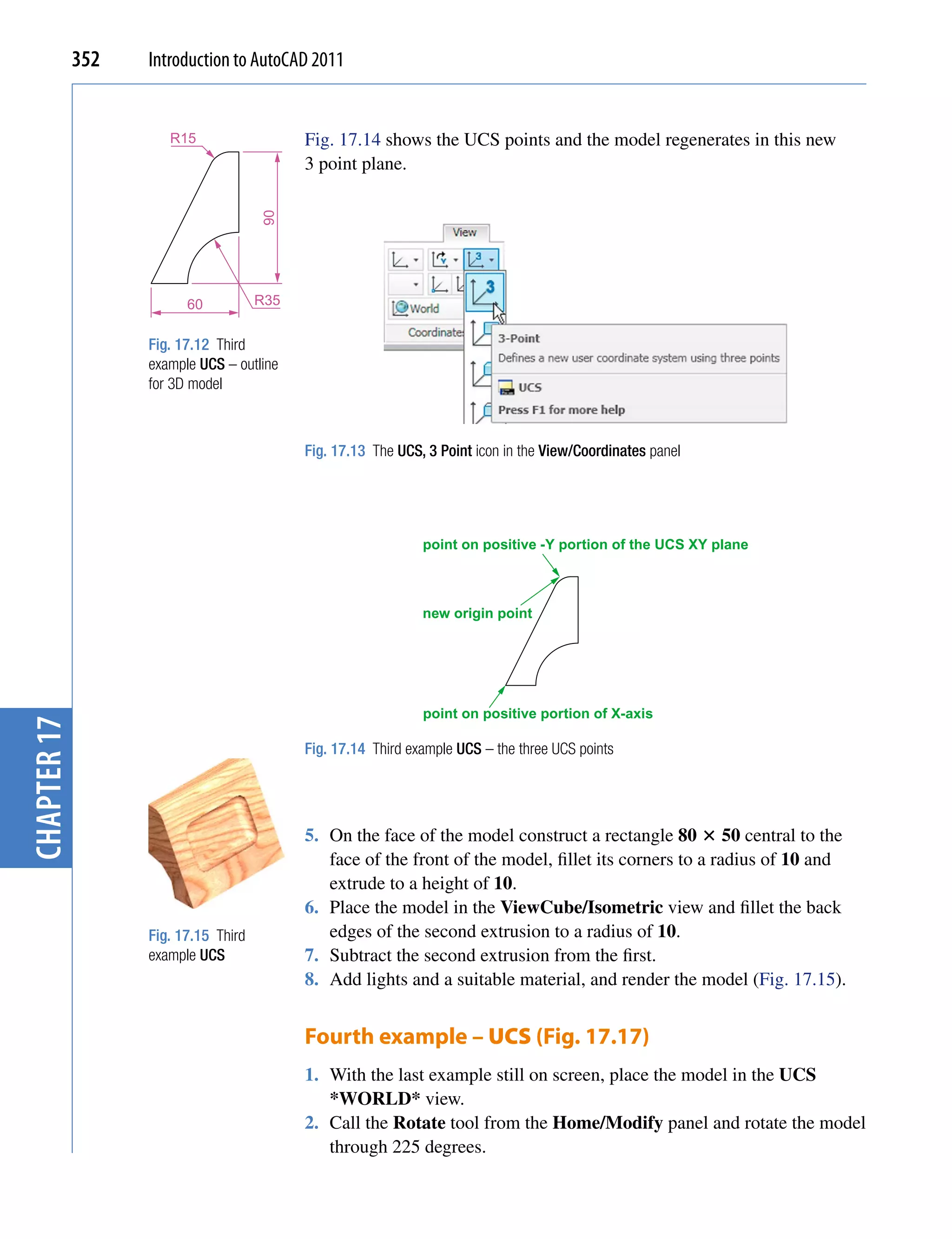
![Three-dimensional space 353
3. Click the X tool icon in the View/Coordinates panel (Fig. 17.16):
Fig. 17.16 The UCS X tool in the View/Coordinates panel
Command: _ucs
Current ucs name: *WORLD*
Specify origin of UCS or [Face/NAmed/OBject/
Previous/View/World/X/Y/Z/ZAxis] <World>: _x
Specify rotation angle about X axis
<90>: right-click
Regenerating model
Command:
Fig. 17.17 Fourth
4. Render the model in its new UCS plane (Fig. 17.17).
example
chapter 17
Saving UCS views
If a number of different UCS planes are used in connection with the
construction of a 3D model, each view obtained can be saved to a different
name and recalled when required. To save a UCS plane view in which a
3D model drawing is being constructed enter ucs at the command line:
Current ucs name: *NO NAME*
Specify origin of UCS or [Face/NAmed/OBject/
Previous/View/World/X/Y/Z/ZAxis] <World>:
enter s right-click
Enter name to save current UCS or [?]: enter New
View right-click
Regenerating model
Command:
Click the UCS Settings arrow in the View/Coordinates panel and the
UCS dialog appears. Click the Named UCSs tab of the dialog and the
names of views saved in the drawing appear (Fig. 17.18).](https://image.slidesharecdn.com/introductiontoautocad2011-100614022653-phpapp02/75/Introduction-to-AutoCad-2011-345-2048.jpg)
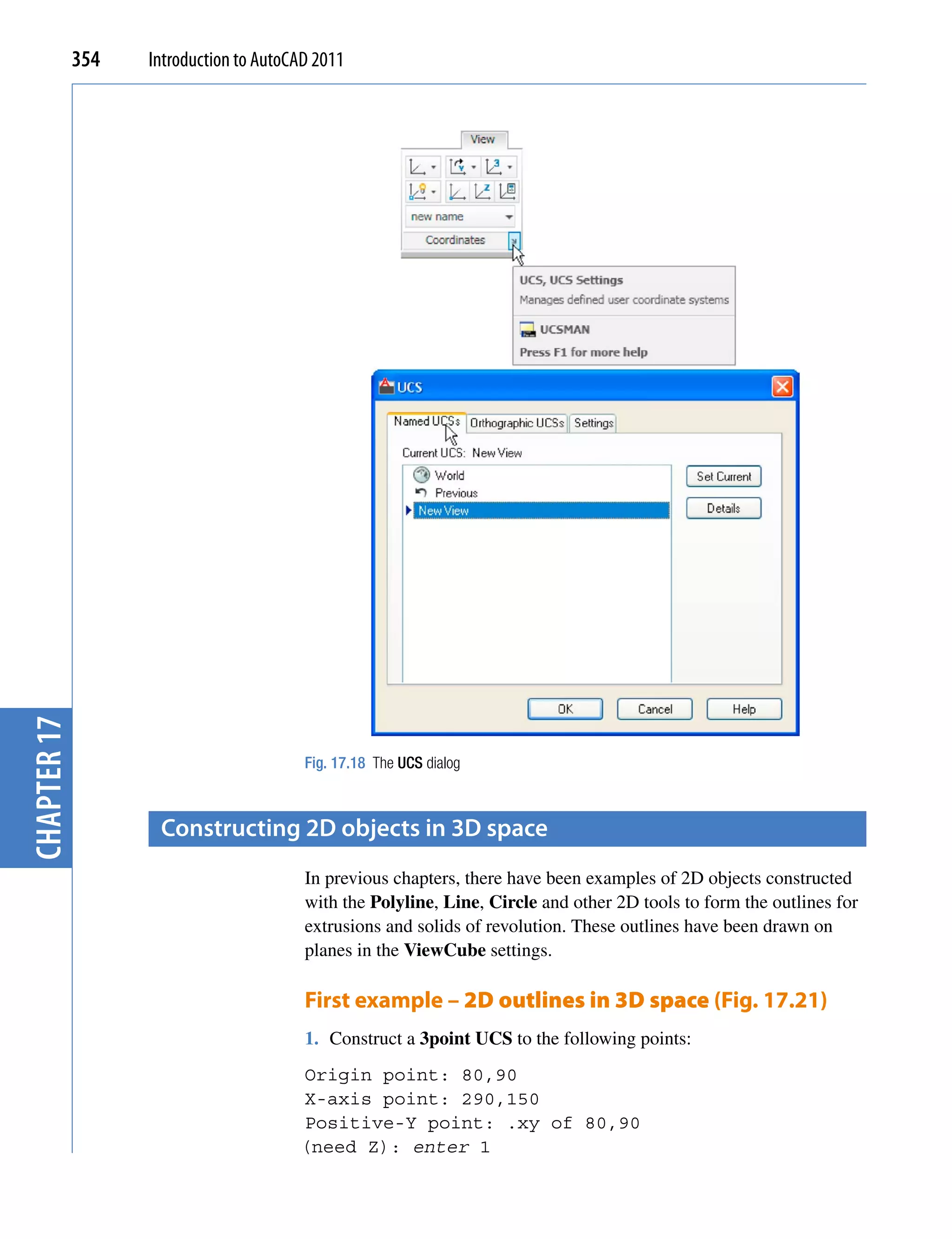
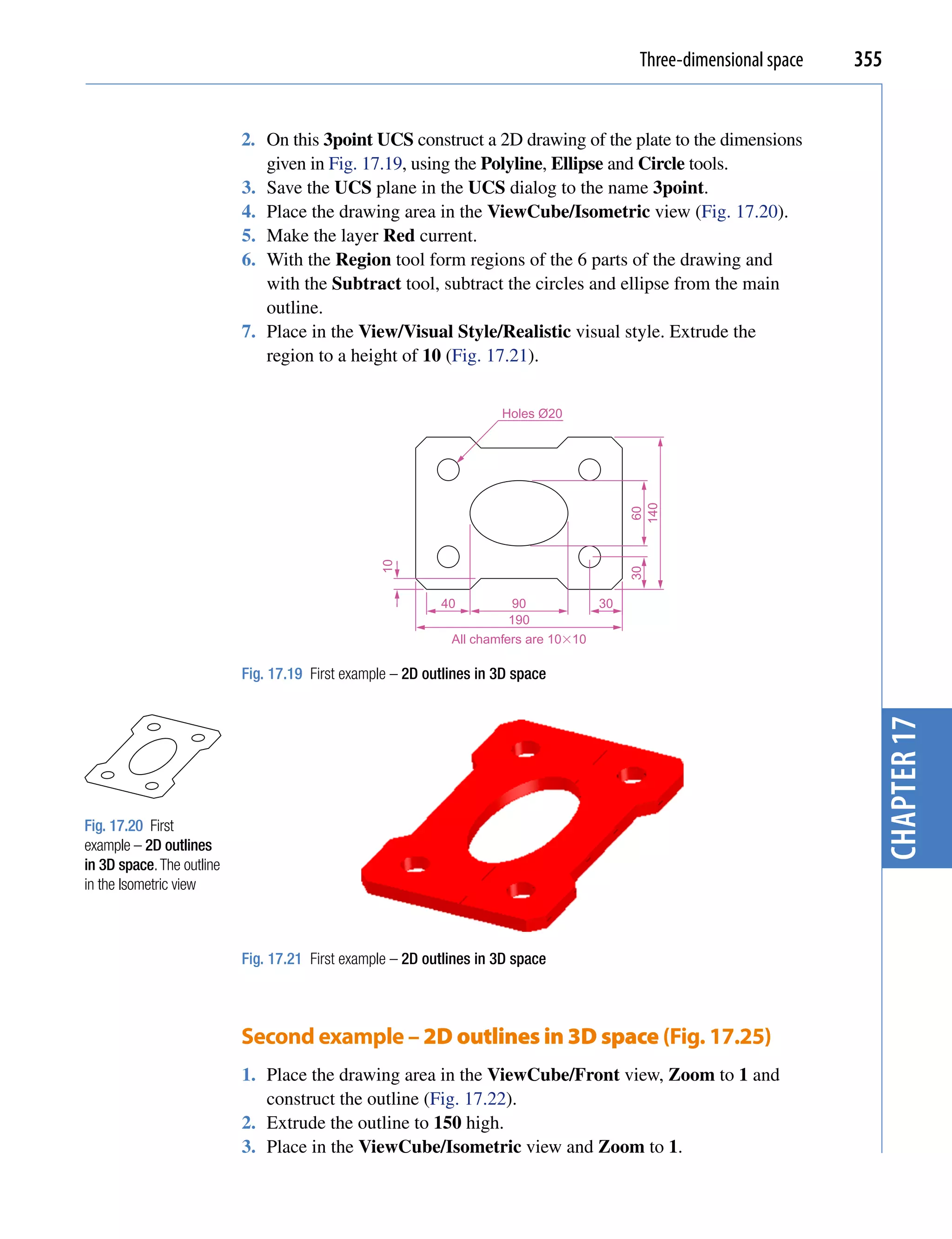
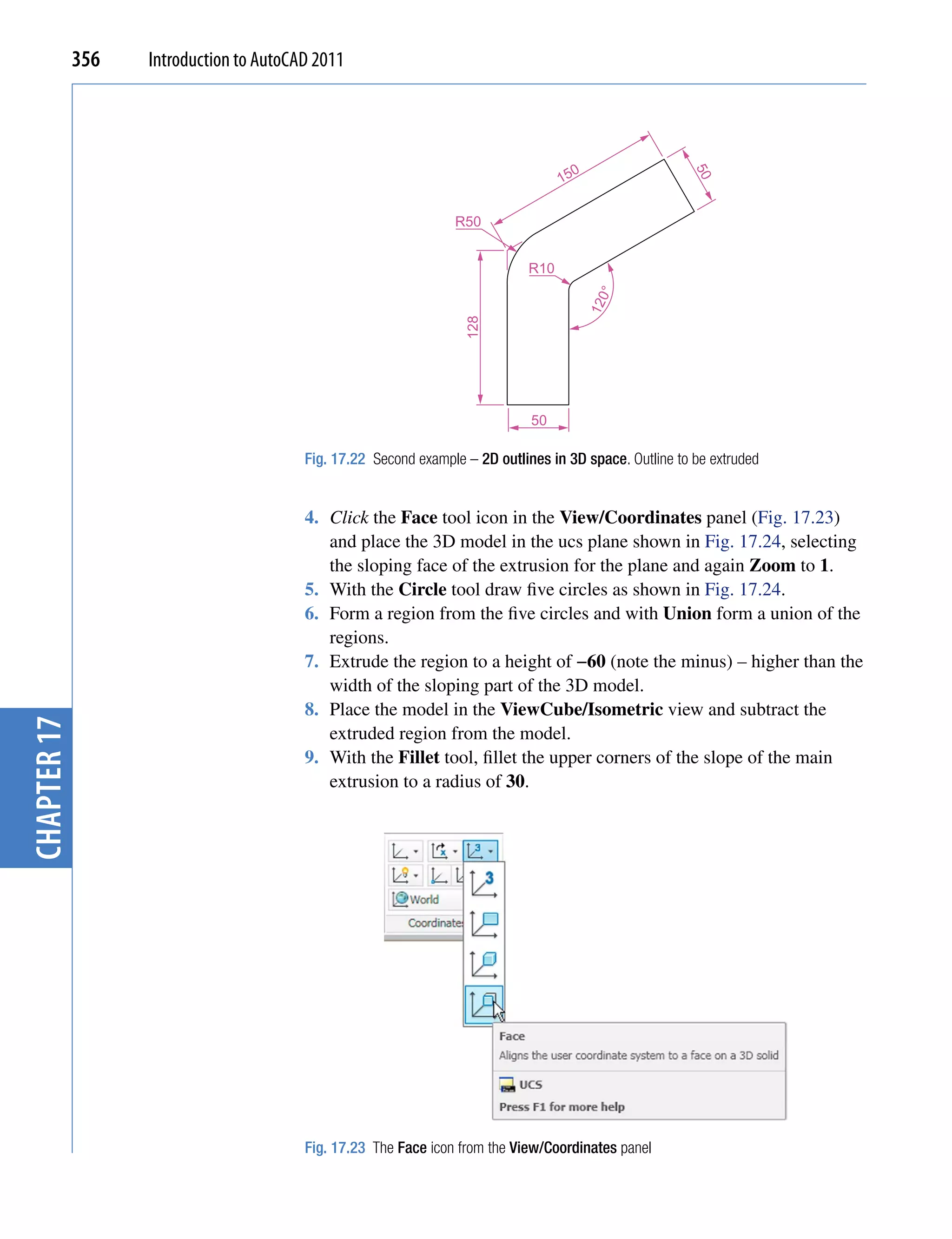
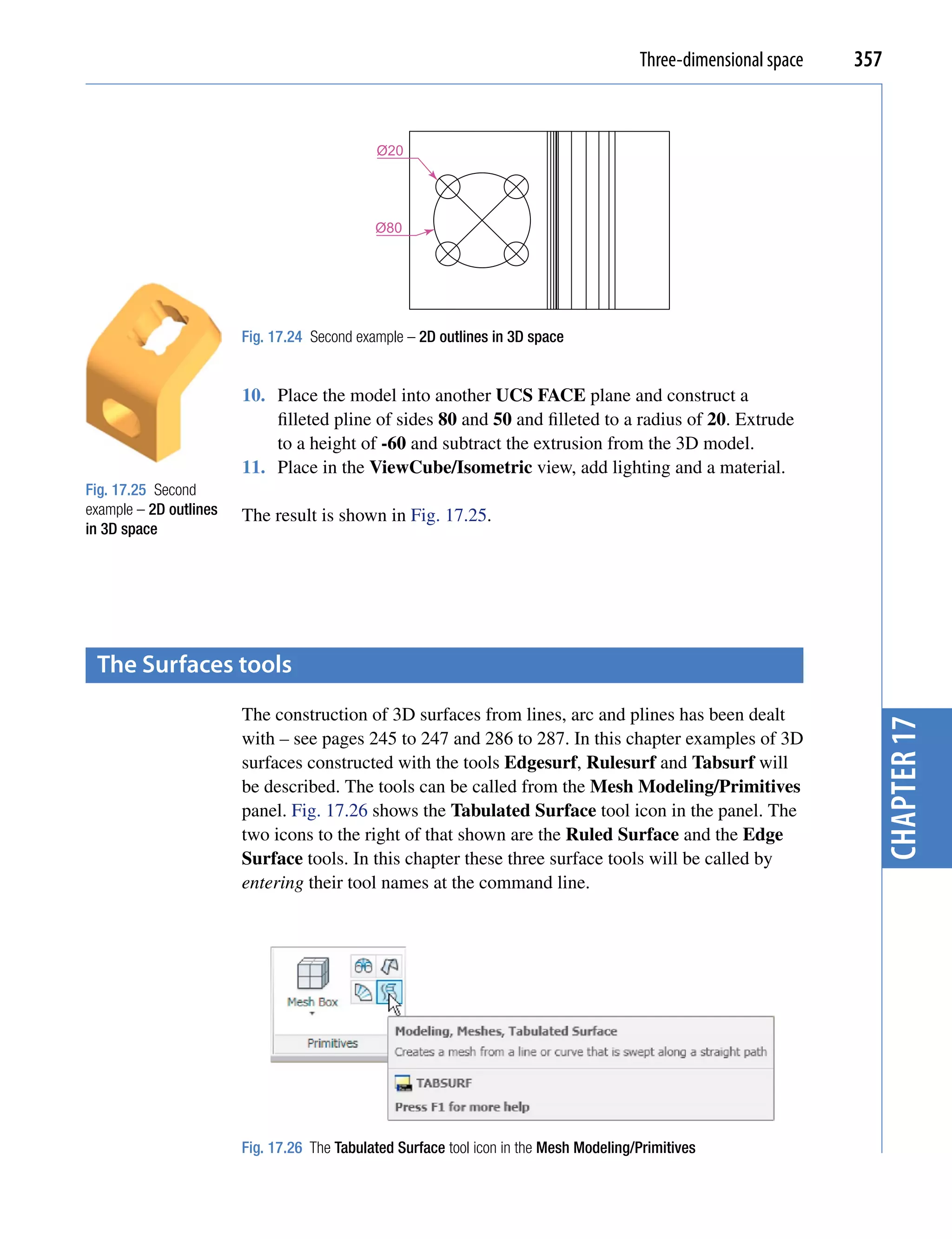
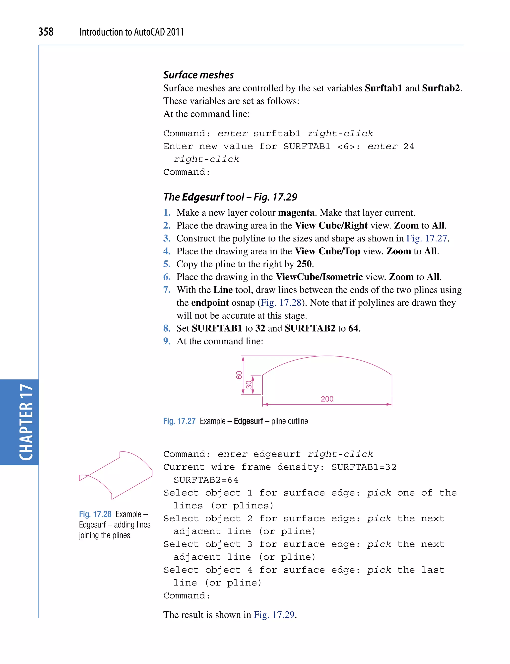
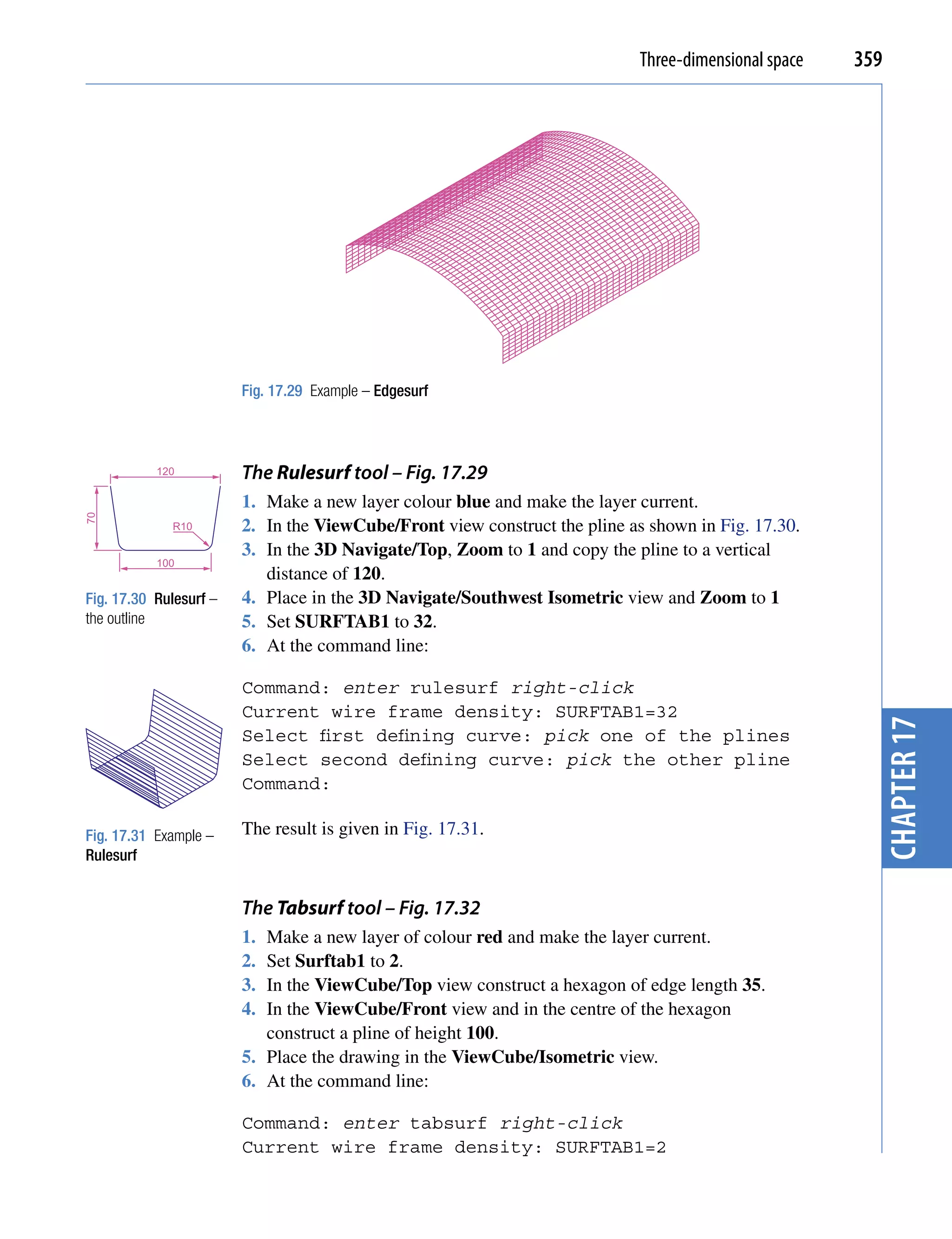
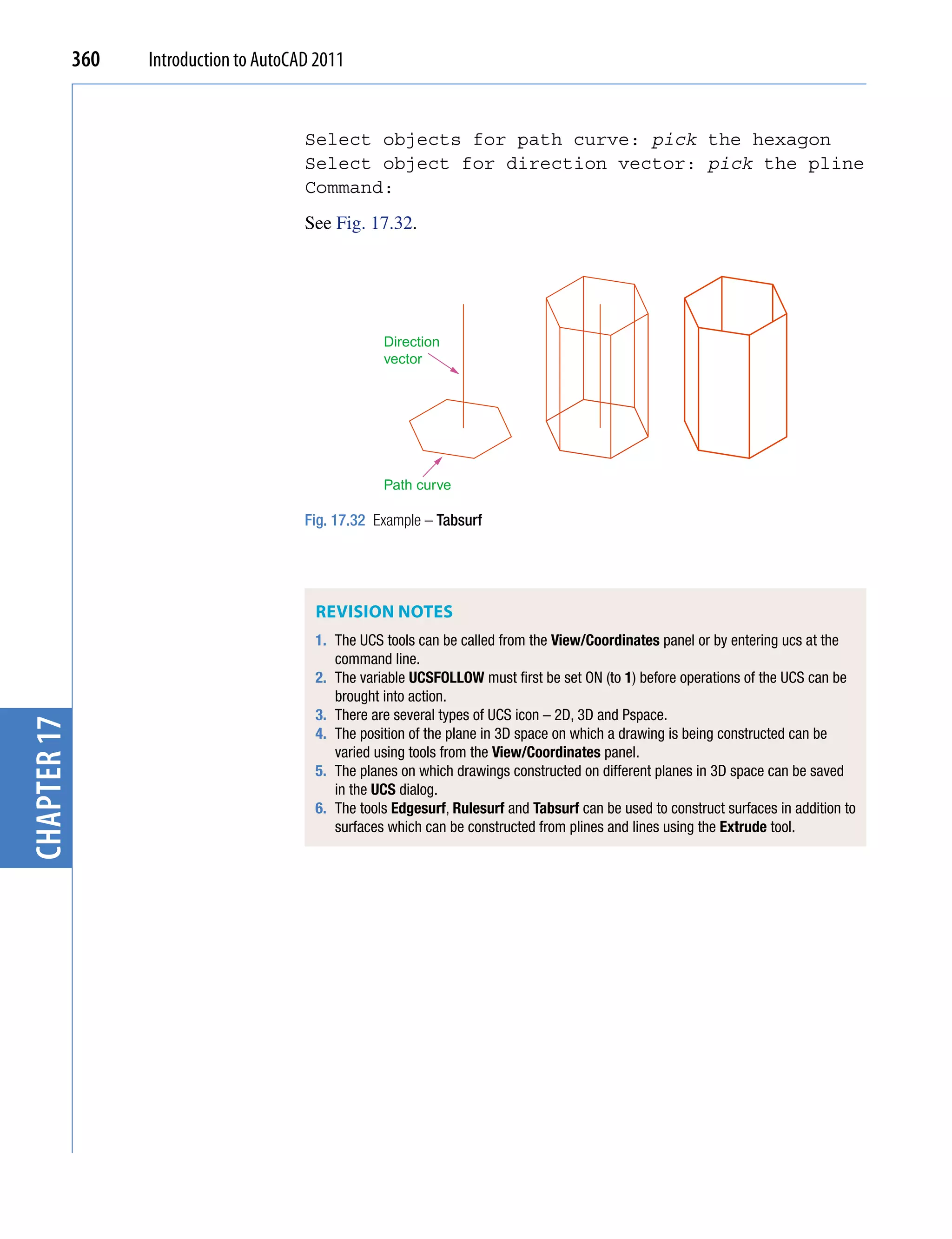
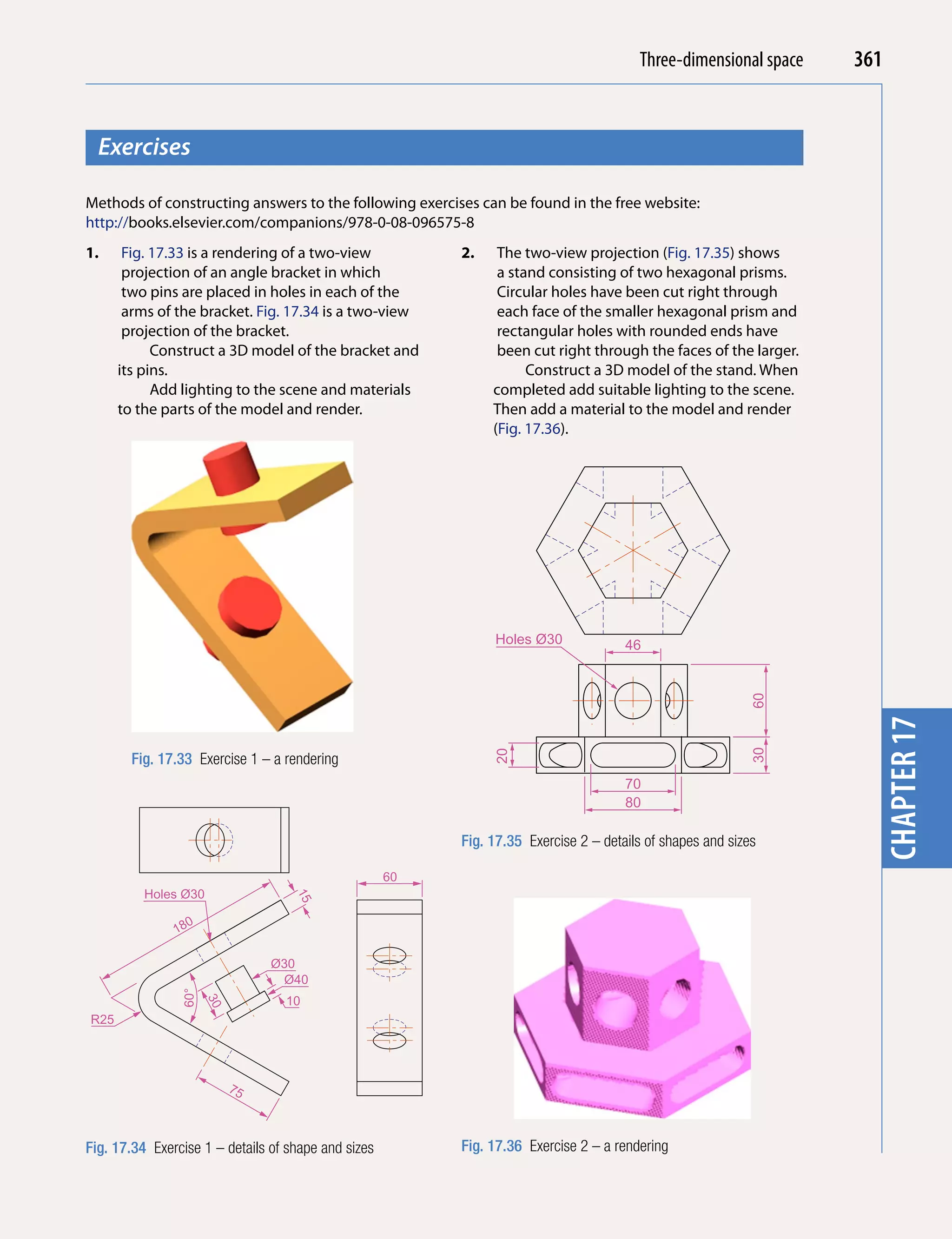
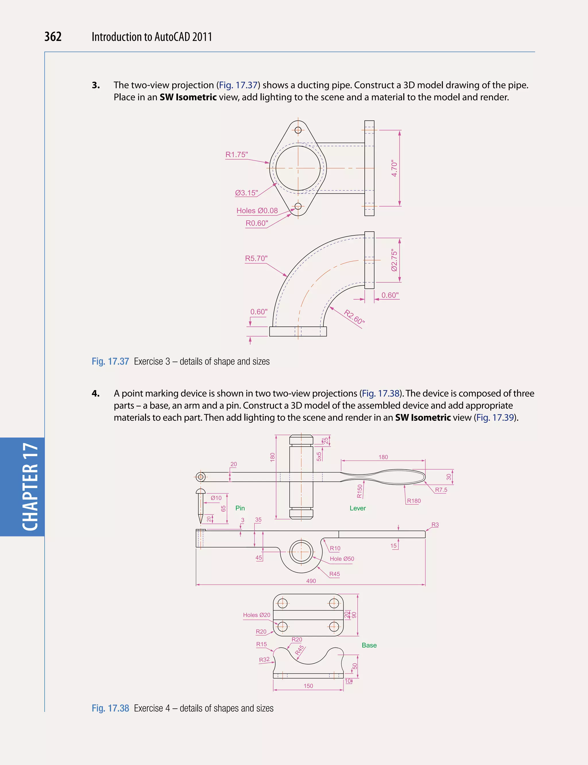
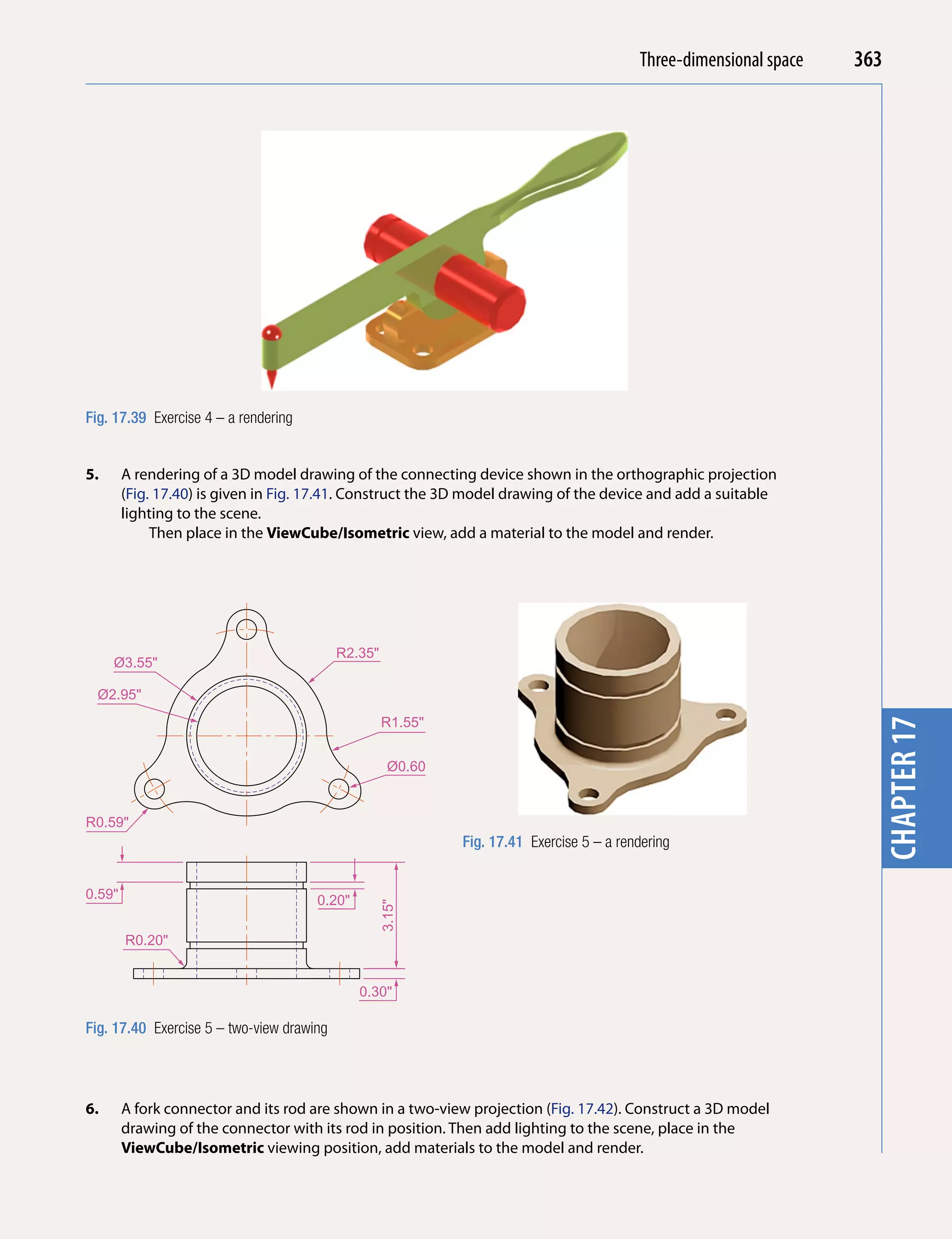
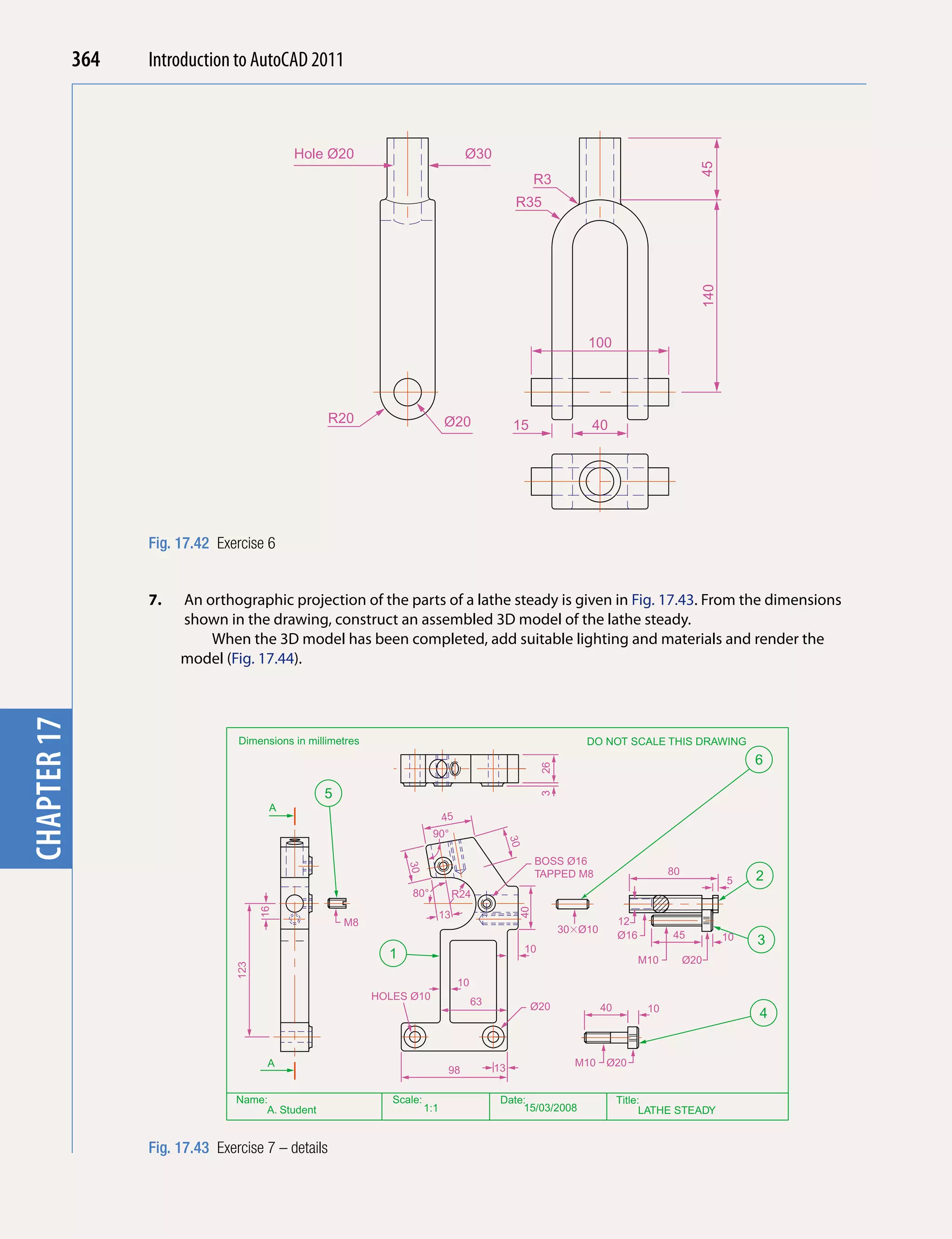
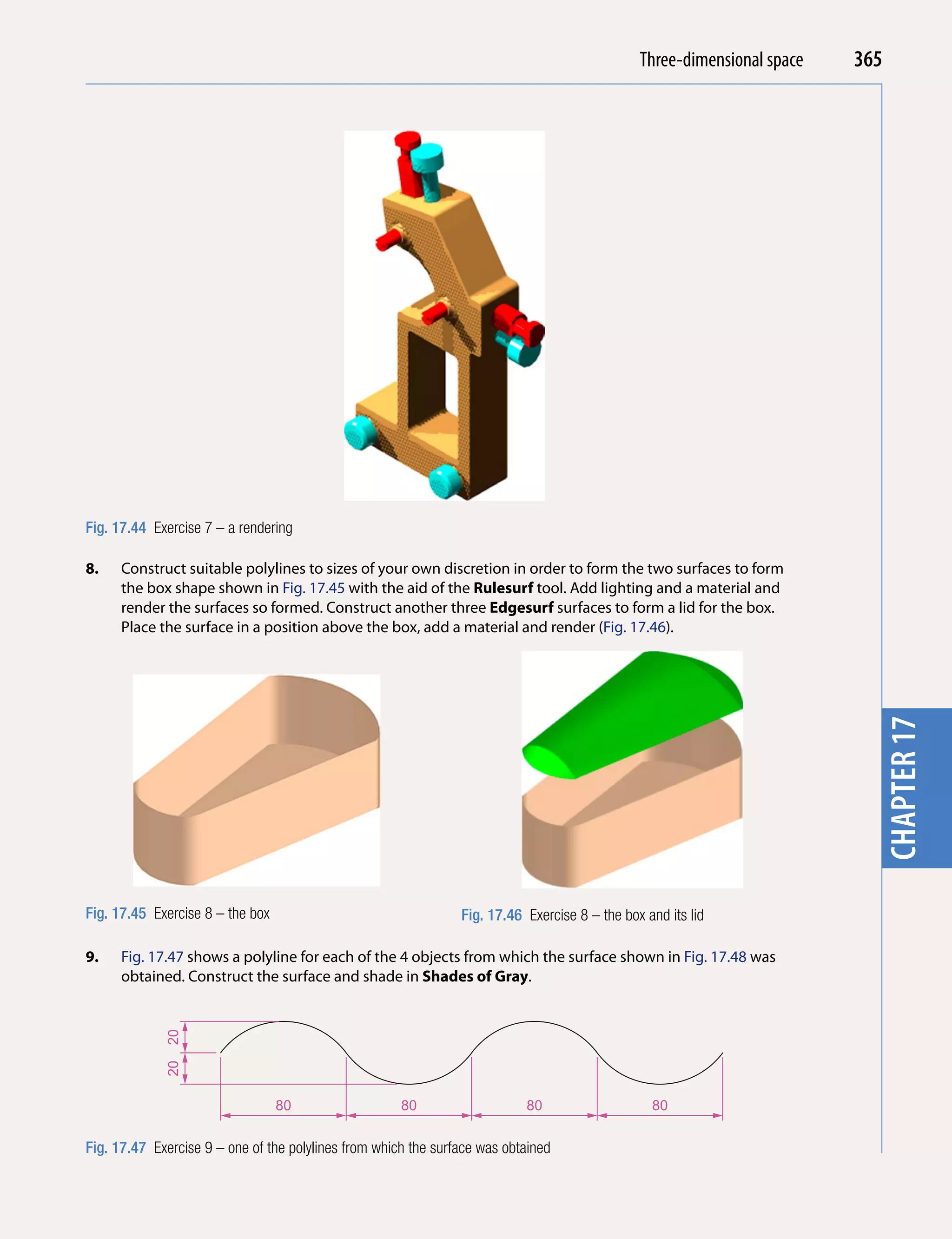
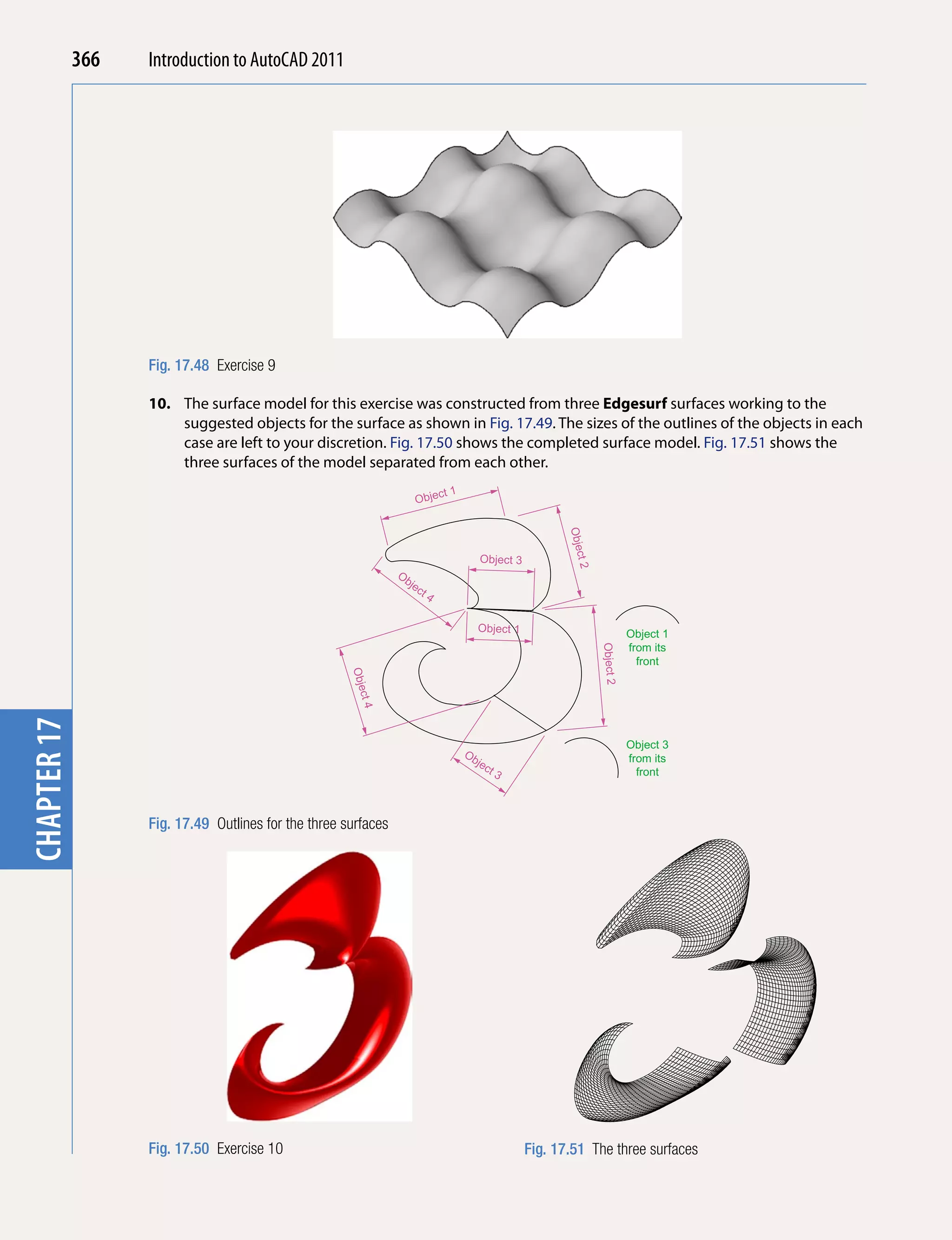
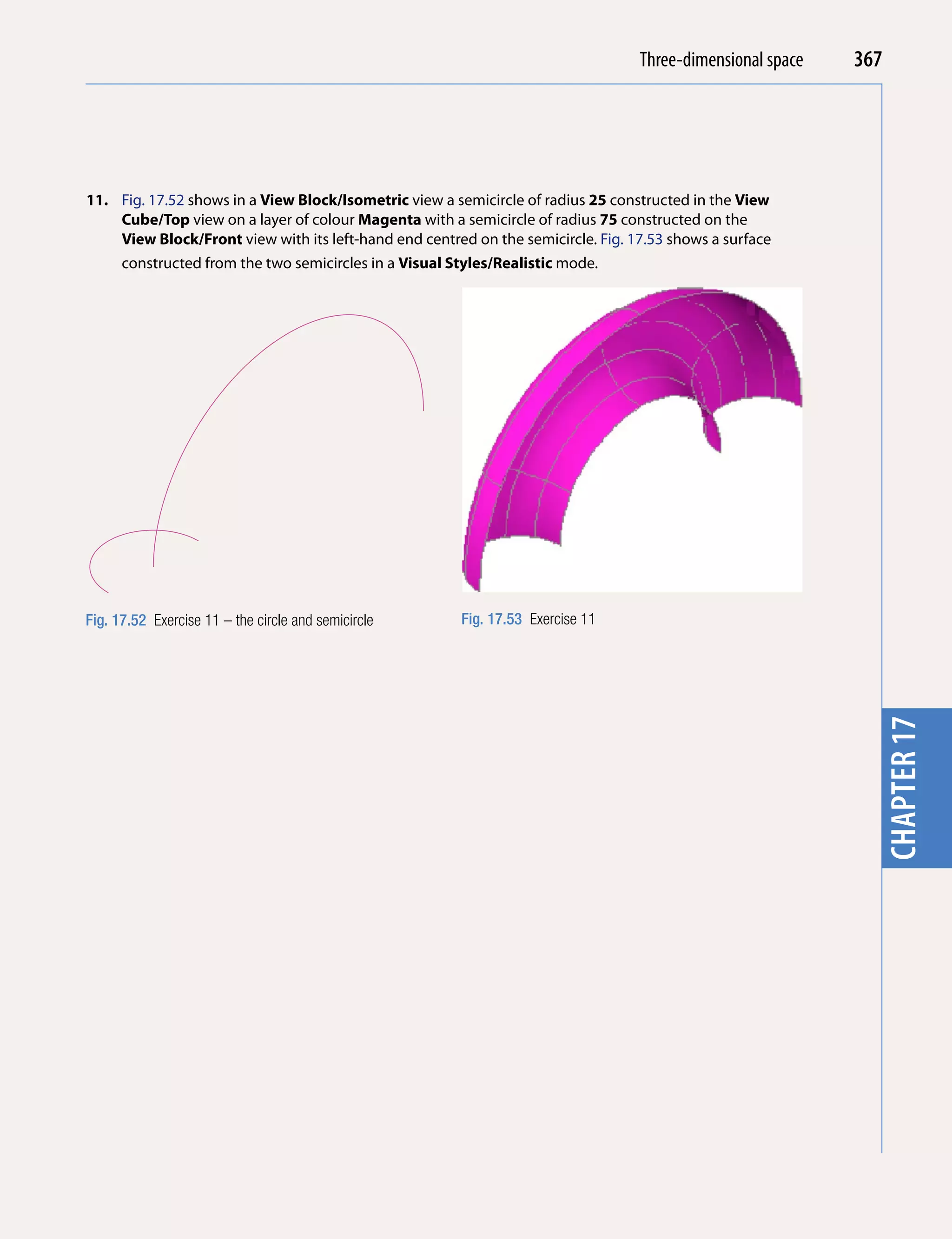
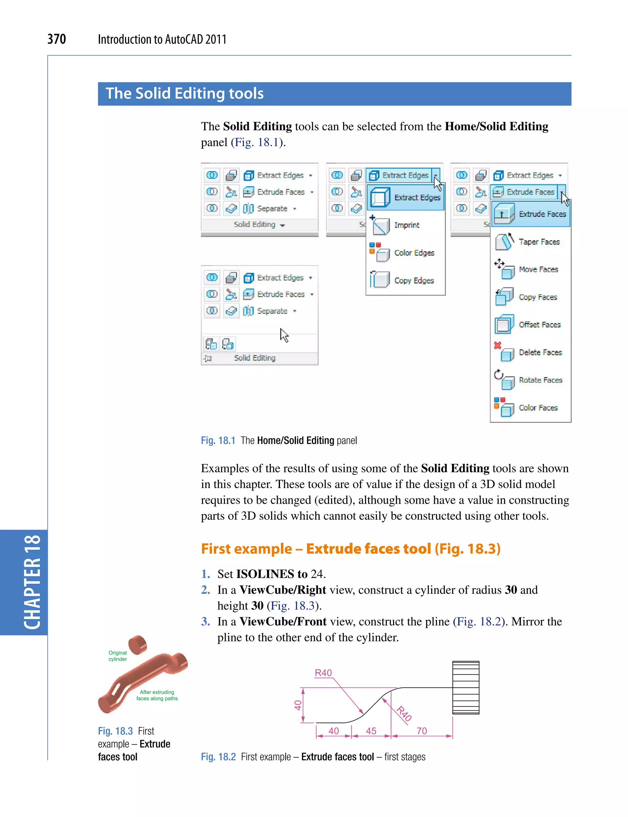
![Editing 3D solid models 371
4. In a ViewCube/Top view, move the pline to lie central to the cylinder.
5. Place the screen in a ViewCube/Isometric view.
6. Click the Extrude faces tool icon in the Home/Solid Editing panel
(Fig. 18.1). The command line shows:
Command: _solidedit
Solids editing automatic checking: SOLIDCHECK=1
Enter a solids editing option [Face/Edge/Body/
Undo/eXit] <eXit>: _face
Enter a face editing option
[Extrude/Move/Rotate/Offset/Taper/Delete/Copy/
coLor/mAterial/Undo/eXit] <eXit>: _extrude
Select faces or [Undo/Remove]: pick the cylinder 2
faces found.
Select faces or [Undo/Remove/ALL]: enter r right-
click
Remove faces or [Undo/Add/ALL]: right-click
Specify height of extrusion or [Path]: enter
p (Path)right-click
Select extrusion path: pick the left-hand path
pline
Solid validation started.
Solid validation completed.
Enter a face editing option [Extrude/Move/Rotate/
Offset/Taper/Delete/Copy/coLor/mAterial/Undo/
eXit] <eXit>: right-click
Command:
7. Repeat the operation using the pline at the other end of the cylinder as a
path.
chapter 18
8. Add lights and a material and render the 3D model (Fig. 18.3).
Note
Path -
Note the prompt line which includes the statement SOLIDCHECK=1.
a pline If the variable SOLIDCHECK is set on (to 1) the prompt lines include
the lines SOLIDCHECK=1, Solid validation started and Solid
Extruded hexagon
of height 1 unit validation completed. If set to 0 these two lines do not show.
Fig. 18.4 Second Second example – Extrude faces tool (Fig. 18.5)
example – Extrude
faces tool – pline for 1. Construct a hexagonal extrusion just 1 unit high in the ViewCube/Top.
path 2. Change to the ViewCube/Front and construct the curved pline (Fig. 18.4).](https://image.slidesharecdn.com/introductiontoautocad2011-100614022653-phpapp02/75/Introduction-to-AutoCad-2011-362-2048.jpg)
![372 Introduction to AutoCAD 2011
3. Back in the Top view, move the pline to lie central to the extrusion.
4. Place in the ViewCube/Isometric view and extrude the top face of the
extrusion along the path of the curved pline.
5. Add lighting and a material to the model and render (Fig. 18.5).
Note
This example shows that a face of a 3D solid model can be extruded
along any suitable path curve. If the polygon on which the extrusion had
been based had been turned into a region, no extrusion could have taken
place. The polygon had to be extruded to give a face to a 3D solid.
Third example – Move faces tool (Fig. 18.6)
1. Construct the 3D solid drawing shown in the left-hand drawing of
Fig. 18.6 from three boxes which have been united using the Union tool.
2. Click on the Move faces tool in the Home/Solid Editing panel (see
Fig. 18.1). The command line shows:
Command: _solidedit
[prompts] _face
Enter a face editing option
[prompts]: _move
Select faces or [Undo/Remove]: pick the model face
4 face found.
Select faces or [Undo/Remove/ALL]: right-click
Specify a base point or displacement: pick
Specify a second point of displacement: pick
Fig. 18.5 Second [further prompts]:
chapter 18
example – Extrude
faces tool And the picked face is moved – right-hand drawing of Fig. 18.6.
Before After
Move Faces Move Faces
Fig. 18.6 Third example – Solid, Move faces tool](https://image.slidesharecdn.com/introductiontoautocad2011-100614022653-phpapp02/75/Introduction-to-AutoCad-2011-363-2048.jpg)
![Editing 3D solid models 373
Fourth example – Offset faces (Fig. 18.7)
1. Construct the 3D solid drawing shown in the left-hand drawing of
Fig. 18.7 from a hexagonal extrusion and a cylinder which have been
united using the Union tool.
Original model Upper Face Side Face
Offset Offset
Bottom Face
Offset
Fig. 18.7 Fourth example – Offset faces tool
2. Click on the Offset faces tool icon in the Home/Solid Editing panel
(Fig. 18.1). The command line shows:
Command:_solidedit
[prompts]:_face
[prompts]
chapter 18
[prompts]:_offset
Select faces or [Undo/Remove]: pick the bottom
face of the 3D model 2 faces found.
Select faces or [Undo/Remove/All]: enter r right-
click
Select faces or [Undo/Remove/All]: pick
highlighted faces other than the bottom face 2
faces found, 1 removed
Select faces or [Undo/Remove/All]: right-click
Specify the offset distance: enter 30 right-click
3. Repeat, offsetting the upper face of the cylinder by 50 and the right-
hand face of the lower extrusion by 15.
The results are shown in Fig. 18.9.](https://image.slidesharecdn.com/introductiontoautocad2011-100614022653-phpapp02/75/Introduction-to-AutoCad-2011-364-2048.jpg)
![374 Introduction to AutoCAD 2011
Fifth example – Taper faces tool (Fig. 18.8)
1. Construct the 3D model as in the left-hand drawing of Fig. 18.8. Place
in ViewCube/Isometric view.
Before Taper Faces After Taper Faces
Fig. 18.8 Fifth example – Taper faces tool
2. Call Taper faces. The command line shows:
Command:_solidedit
[prompts]:_face
[prompts]
[prompts]:_taper
Select faces or [Undo/Remove]: pick the upper face
of the base 2 faces found.
Select faces or [Undo/Remove/All]: enter r right-
click
chapter 18
Select faces or [Undo/Remove/All]: pick
highlighted faces other than the upper face 2
faces found, 1 removed
Select faces or [Undo/Remove/All]: right-click
Specify the base point: pick a point on left-hand
edge of the face
Specify another point along the axis of tapering:
pick a point on the right-hand edge of
the face
Specify the taper angle: enter 10 right-click
And the selected face tapers as indicated in the right-hand drawing of
Fig. 18.8.](https://image.slidesharecdn.com/introductiontoautocad2011-100614022653-phpapp02/75/Introduction-to-AutoCad-2011-365-2048.jpg)
![Editing 3D solid models 375
Sixth example – Copy faces tool (Fig. 18.10)
1. Construct a 3D model to the sizes as given in Fig. 18.9.
180 R20
130
90
R20
R15 Ø50
All offsets are 5 Ø60
R50
20
5
250
Fig. 18.9 Sixth example – Copy Faces tool – details of the 3D solid model
2. Click on the Copy faces tool in the Home/Solid Editing panel
(Fig. 18.1). The command line shows:
Command:_solidedit
[prompts]:_face
[prompts]
[prompts]:_copy
Select faces or [Undo/Remove]: pick the upper face
chapter 18
of the solid model 2 faces found.
Select faces or [Undo/Remove/All]: enter r right-
click
Select faces or [Undo/Remove/All]: pick highlighted
face not to be copied 2 faces found, 1 removed
Select faces or [Undo/Remove/All]: right-click
Specify a base point or displacement: pick
anywhere on the highlighted face
Specify a second point of displacement: pick
a point some 50 units above the face
3. Add lights and a material to the 3D model and its copied face and
render (Fig. 18.10).](https://image.slidesharecdn.com/introductiontoautocad2011-100614022653-phpapp02/75/Introduction-to-AutoCad-2011-366-2048.jpg)
![376 Introduction to AutoCAD 2011
Before Copy Faces After Copy Faces
Fig. 18.10 Sixth example – Copy faces tool
Seventh example – Color faces tool (Fig. 18.12)
1. Construct a 3D model of the wheel to the sizes as shown in
Fig. 18.11.
5
10
R5
50
Ø220
R90 Ø210
R70 Ø200
chapter 18
Ø40
R35
Fig. 18.11 Seventh example – Color faces tool – details of the 3D model
2. Click the Color faces tool icon in the Home/Solid Editing panel
(Fig. 18.1). The command line shows:
Command:_solidedit
[prompts]:_face](https://image.slidesharecdn.com/introductiontoautocad2011-100614022653-phpapp02/75/Introduction-to-AutoCad-2011-367-2048.jpg)
![Editing 3D solid models 377
[prompts]
[prompts]:_color
Select faces or [Undo/Remove]: pick the inner face
of the wheel 2 faces found
Select faces or [Undo/Remove/All]: enter r right-
click
Select faces or [Undo/Remove/All]: pick
highlighted faces other than the required face 2
faces found, 1 removed
Enter new color <ByLayer>: enter 1 (which is red)
right-click
3. Add lights and a material to the edited 3D model and render
(Fig. 18.12).
Fig. 18.12 Seventh example – Color faces tool
examples of more 3D models chapter 18
The following 3D models can be constructed in the 3d acadiso.dwt screen.
The descriptions of the stages needed to construct them have been reduced
from those given in earlier pages, in the hope that readers have already
acquired a reasonable skill in the construction of such drawings.
First example (Fig. 18.14)
1. Front view. Construct the three extrusions for the back panel and the
two extruding panels to the details given in Fig. 18.13.](https://image.slidesharecdn.com/introductiontoautocad2011-100614022653-phpapp02/75/Introduction-to-AutoCad-2011-368-2048.jpg)
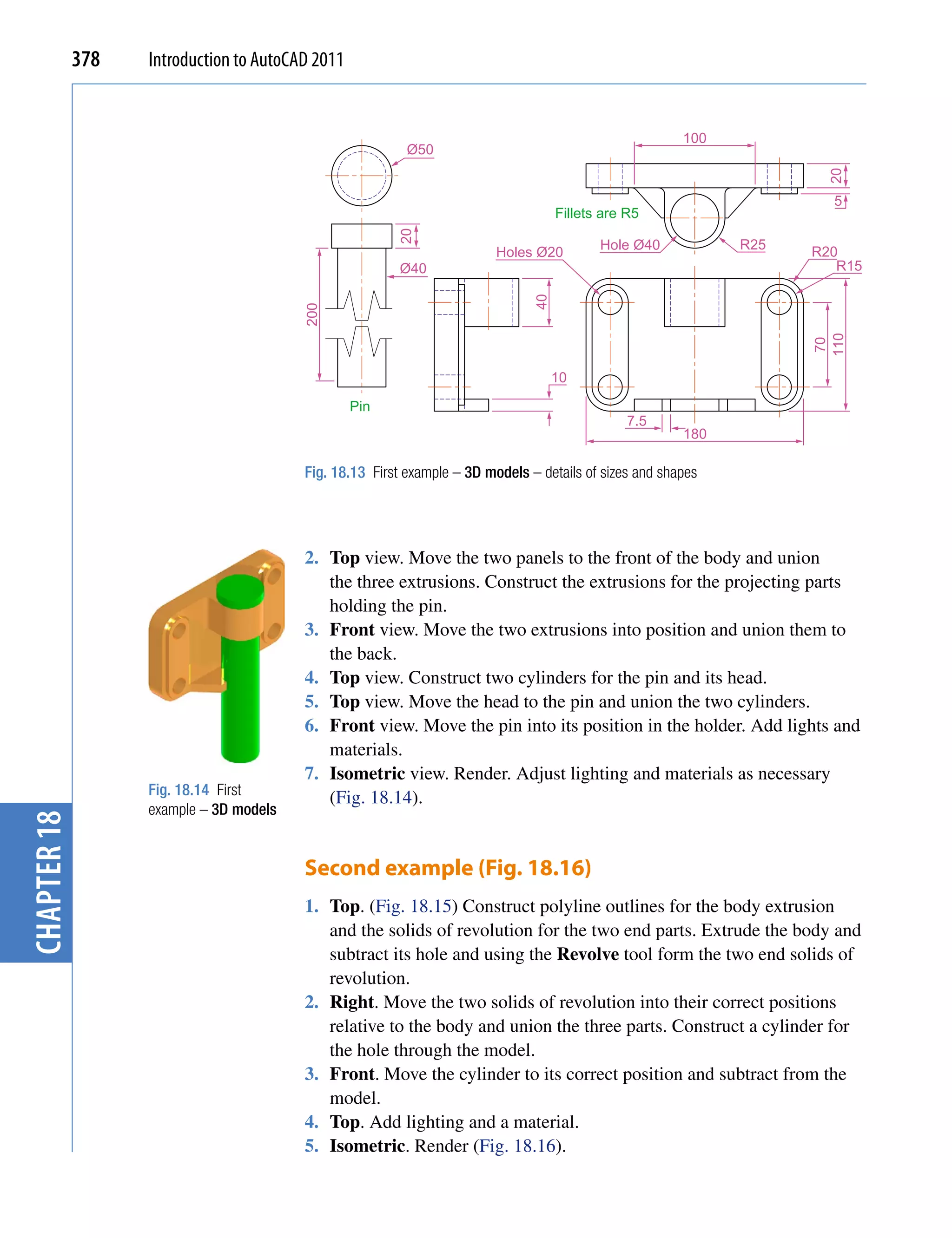
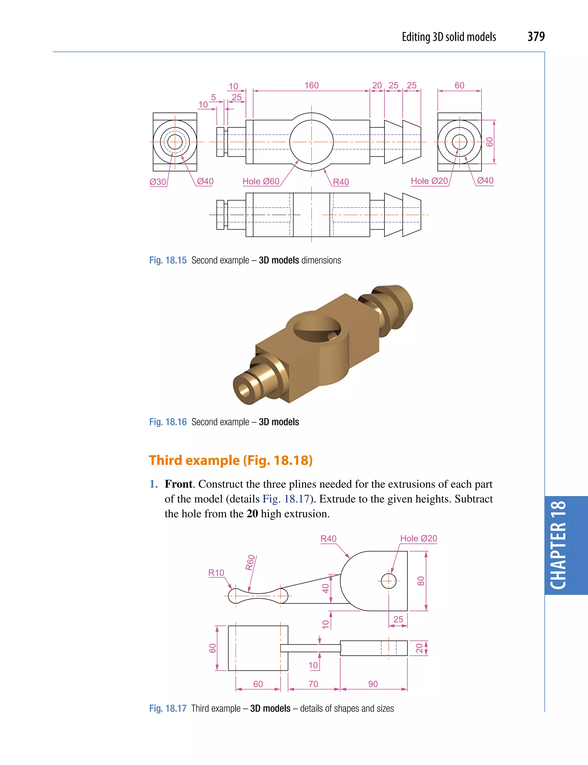
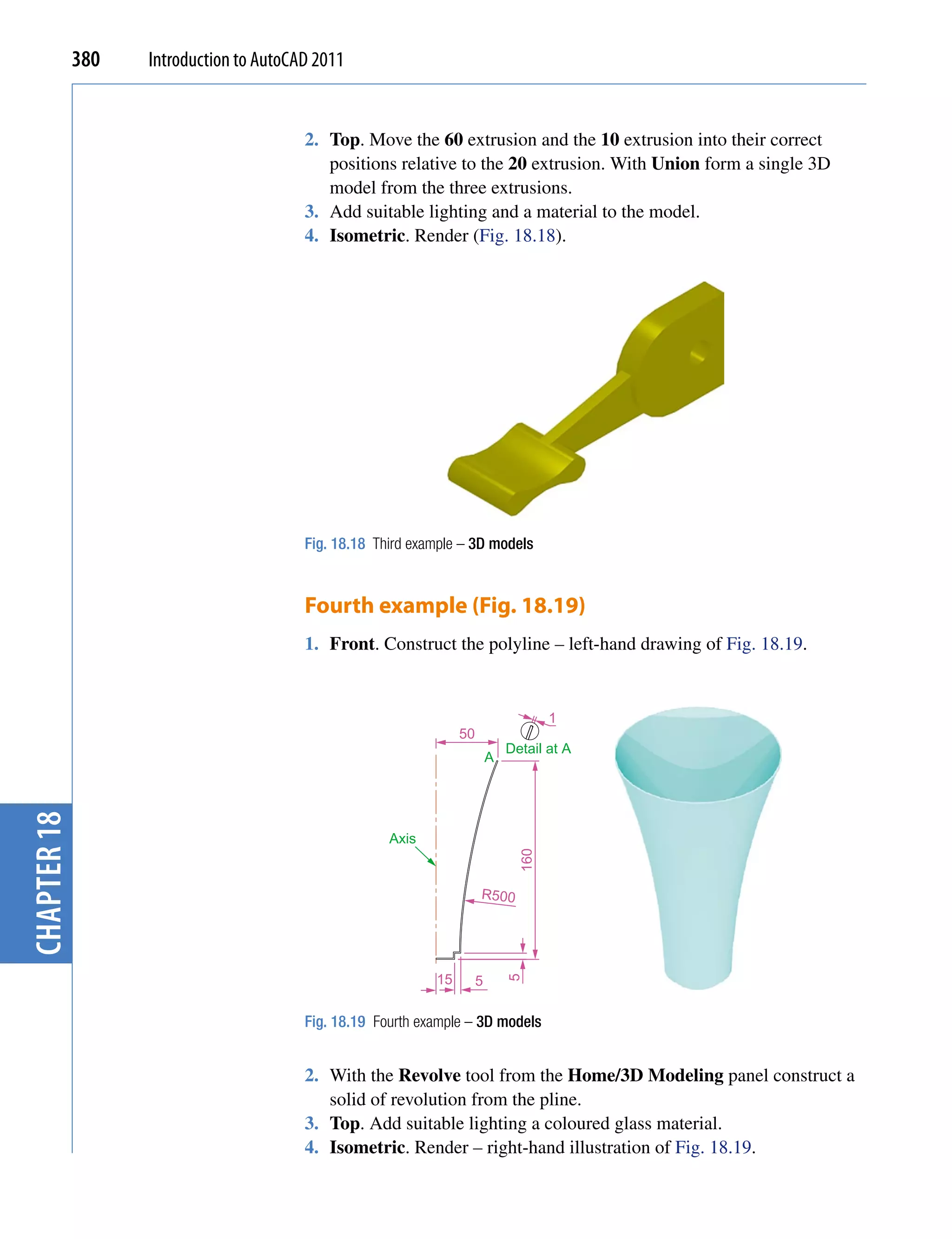
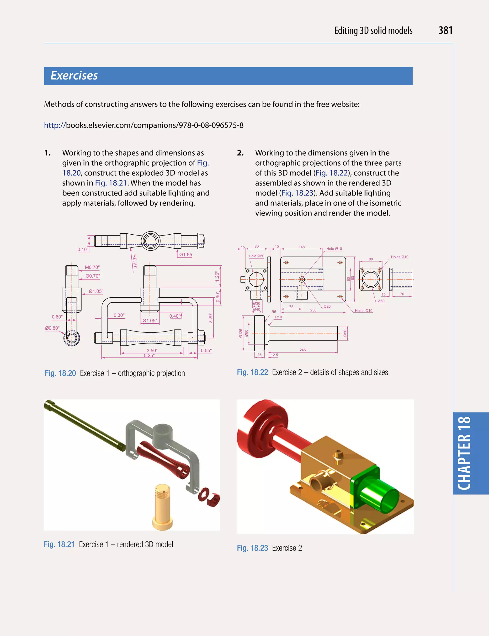
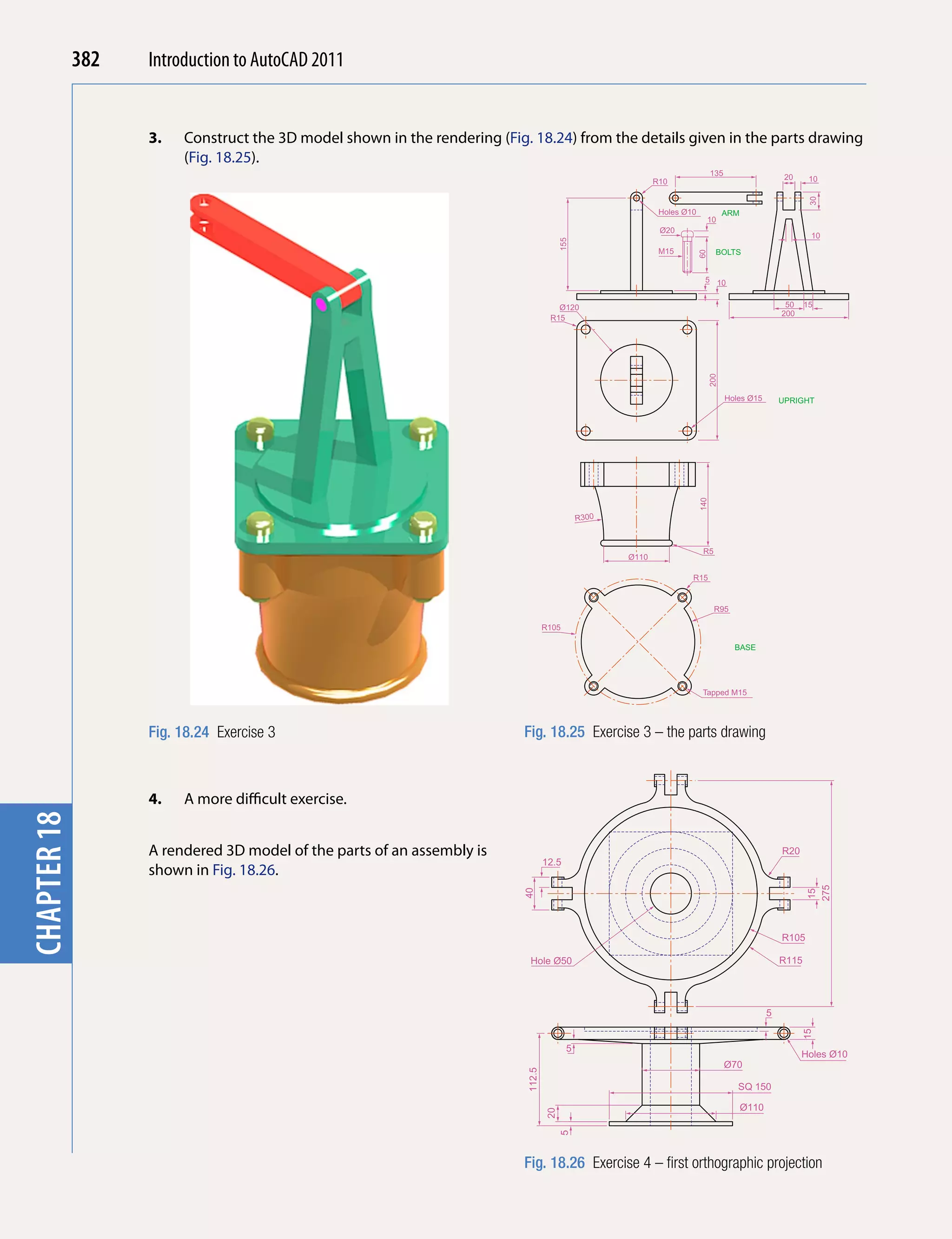
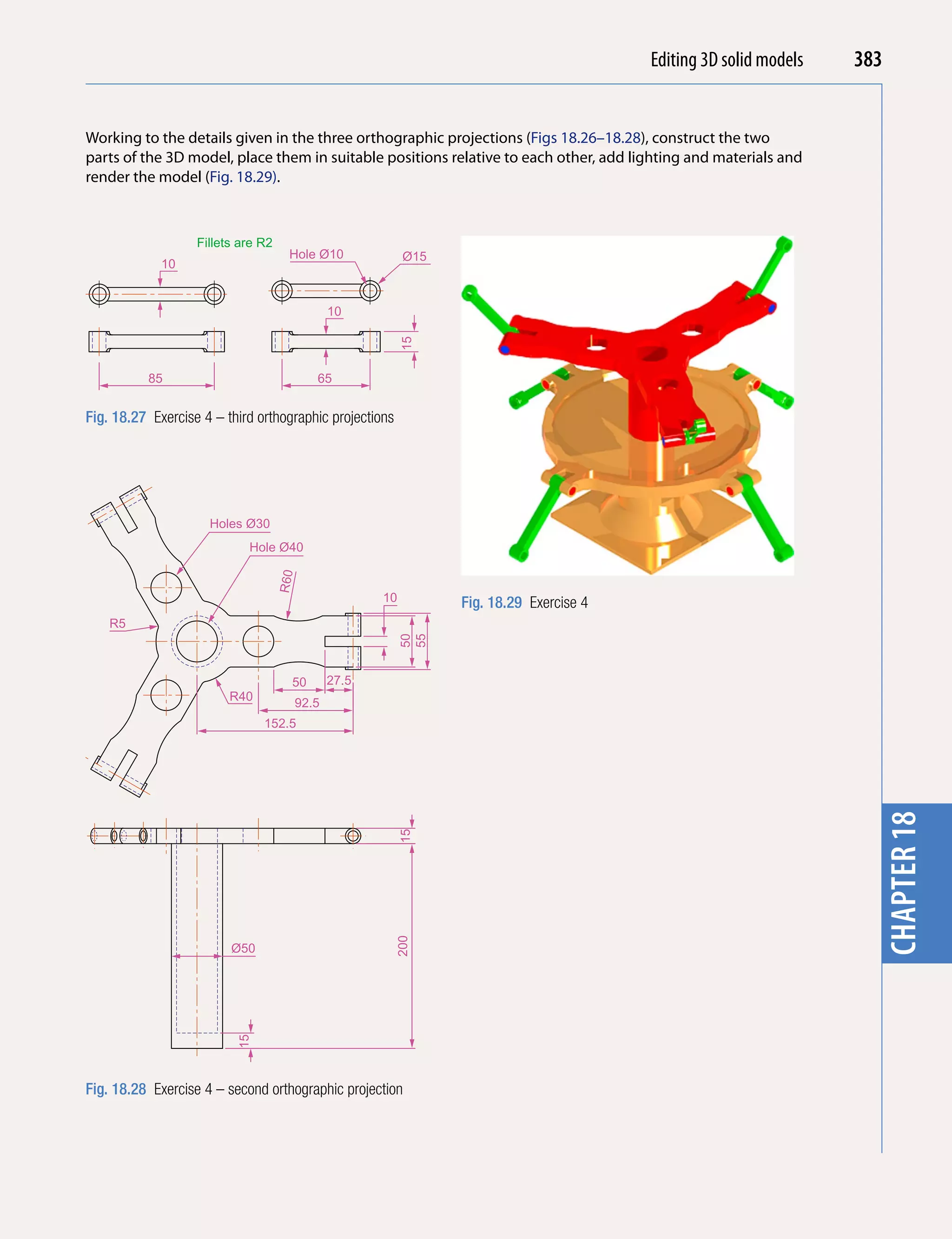
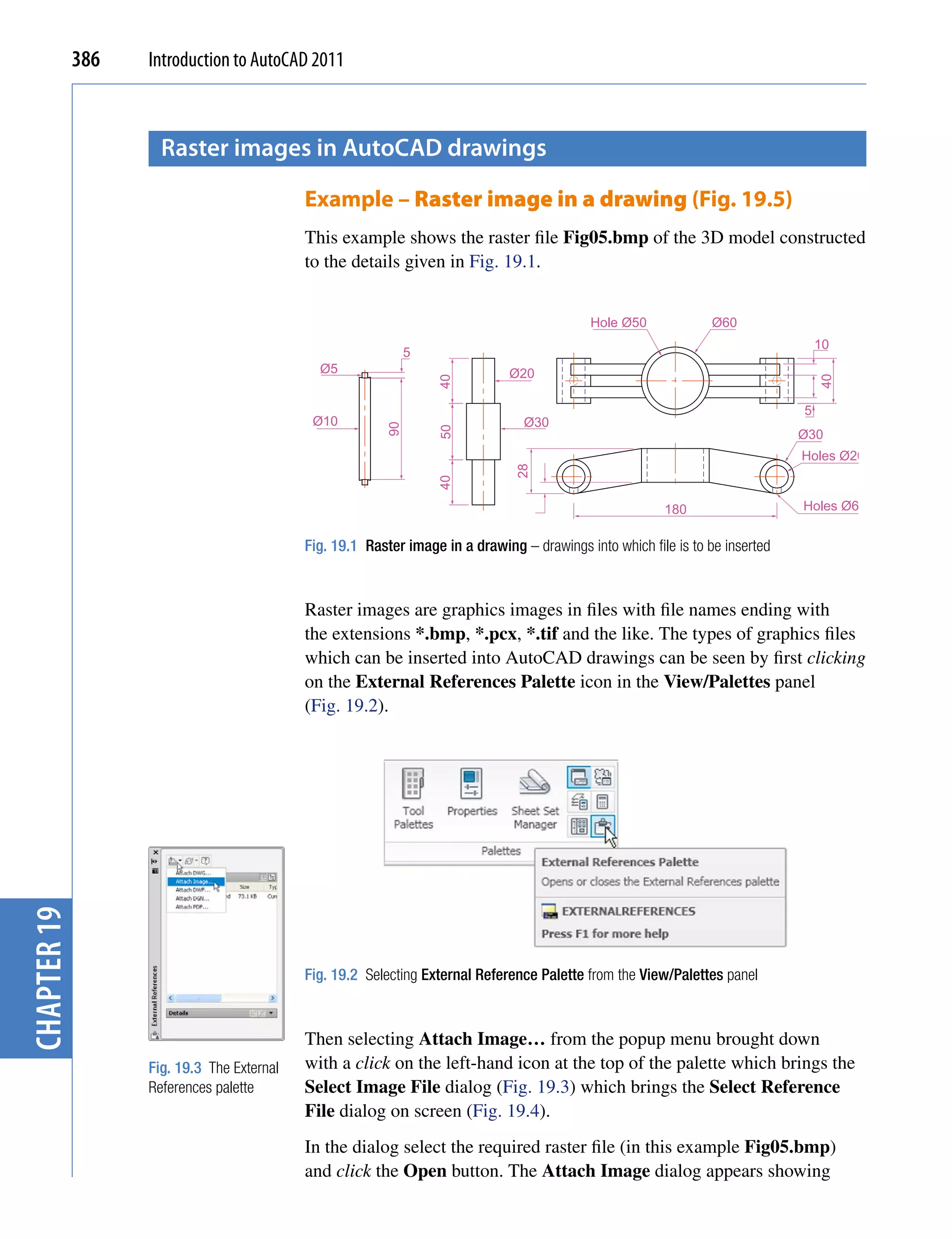
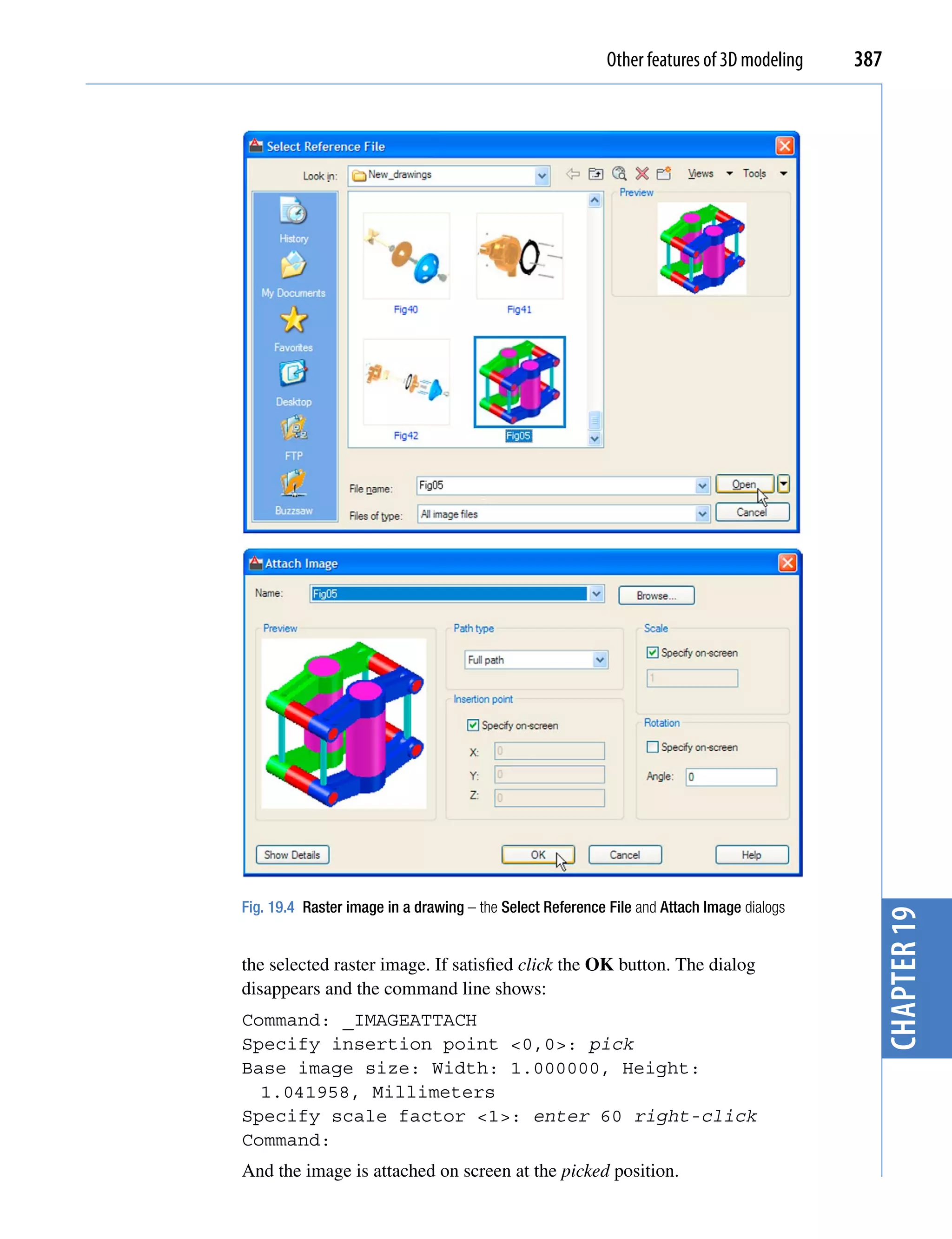
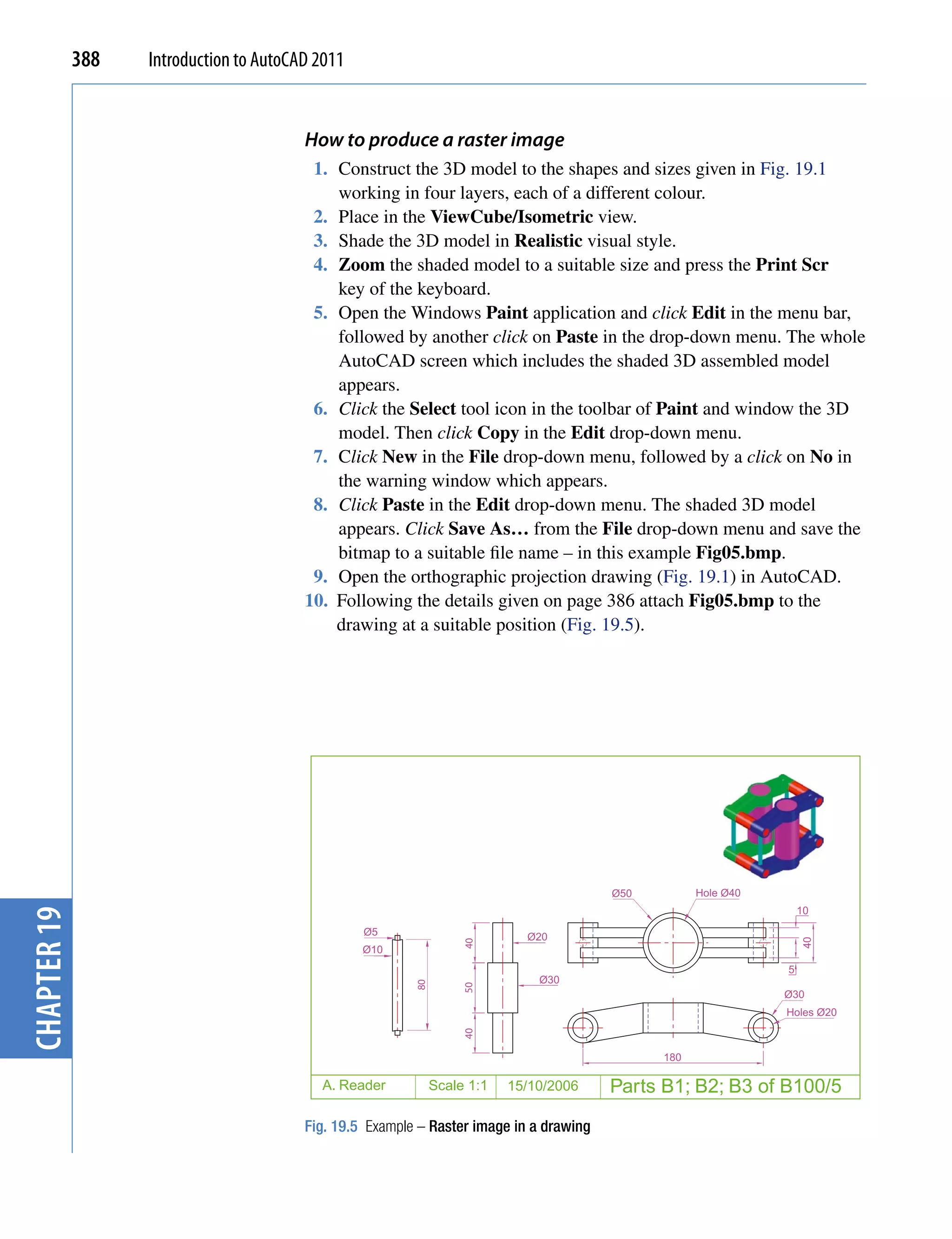
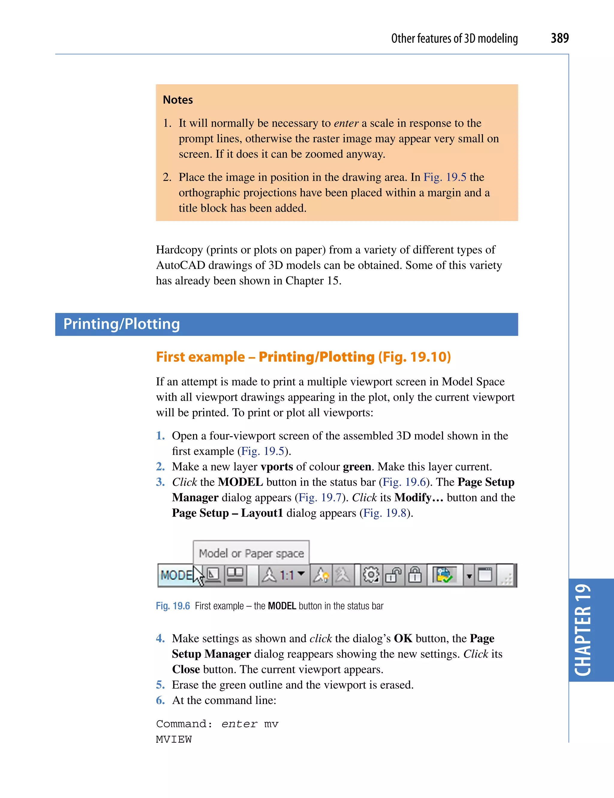
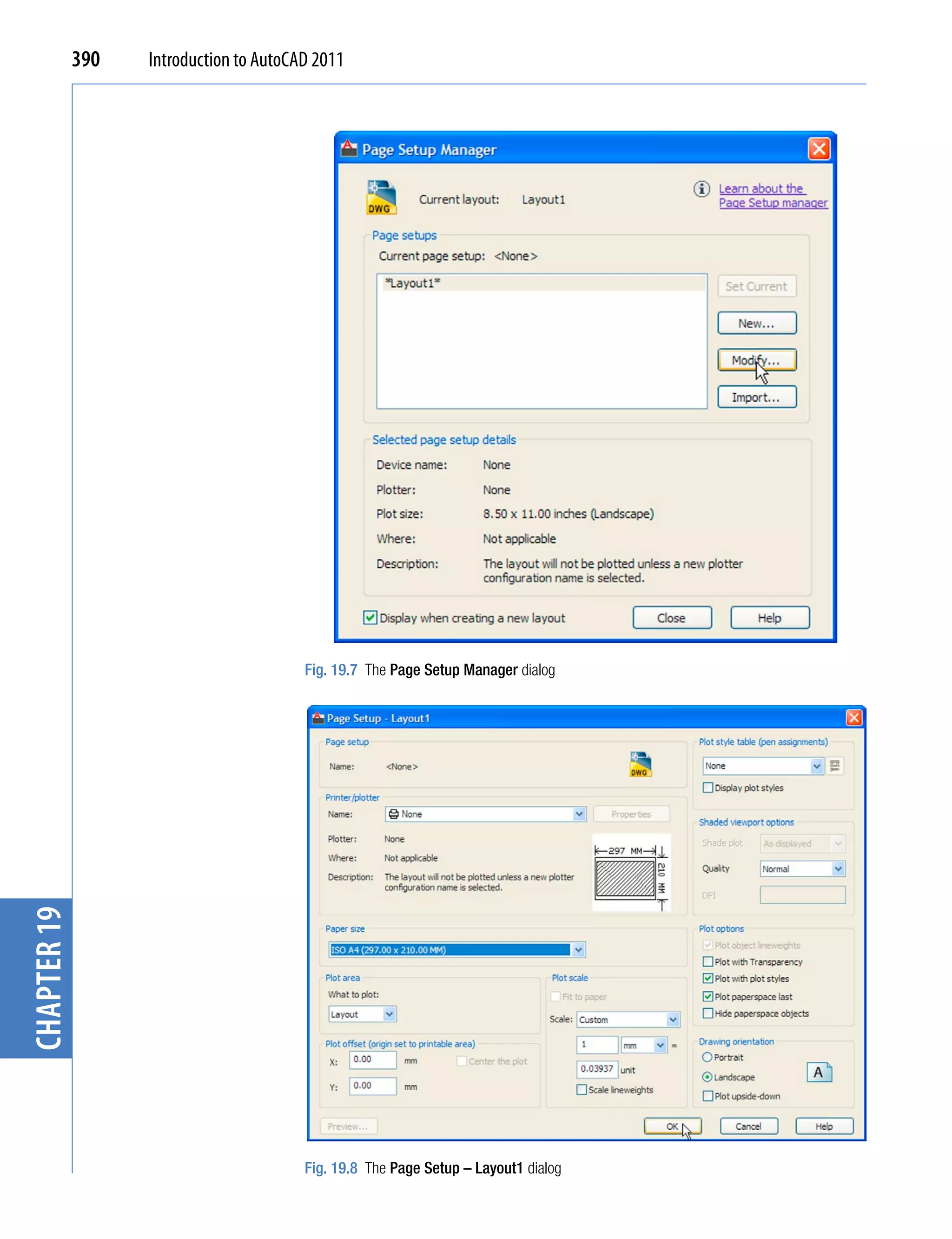
![Other features of 3D modeling 391
Specify corner of viewport or
[ON/OFF/Fit/Shadeplot/Lock/Object/Polygonal/
Restore/LAyer/2/3/4] <Fit>: enter r right-click
Enter viewport configuration name or [?]
<*Active>: right-click
Specify first corner or [Fit] <Fit>: right-
click
Command:
7. Turn layer vports off.
8. Click the PAPER button (note it changes from MODEL) and the
current viewport changes to a model view. In each viewport in turn
change the settings from the 3D Navigation drop-down to Front,
Top, Right and SW isometric. Click the MODEL button. It changes
to PAPER and the screen reverts to Pspace.
9. Click the Plot tool icon in the Quick Access bar (Fig. 19.9). A Plot
dialog appears.
Fig. 19.9 The Plot tool icon in the Quick Access toolbar
10. Check in the dialog that the settings for the printer/plotter is correct
and the paper size is also correct.
11. Click the Preview button. The full preview of the plot appears
(Fig. 19.10). chapter 19
12. Right-click anywhere in the drawing and click on Plot in the right-
click menu which then appears.
13. The drawing plots (or prints).
Second example – Printing/Plotting (Fig. 19.11)
1. Open the orthographic drawing with its raster image (Fig. 19.5).
2. While still in Model Space click the Plot tool icon. The Plot dialog
appears. Check that the required printer/plotter and paper size have
been chosen.
3. Click the Preview button.](https://image.slidesharecdn.com/introductiontoautocad2011-100614022653-phpapp02/75/Introduction-to-AutoCad-2011-381-2048.jpg)
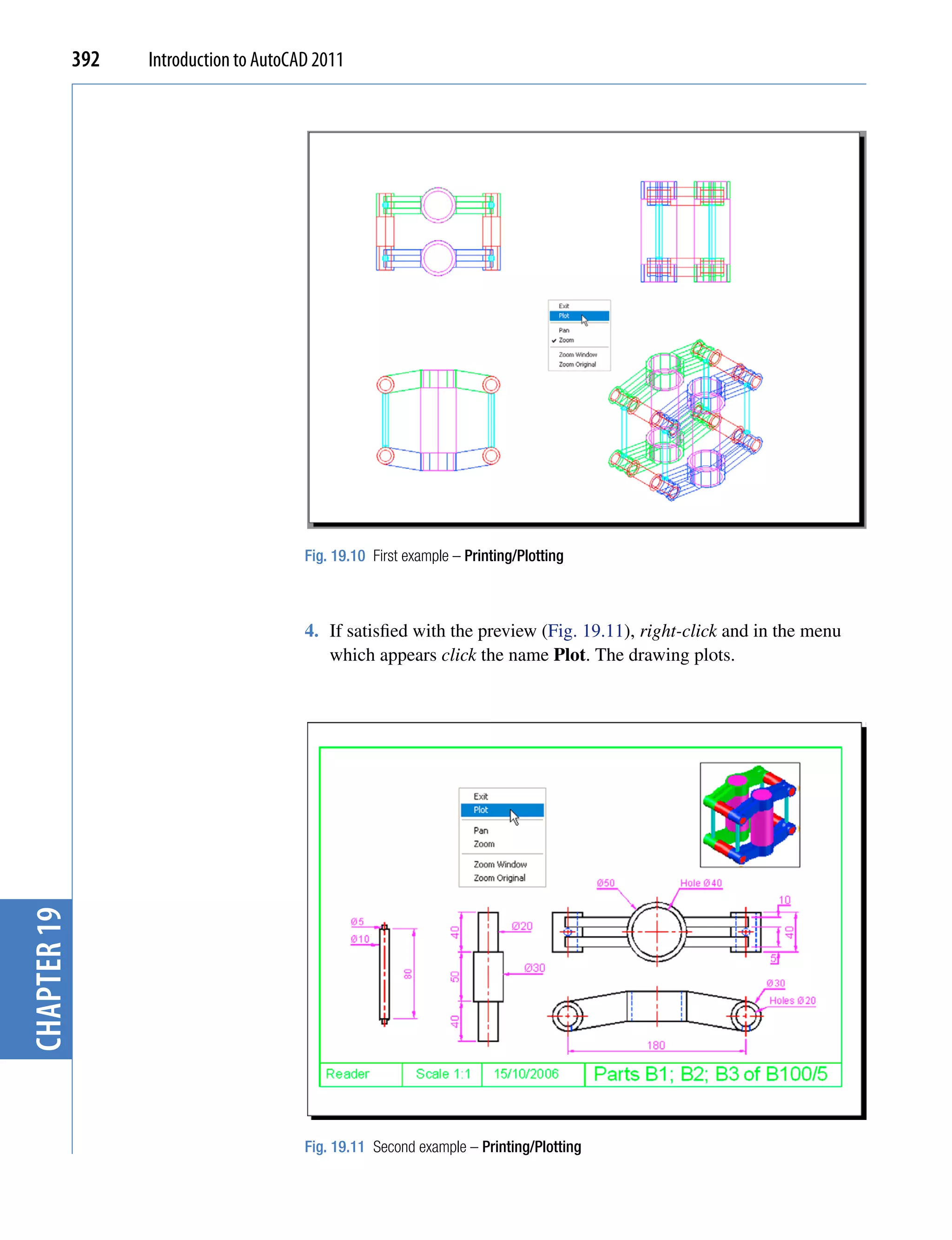
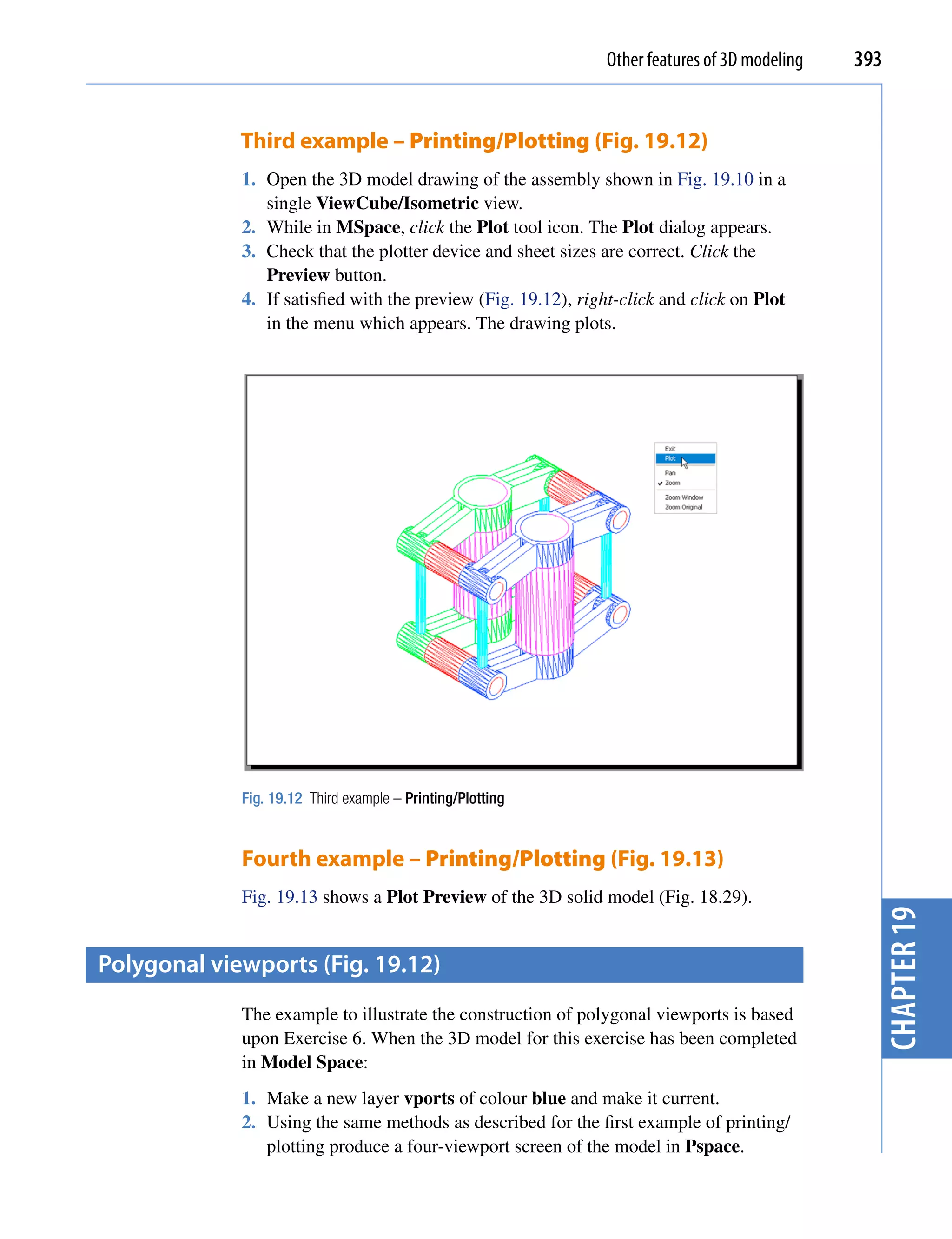
![394 Introduction to AutoCAD 2011
Fig. 19.13 Fourth example – Printing/Plotting
3. Erase the viewport with a click on its bounding line. The outline and its
contents are erased.
4. Click the Model button. With a click in each viewport in turn and
using the ViewCube settings set viewports in Front, Right, Top and
Isometric views, respectively.
5. Zoom each viewport to All.
6. Click the Layout1 button to turn back to PSpace.
7. Enter mv at the command line, which shows:
Command: enter mv right-click
MVIEW
[prompts]: enter p (Polygonal) right-click
Specify start point: In the top right viewport
pick one corner of a square
chapter 19
Specify next point or [Arc/Close/Length/Undo]:
pick next corner for the square
Specify next point or [Arc/Close/Length/Undo]:
pick next corner for the square
Specify next point or [Arc/Close/Length/Undo]:
enter c (Close)right-click
Regenerating model.
Command:
And a square viewport outline appears in the top right viewport within
which is a copy of the model.](https://image.slidesharecdn.com/introductiontoautocad2011-100614022653-phpapp02/75/Introduction-to-AutoCad-2011-384-2048.jpg)
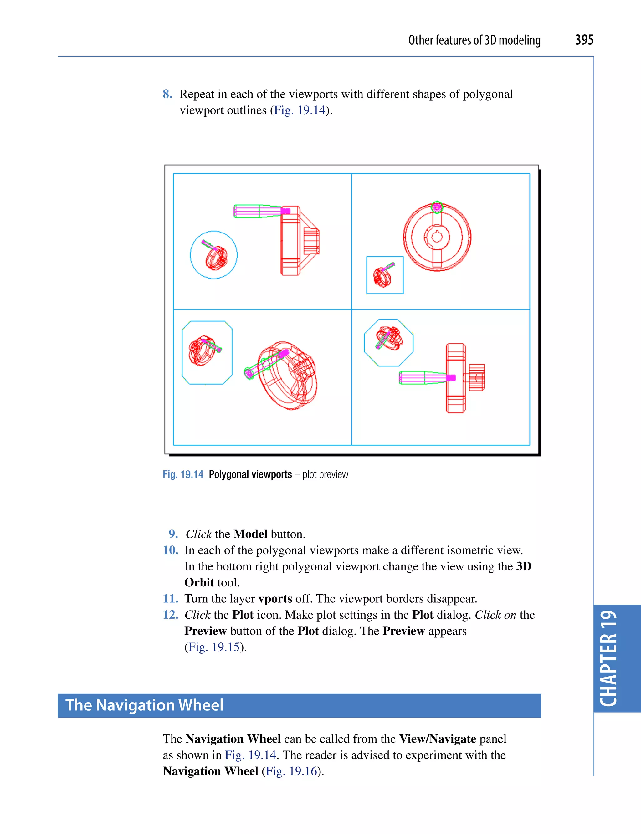
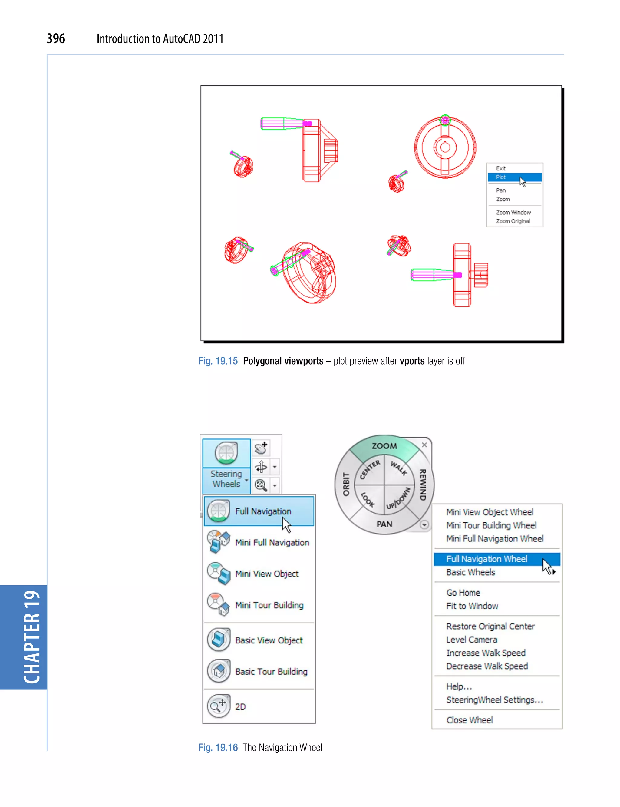
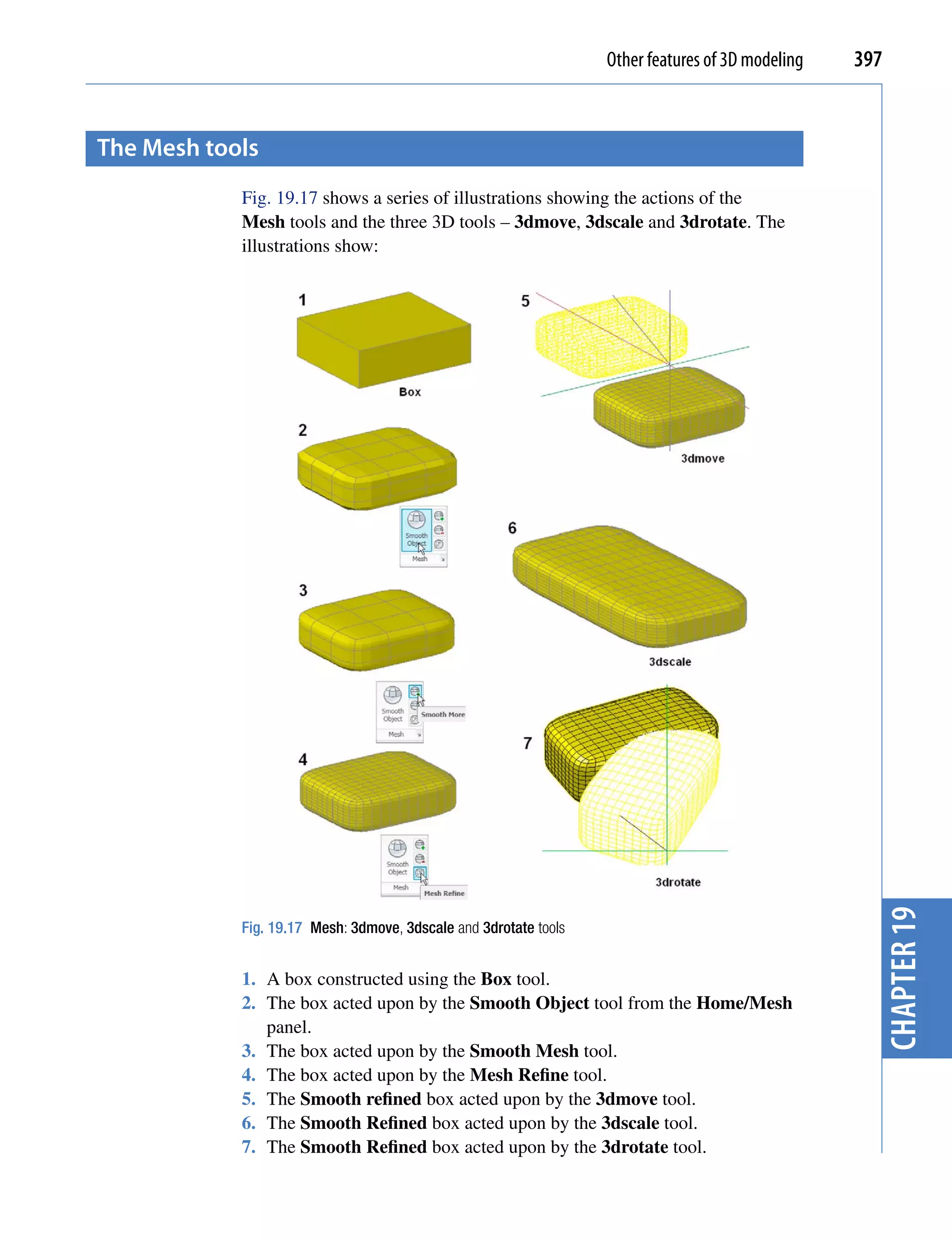
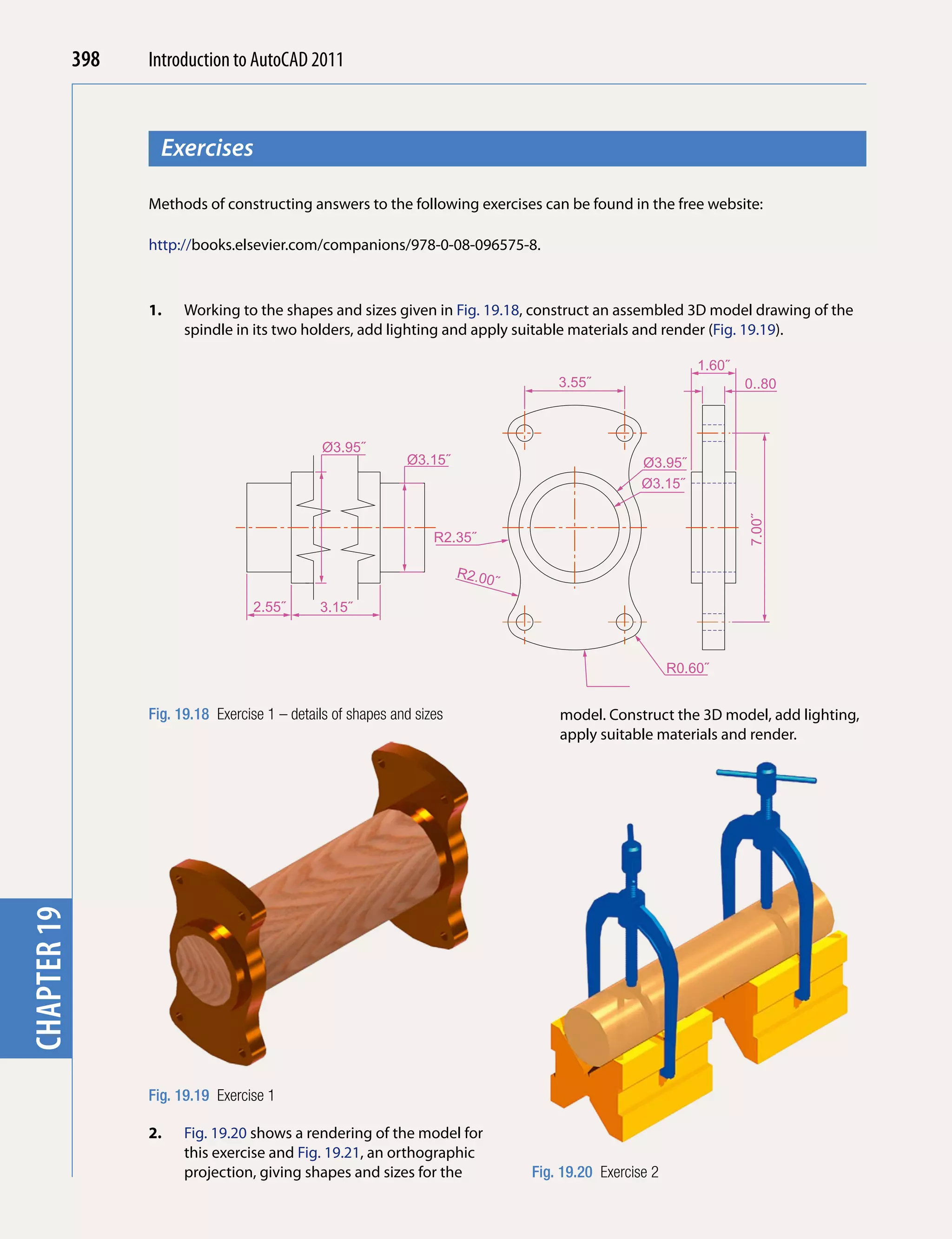
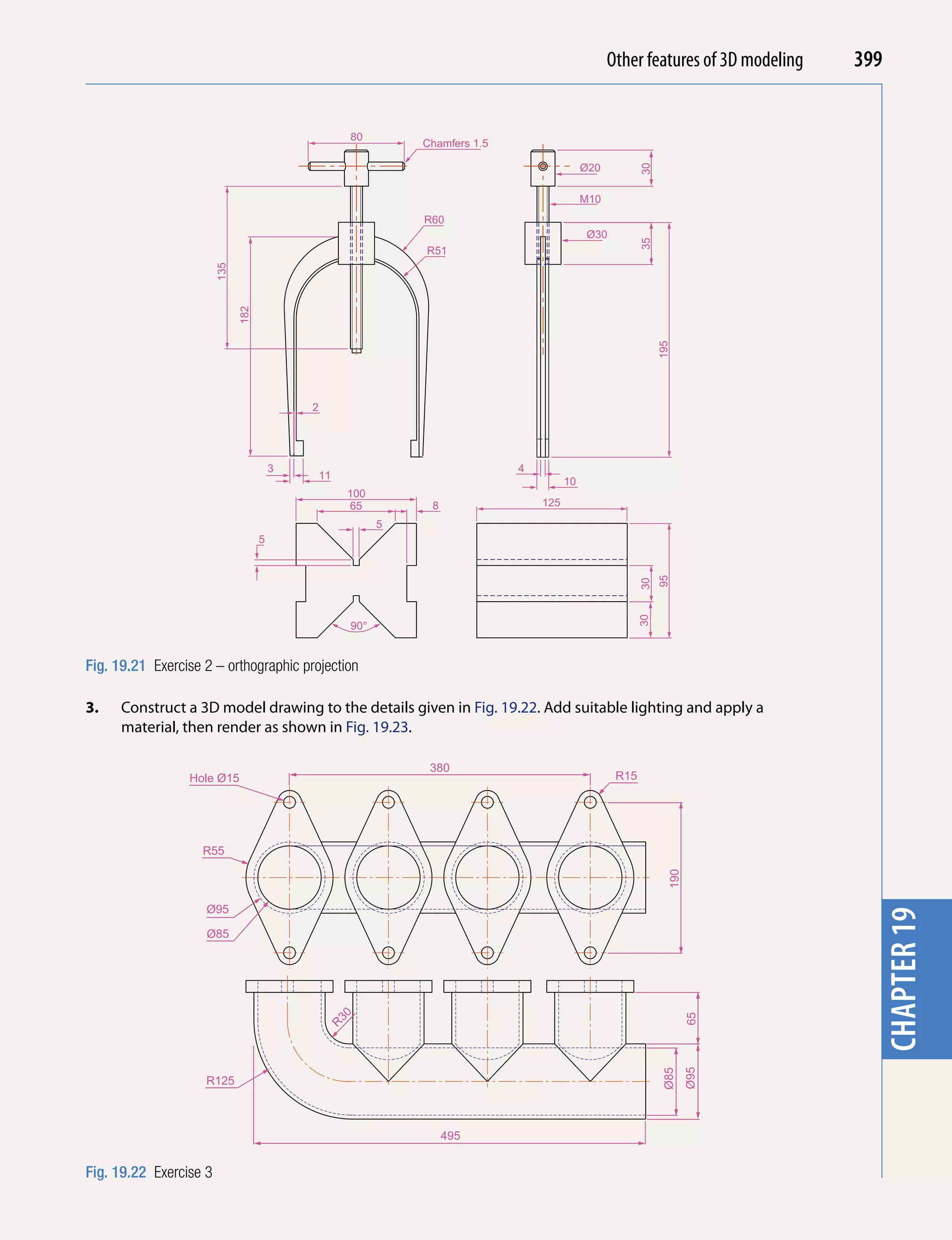
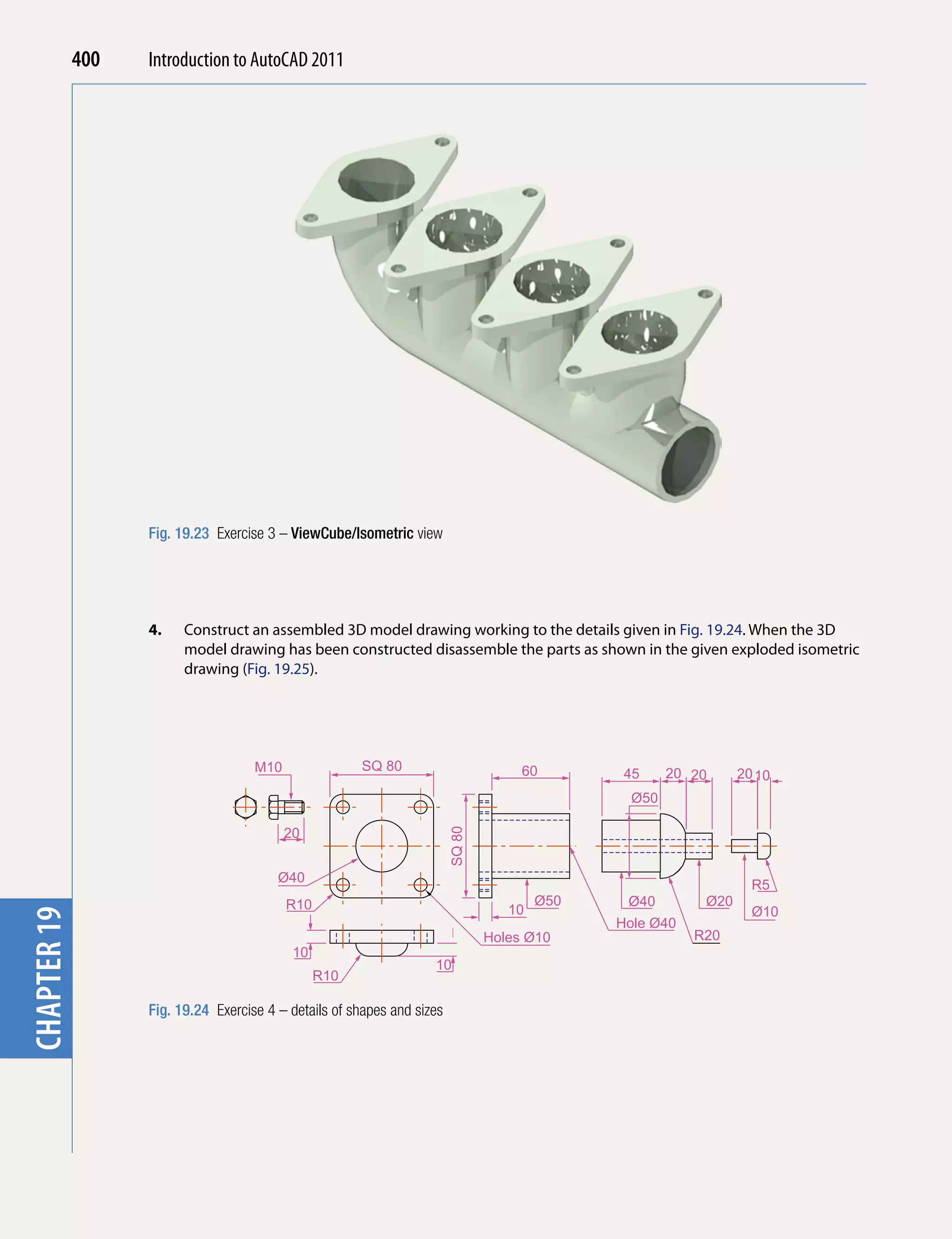
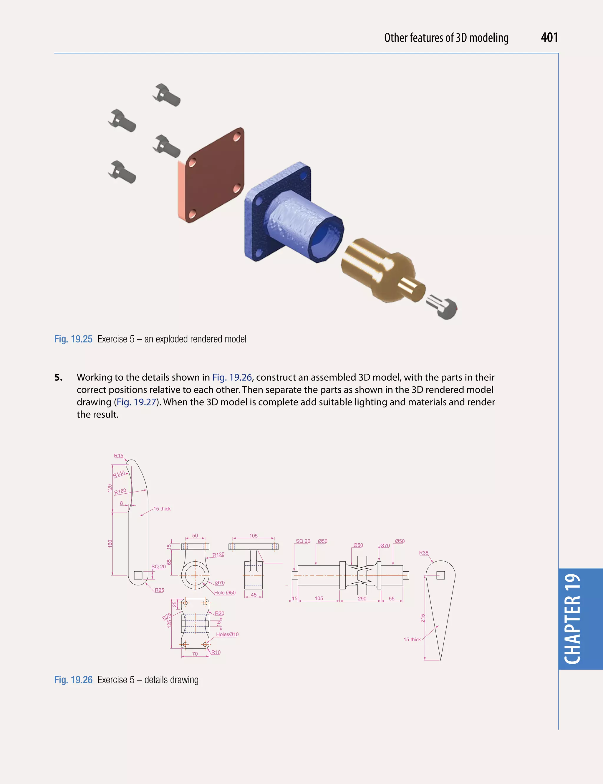
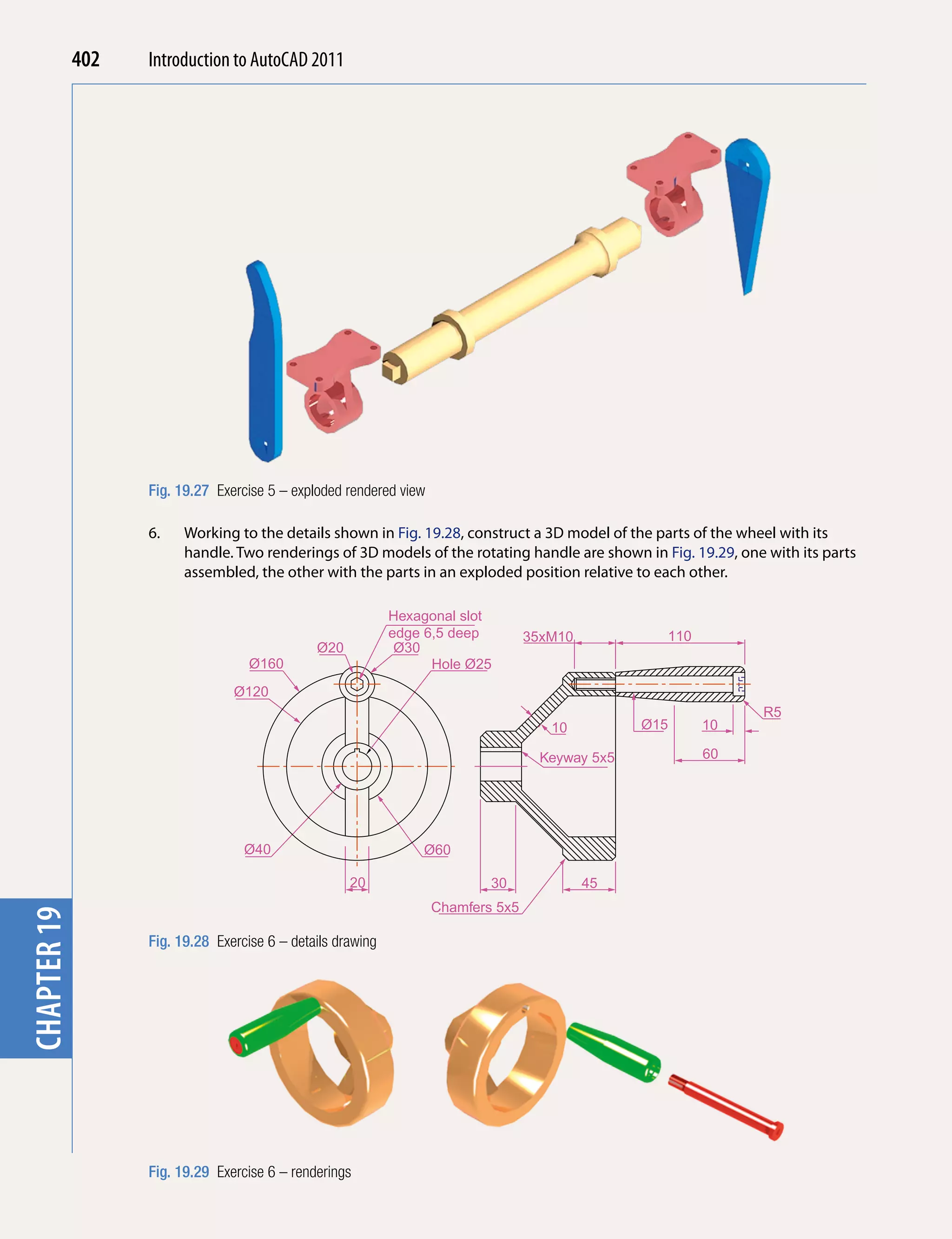

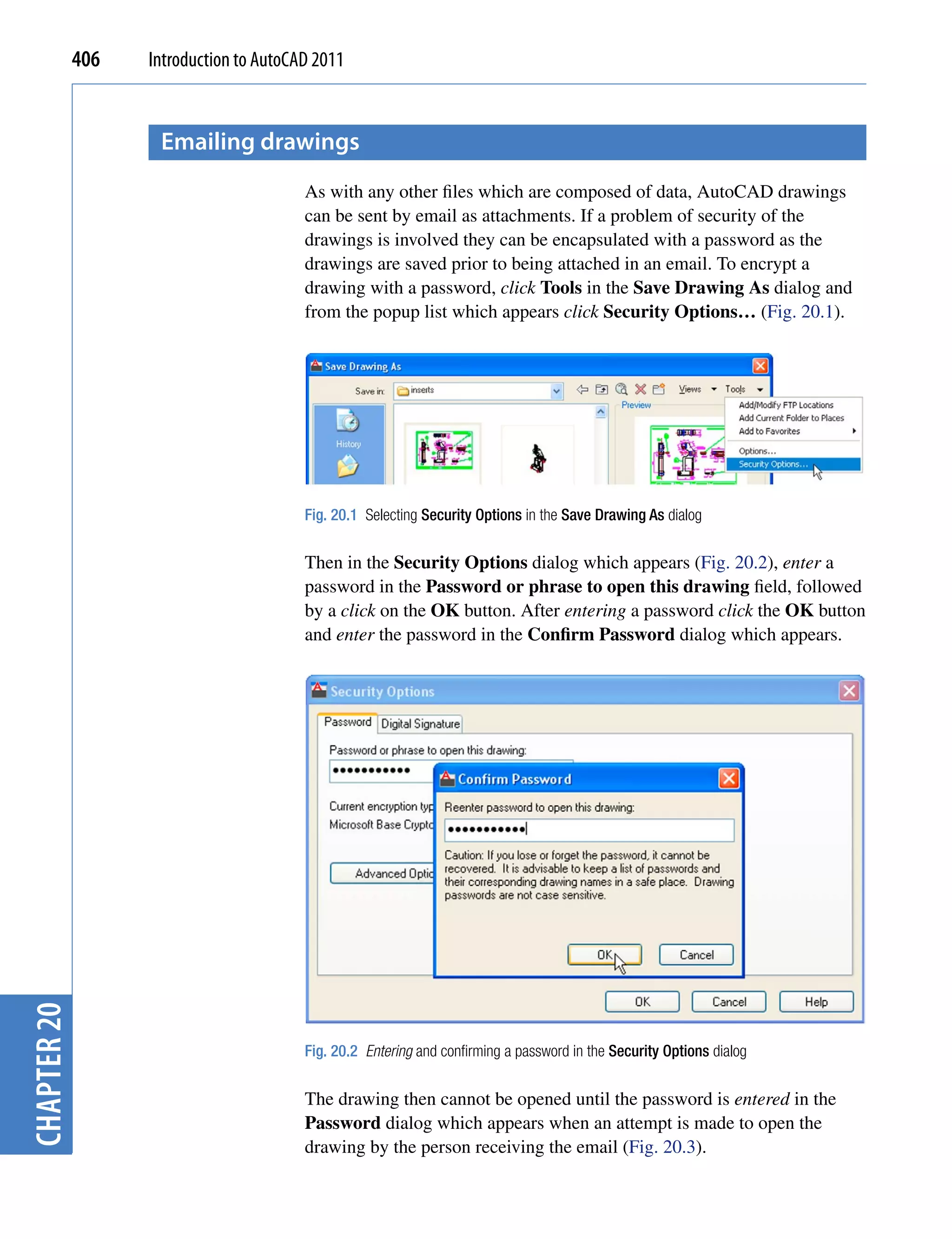
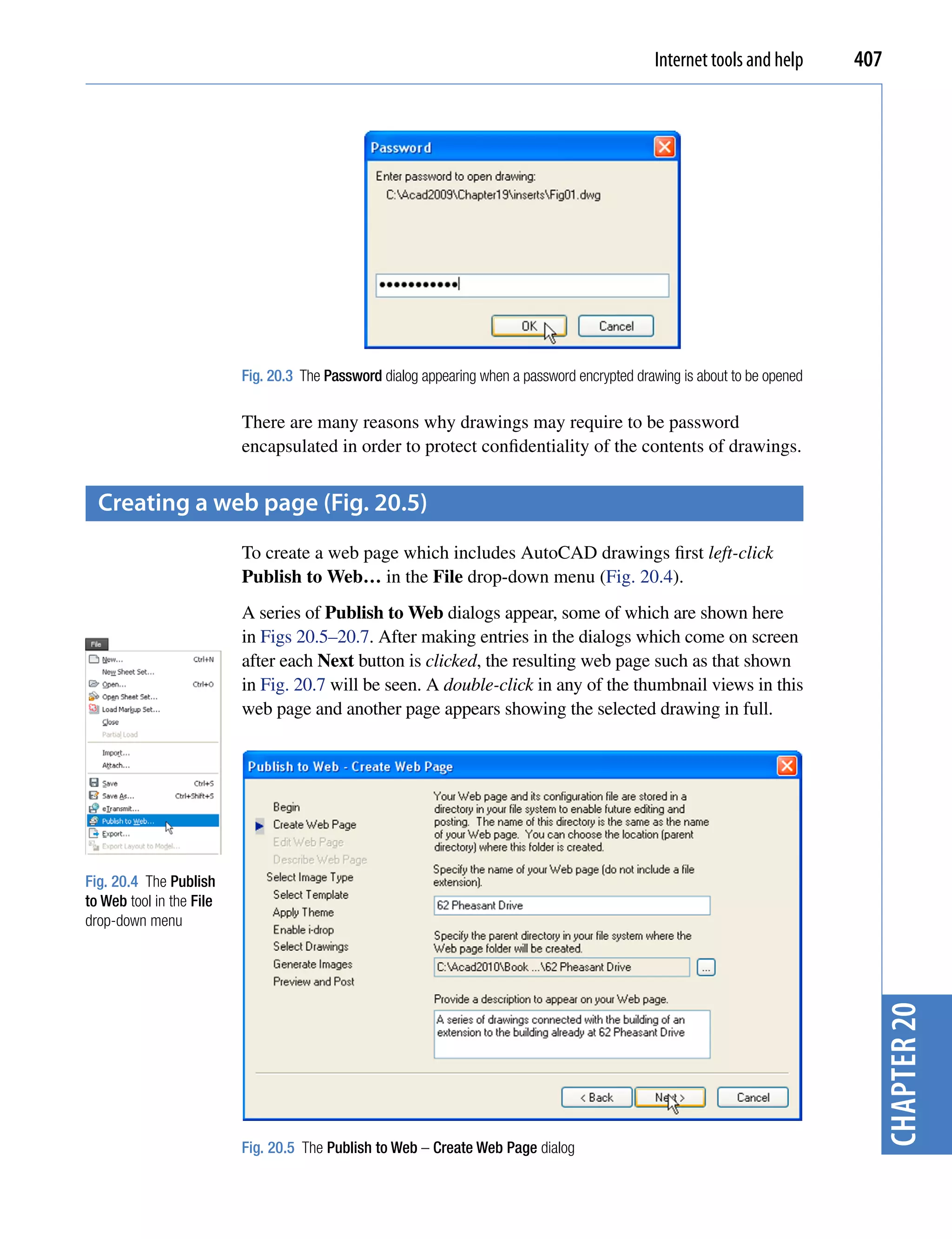
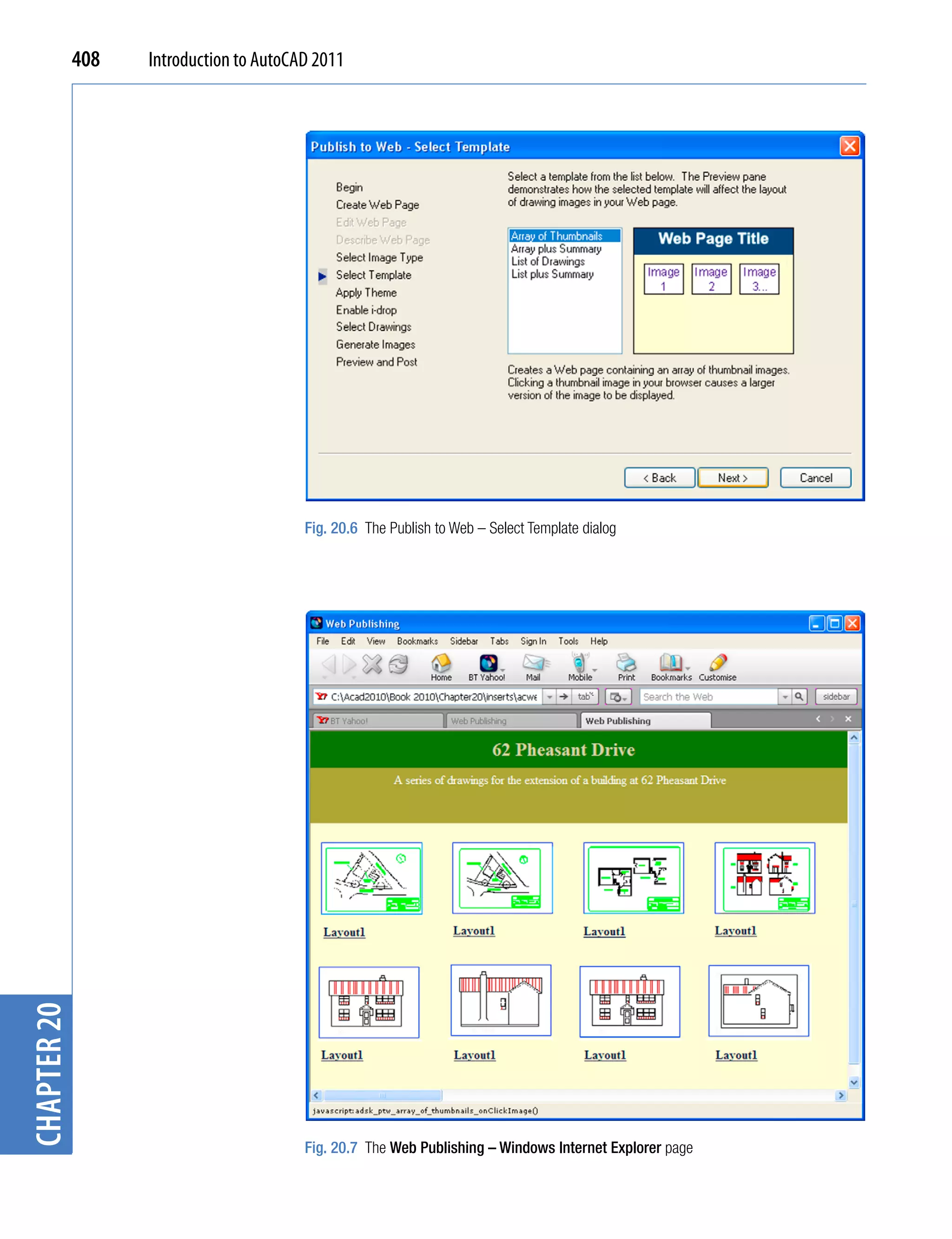
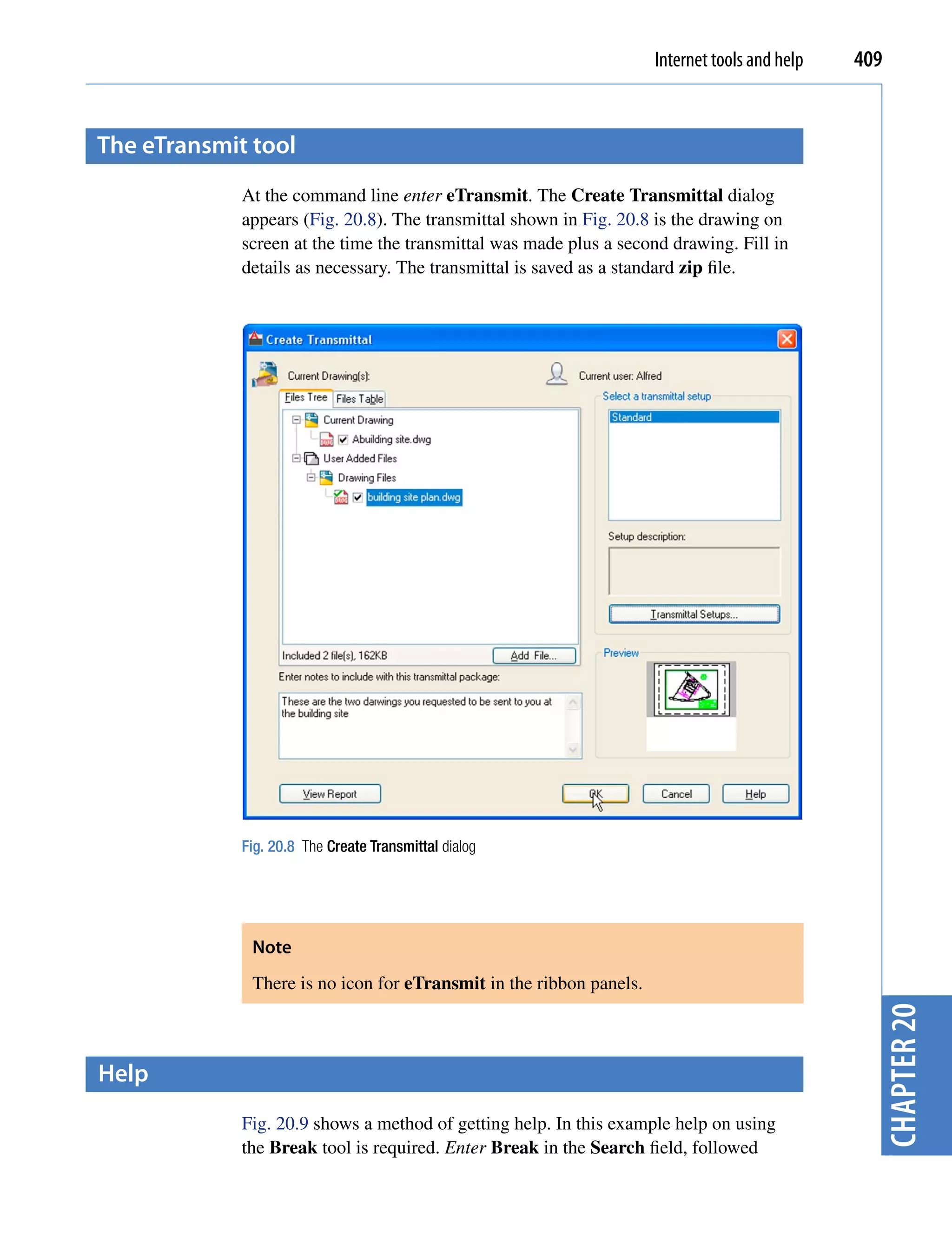
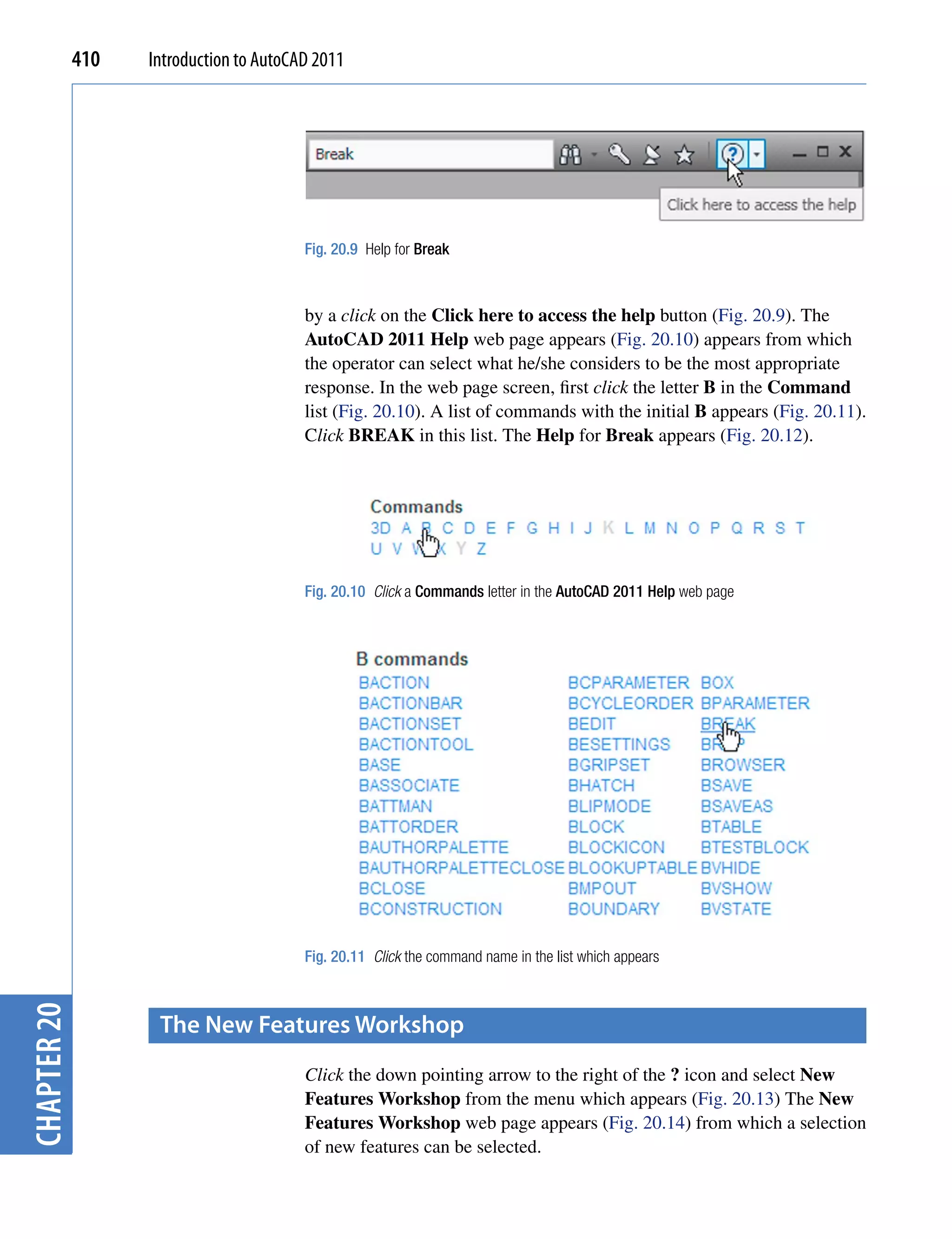
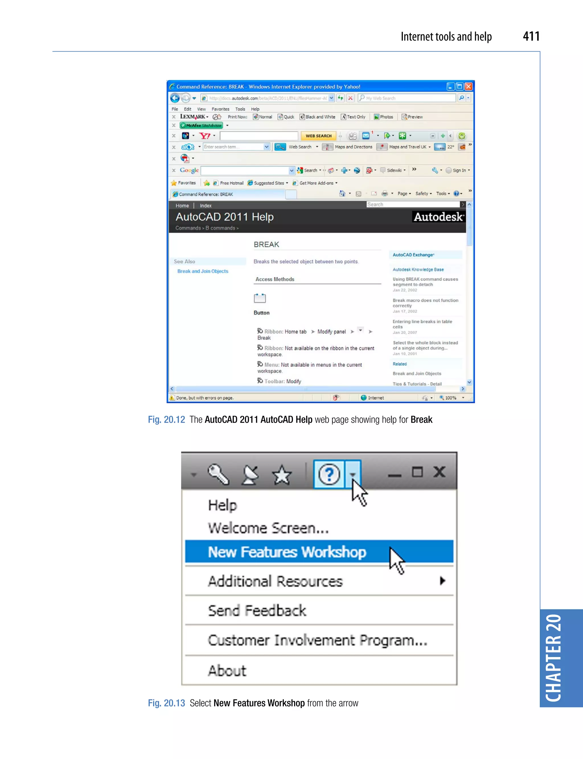
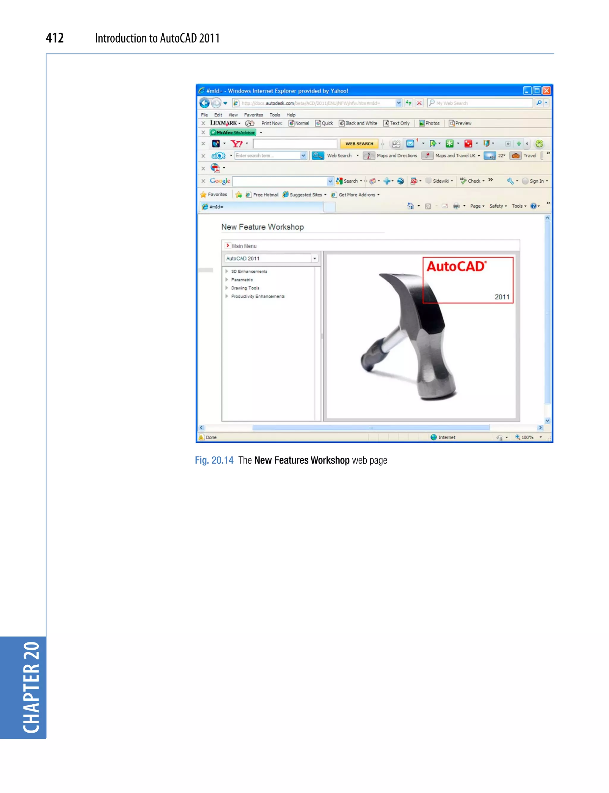
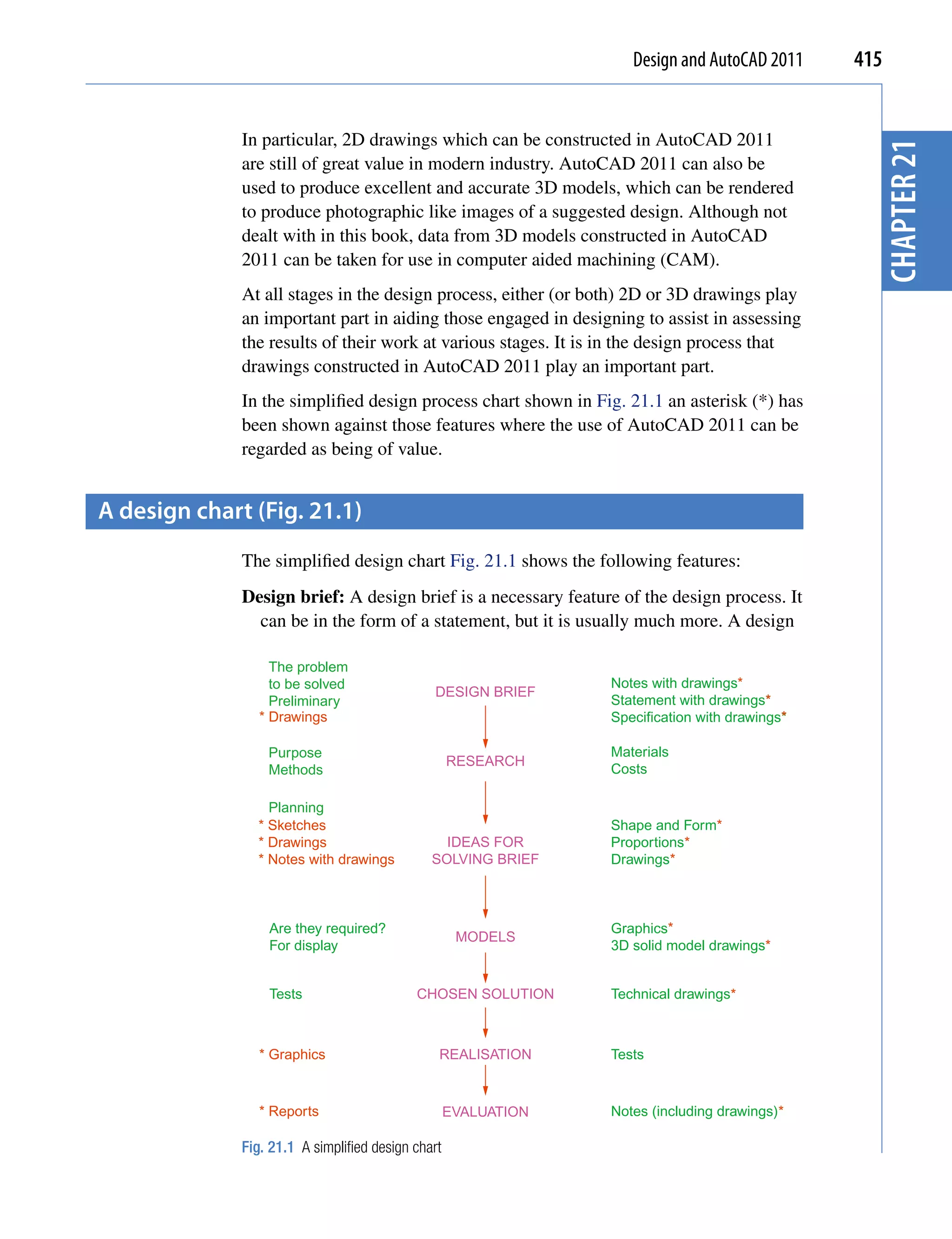


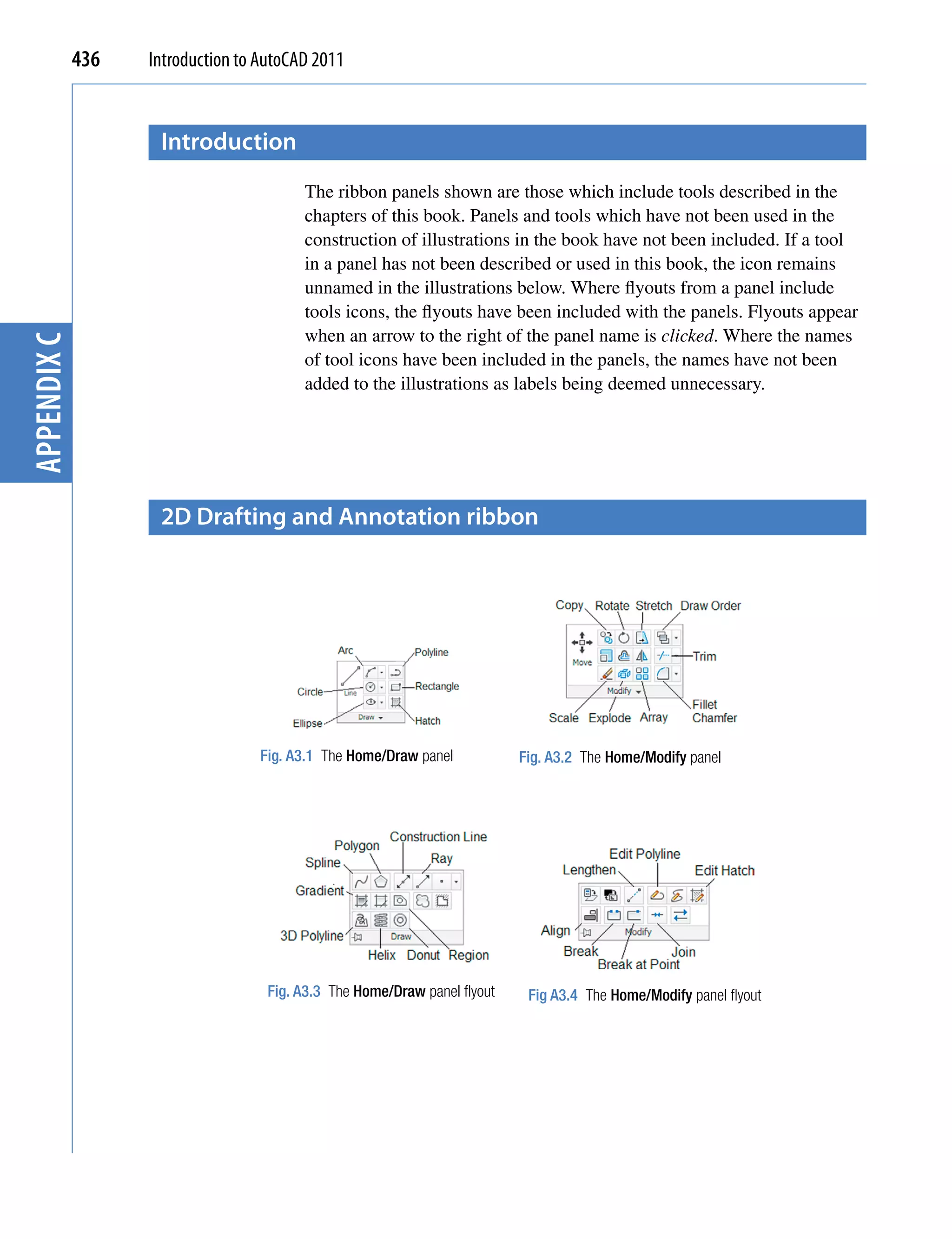
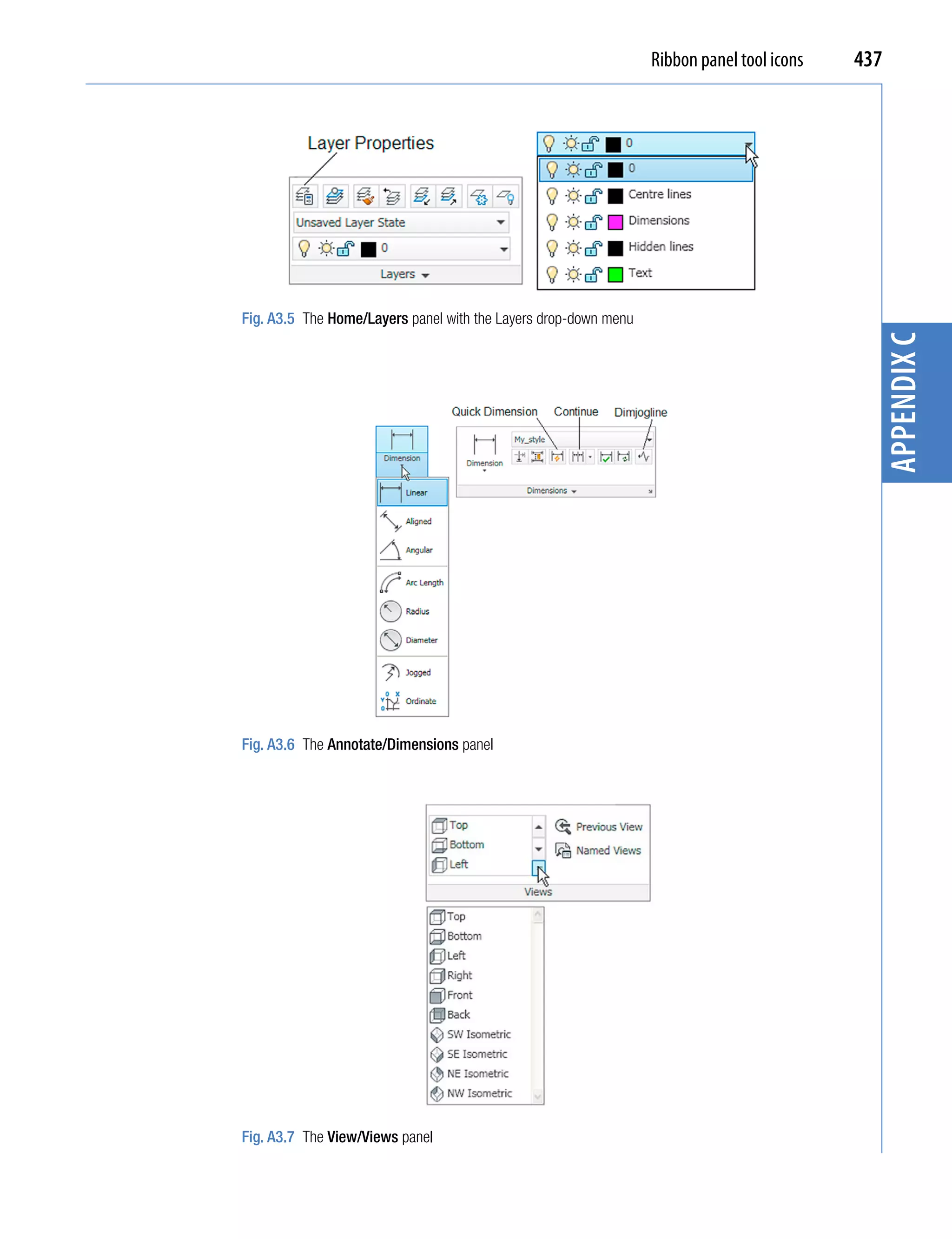
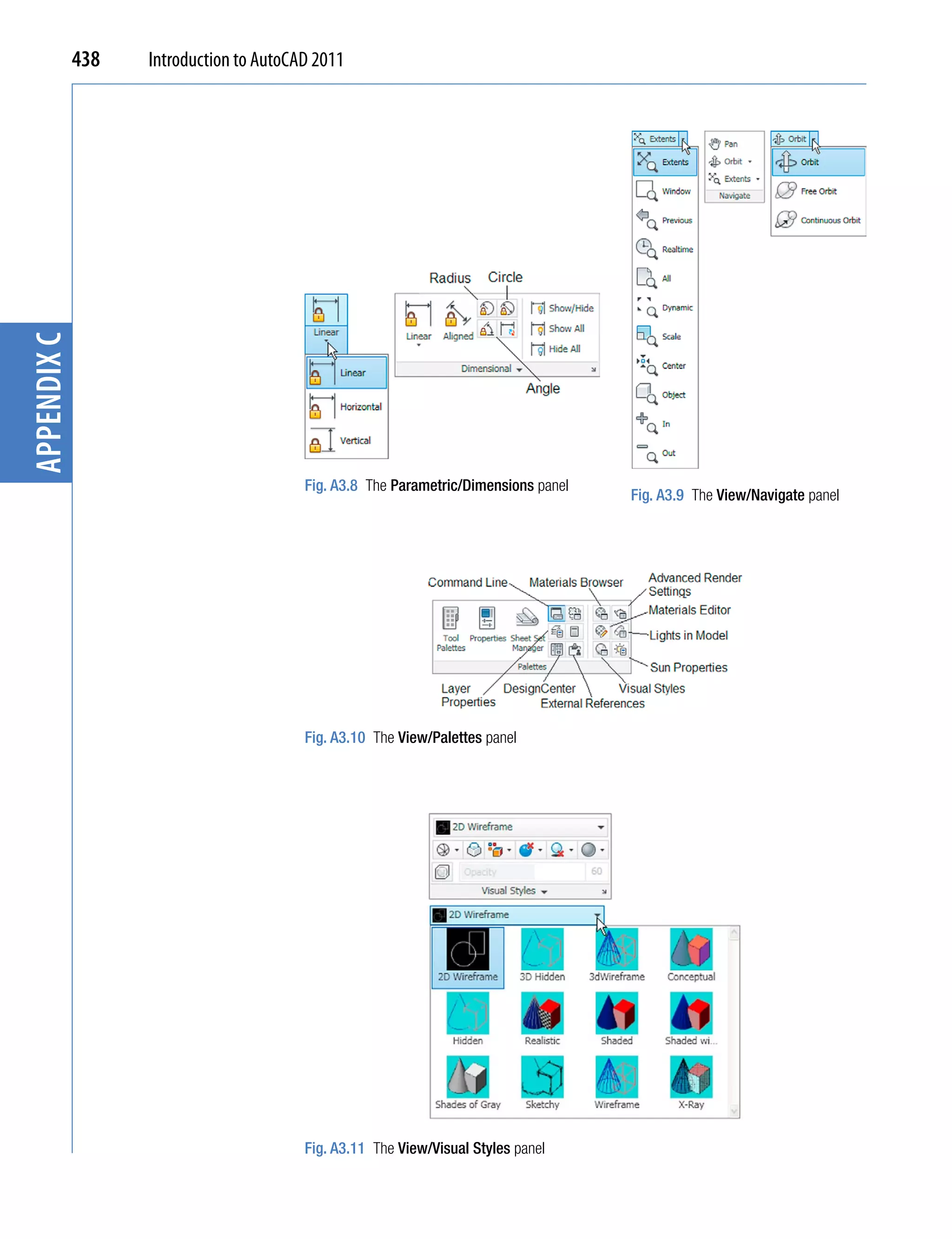
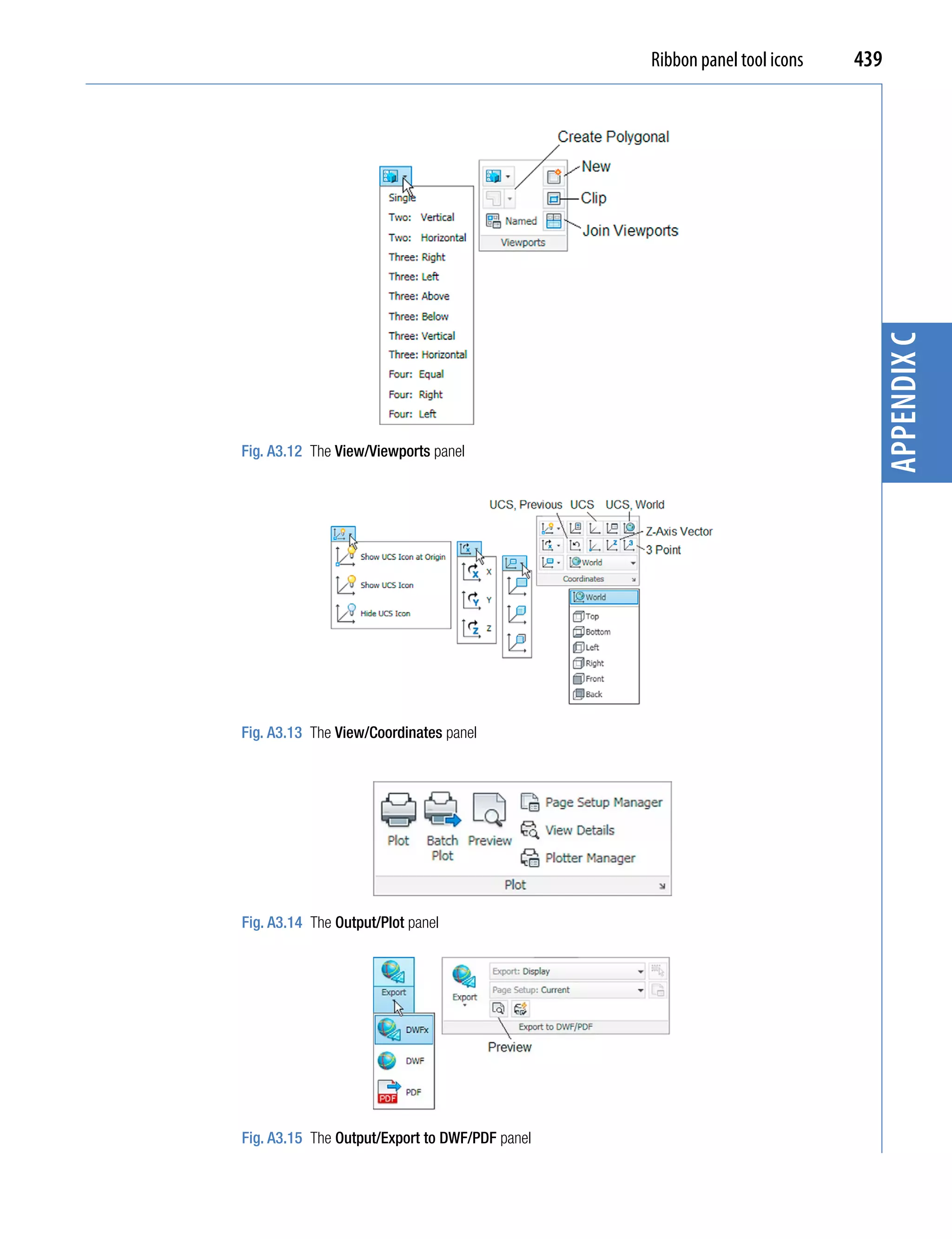
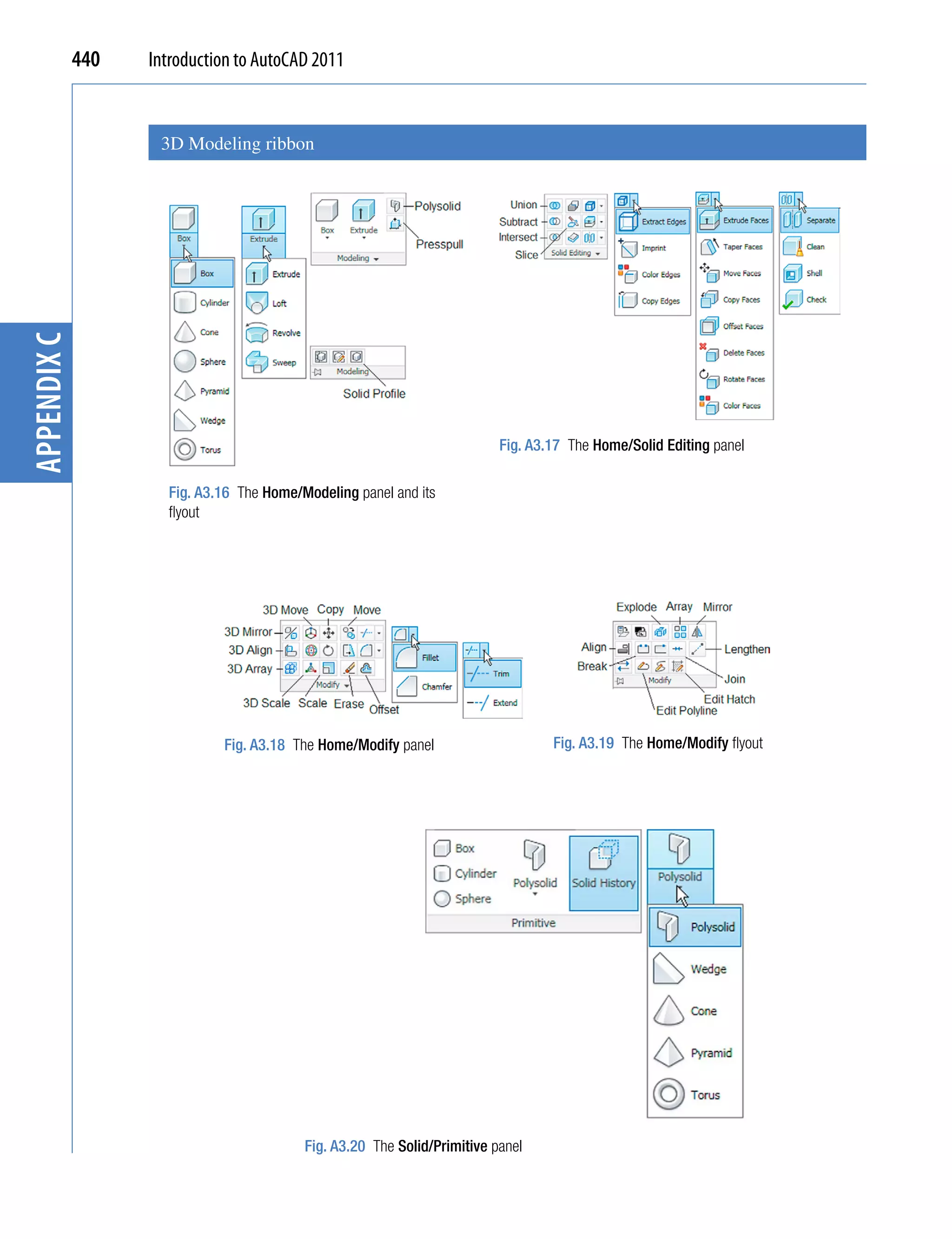
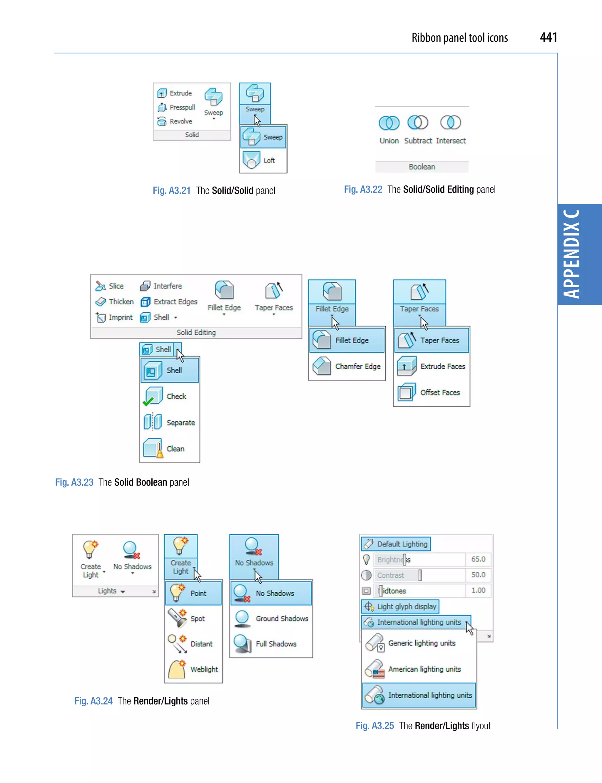
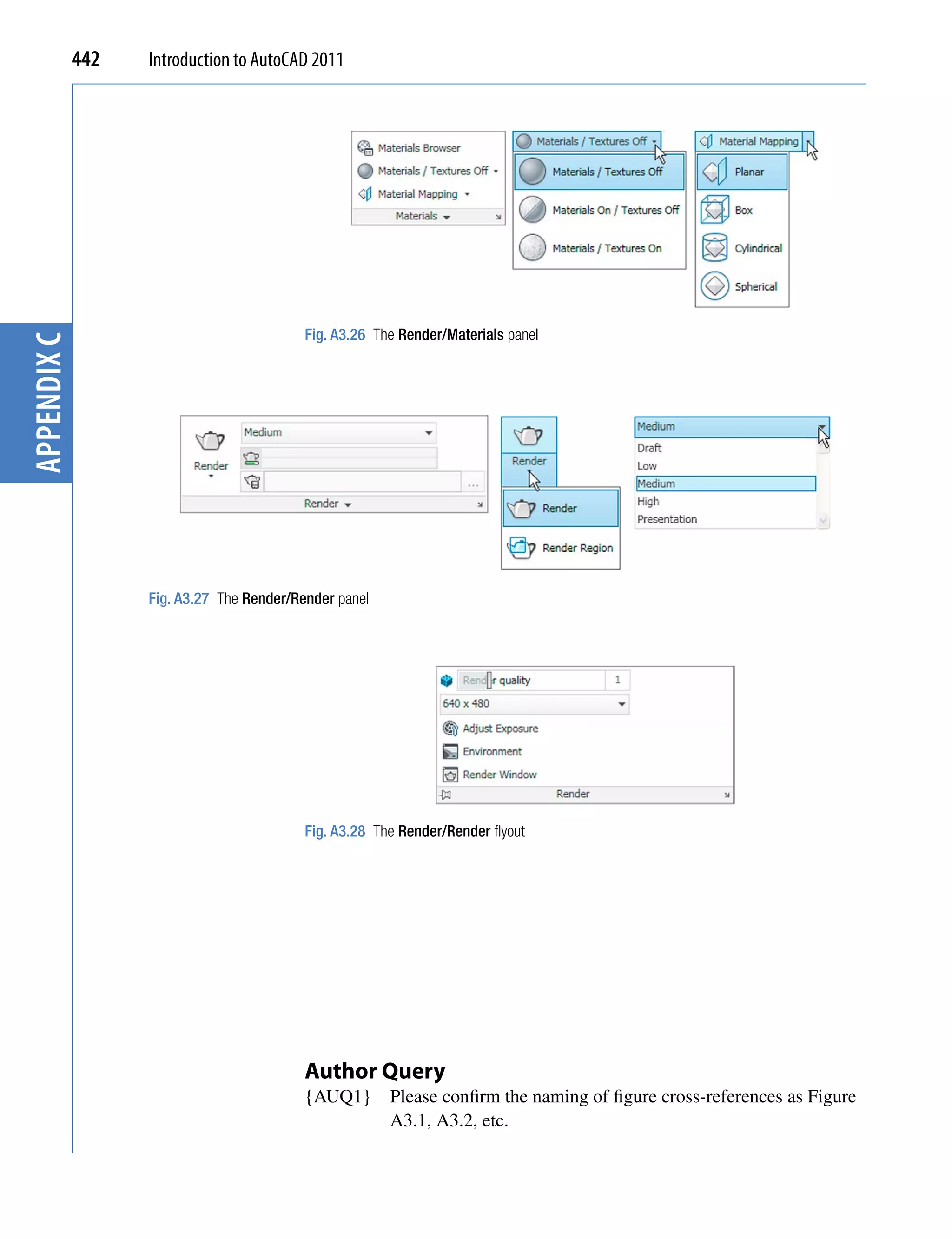

This chapter introduces the features of the AutoCAD 2011 window and methods of operating AutoCAD 2011. It describes opening AutoCAD 2011, the main components of the AutoCAD window including the ribbon, toolbars, menus and panels. It also discusses basic functions like grids, snaps, templates and the coordinate system.