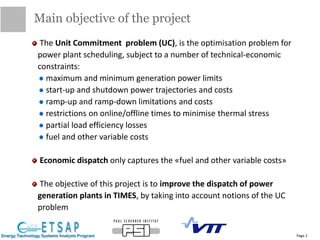
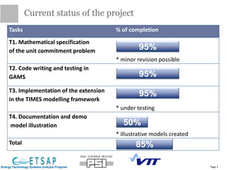
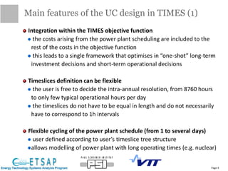
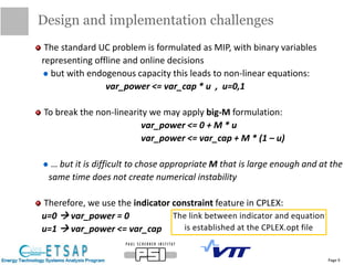
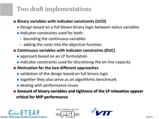
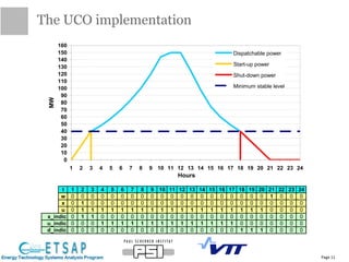
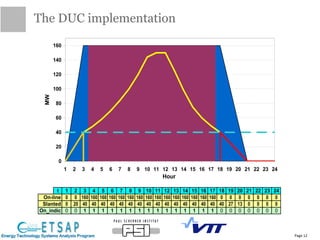
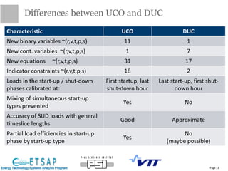
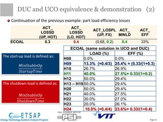
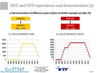
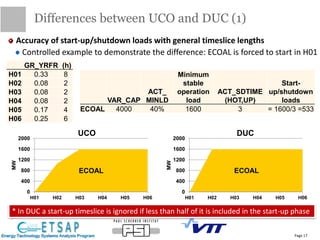
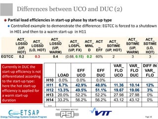
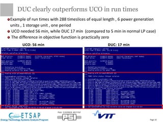
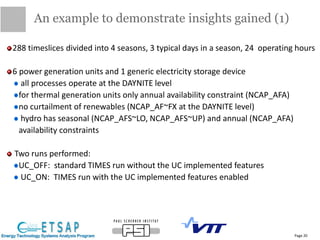
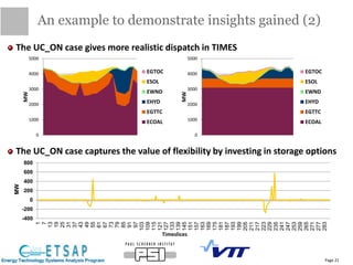
This document provides an update on the status of a project to improve the dispatch modeling of power plants in the TIMES energy systems modeling framework. It describes the implementation of a unit commitment (UC) problem into TIMES, which will allow the model to consider start-up costs and minimum run times of power plants when determining the optimal dispatch schedule. The document outlines the key features and constraints of the UC problem being modeled, provides an overview of the current implementation progress and tasks completed, and describes two different approaches - using binary variables or continuous variables - for formulating the UC problem in TIMES. Examples are also presented to demonstrate the UC modeling capabilities.

1. Dispatching and Unit Commitment
Features in TIMES
69th ETSAP Workshop, UCC, 30-31 May 2016
Update on project´s status
Evangelos Panos, PSI
Antti Lehtilä, VTT

2. The Unit Commitment problem (UC), is the optimisation problem for
power plant scheduling, subject to a number of technical-economic
constraints:
maximum and minimum generation power limits
start-up and shutdown power trajectories and costs
ramp-up and ramp-down limitations and costs
restrictions on online/offline times to minimise thermal stress
partial load efficiency losses
fuel and other variable costs
Economic dispatch only captures the «fuel and other variable costs»
The objective of this project is to improve the dispatch of power
generation plants in TIMES, by taking into account notions of the UC
problem
Main objective of the project
Page 2

3. Current status of the project
Page 3
Tasks % of completion
T1. Mathematical specification
of the unit commitment problem
* minor revision possible
T2. Code writing and testing in
GAMS
T3. Implementation of the extension
in the TIMES modelling framework
* under testing
T4. Documentation and demo
model illustration
* illustrative models created
Total
95%
95%
95%
50%
85%

4. Integration within the TIMES objective function
the costs arising from the power plant scheduling are included to the
rest of the costs in the objective function
this leads to a single framework that optimises in “one-shot” long-term
investment decisions and short-term operational decisions
Timeslices definition can be flexible
the user is free to decide the intra-annual resolution, from 8760 hours
to only few typical operational hours per day
the timeslices do not have to be equal in length and do not necessarily
have to correspond to 1h intervals
Flexible cycling of the power plant schedule (from 1 to several days)
user defined according to user’s timeslice tree structure
allows modelling of power plant with long operating times (e.g. nuclear)
Main features of the UC design in TIMES (1)
Page 4

5. A generation unit does not necessarily correspond to a discrete plant
A unit can change stand-by condition from hot to warm and then to cold
depending on its non-operational time after shutdown
this identifies three different start-up types: hot, warm, cold
Start-up (and synchronisation) phase of a unit:
its duration depends on the chosen start-up type
load is linearly increased up to the minimum stable operation level
start-up costs can occur:
 capacity related  based on the started capacity
 fuel related  due to partial load efficiency losses
Main features of the UC design in TIMES (2)
Page 5

6. Dispatching phase:
load is between the minimum stable operation level and the maximum
available (started) capacity
load changes are subject to ramping limitations
partial load efficiency losses can occur if unit operates below a level
(above which no losses are assumed to occur anymore)
Shutdown (and desynchronisation) phase:
the load is linearly decreased from the minimum stable operation level
 … based on the duration of the phase
Shutdown costs can occur:
 capacity related  based on the started capacity
 fuel related  due to partial load efficiency losses
All UC-related costs are entered into TIMES objective function
Main features of the UC design in TIMES (3)
Page 6

7. Partial load efficiency losses are modelled through a linearly approx. loss in
activity, which is added to increase the fuel consumption:
var_flo * act_eff = var_act + var_actlos
Main features of the UC design in TIMES (4)
Page 7
20%
25%
30%
35%
40%
45%
50%
55%
60%
65%
0% 20% 40% 60% 80% 100%
Efficiency%
Load %
Calculated efficiency % vs load
0.2
2.2
4.2
6.2
8.2
10.2
12.2
14.2
16.2
0% 20% 40% 60% 80% 100%
AdditionalActivity
Load %
Calculated loss in activity vs load
1) At the start-up load the activity loss is calibrated to the start-up efficiency
2) Then the activity loss decreases linearly to the losses at the minimum stable operation level
3) The loss at the minimum stable operation level equals to var_act
4) Then the activity loss is linearly decreased to 0

8. New TIMES user-defined parameters
Page 8
Parameter Explanation Unit
G_CYCLE (tslv) Number of cycles in an average year
(ANNUAL=1, WEEKLY=365/7, DAYNITE=365)
Number of cycles in each
timeslice level
ACT_MINLD (r,v,p) Minimum stable operation level % of online capacity
ACT_UPS (r,v,p,bd) Ramp up (bd=UP) and ramp down (bd=LO)
rates
% of online capacity
ACT_MAXNON (r,v,p,upt) Maximum non-operational time before
start-up type (upt=HOT, WARM, COLD)
Hours when DAYNITE
Days when WEEKLY
ACT_SDTIME (r,v,p,upt,bd) Duration of start-up and shut-down phases Hours
ACT_CSTRAMP (r,v,p,bd,cur) Ramp up (bd=UP) and ramp down (bd=LO)
costs
Cost per unit of power
output
ACT_CSTSD
(r,v,p,upt,bd,cur)
Start up (bd=UP) costs per start-up type upt
and shut down (bd=LO) costs
Cost per unit of started-up
capacity
ACT_LOSPL (r,v,p,bd) Partial load efficiency loss at the dispatching
phase
% of increase in specific
fuel consumption
ACT_LOSSD (r,v,p,upt,bd) Partial load efficiency loss at the start-
up/shut-down phases
% of increase in specific
fuel consumption

9. The standard UC problem is formulated as MIP, with binary variables
representing offline and online decisions
but with endogenous capacity this leads to non-linear equations:
var_power <= var_cap * u , u=0,1
To break the non-linearity we may apply big-M formulation:
var_power <= 0 + M * u
var_power <= var_cap + M * (1 – u)
… but it is difficult to chose appropriate M that is large enough and at the
same time does not create numerical instability
Therefore, we use the indicator constraint feature in CPLEX:
u=0  var_power = 0
u=1  var_power <= var_cap
Design and implementation challenges
Page 9
The link between indicator and equation
is established at the CPLEX.opt file

10. Binary variables with indicator constraints (UCO)
Design based on a full-blown binary logic between status variables
Indicator constraints used for both:
 bounding the continuous variables
 adding the costs into the objective function
Continuous variables with indicator constraints (DUC)
approach based on an LP formulation
indicator constraints used for discretising the on-line capacity
Motivation for the two different approaches
validation of the design based on full binary logic
together they also serve as an algorithmic benchmark
dealing with performance issues
Amount of binary variables and tightness of the LP relaxation appear
critical for MIP performance
Two draft implementations
Page 10

11. The UCO implementation
Page 11
0
10
20
30
40
50
60
70
80
90
100
110
120
130
140
150
160
1 2 3 4 5 6 7 8 9 10 11 12 13 14 15 16 17 18 19 20 21 22 23 24
Hours
MW Dispatchable power
Start-up power
Shut-down power
Minimum stable level
t 1 2 3 4 5 6 7 8 9 10 11 12 13 14 15 16 17 18 19 20 21 22 23 24
w 0 0 0 0 0 0 0 0 0 0 0 0 0 0 0 0 0 0 0 0 1 0 0 0
x 0 1 0 0 0 0 0 0 0 0 0 0 0 0 0 0 0 0 0 0 0 0 0 0
u 0 1 1 1 1 1 1 1 1 1 1 1 1 1 1 1 1 1 1 1 0 0 0 0
x_indic 0 1 1 0 0 0 0 0 0 0 0 0 0 0 0 0 0 0 0 0 0 0 0 0
u_indic 0 0 0 1 1 1 1 1 1 1 1 1 1 1 1 1 1 0 0 0 0 0 0 0
d_indic 0 0 0 0 0 0 0 0 0 0 0 0 0 0 0 0 0 1 1 1 0 0 0 0

12. The DUC implementation
Page 12
0
20
40
60
80
100
120
140
160
1 2 3 4 5 6 7 8 9 10 11 12 13 14 15 16 17 18 19 20 21 22 23 24
Hour
MW
t 1 2 3 4 5 6 7 8 9 10 11 12 13 14 15 16 17 18 19 20 21 22 23 24
On-line 0 0 160 160 160 160 160 160 160 160 160 160 160 160 160 160 160 0 0 0 0 0 0 0
Slanted 0 20 40 40 40 40 40 40 40 40 40 40 40 40 40 40 40 40 27 13 0 0 0 0
On_indic 0 0 1 1 1 1 1 1 1 1 1 1 1 1 1 1 1 0 0 0 0 0 0 0

13. Characteristic UCO DUC
New binary variables ~(r,v,t,p,s) 11 1
New cont. variables ~(r,v,t,p,s) 1 7
New equations ~(r,v,t,p,s) 31 17
Indicator constraints ~(r,v,t,p,s) 18 2
Loads in the start-up / shut-down
phases calibrated at:
First startup, last
shut-down hour
Last start-up, first shut-
down hour
Mixing of simultaneous start-up
types prevented
Yes No
Accuracy of SUD loads with general
timeslice lengths
Good Approximate
Partial load efficiencies in start-up
phase by start-up type
Yes
No
(maybe possible)
Differences between UCO and DUC
Page 13

14. 0
400
800
1200
1600
2000
2400
H01
H02
H03
H04
H05
H06
H07
H08
H09
H10
H11
H12
H13
H14
H15
H16
H17
H18
H19
H20
H21
H22
H23
H24
MW
DUC (VAR_OBJ=18987987)
ECOAL
To demonstrate the features in TIMES a controlled example is presented
In this example the ECOAL unit is forced to shutdown in H01 and start-up in H09
DUC and UCO equivalence & demonstration (1)
Page 14
NCAP_
PASTI
ACT_
MNLD
Minimum stable
operation load
ACT_
UPS
ACT_SDTIME
(UP, HOT)
ACT_SDTIME
(LO, HOT)
ECOAL 4000 40% 1600 10% 3 4
0
400
800
1200
1600
2000
2400
H01
H02
H03
H04
H05
H06
H07
H08
H09
H10
H11
H12
H13
H14
H15
H16
H17
H18
H19
H20
H21
H22
H23
H24
MW
UCO (VAR_OBJ=18987974)
Note: in the graphs the other units have been ommitted
ECOAL

15. Continuation of the previous example: part load efficiency losses
DUC and UCO equivalence & demonstration (2)
Page 15
ACT_
LOSSD
(UP, HOT)
ACT_
LOSSD
(LO, HOT)
ACT_LOSPL
(UP, FX)
ACT_
MINLD
ACT_
EFF
ECOAL 0.3 0.4 (0.68, 0.2) 0.4 33%
The start-up load is defined as:
𝑀𝑖𝑛𝑆𝑡𝑎𝑏𝑙𝑒𝑂𝑝
𝑆𝑡𝑎𝑟𝑡𝑢𝑝𝑇𝑖𝑚𝑒
The shutdown load is defined as:
𝑀𝑖𝑛𝑆𝑡𝑎𝑏𝑙𝑒𝑂𝑝
𝑆ℎ𝑢𝑡𝑑𝑜𝑤𝑛𝑇𝑖𝑚𝑒
ECOAL (same solution in UCO and DUC)
LOAD (%) EFF (%)
H08 0.0% 0.0%
H09 13.3% (=0.4/3) 25.4% = (0.33/(1+0.3)
H10 26.7% 26.9%
H11 40.0% 27.5%= 0.33/(1+0.2)
H12 50.0% 29.4%
H13 – H19 50.0% 29.4%
H20 50.0% 29.4%
H21 40.0% 27.5%
H22 30.0% 27.0%
H23 20.0% 26.1%
H24 10.0% (=0.4/4) 23.6%= 0.33/(1+0.4)

16. Demonstration of different cycles (refers to ECOAL example of slide 14)
DUC and UCO equivalence and demonstration (3)
Page 16
ANNUAL
DAYNITE
H01…H24
G_CYCLE(‘DAYNITE’)=365
ANNUAL
DAYNITE
H01…H48
G_CYCLE(‘DAYNITE’)=365/2
0
500
1000
1500
2000
2500
H01
H03
H05
H07
H09
H11
H13
H15
H17
H19
H21
H23
0
500
1000
1500
2000
2500
3000
3500
4000
H01
H05
H09
H13
H17
H21
H25
H29
H33
H37
H41
H45

17. ECOAL
0
400
800
1200
1600
2000
H01 H02 H03 H04 H05 H06
MW
UCO
ECOAL
0
400
800
1200
1600
2000
H01 H02 H03 H04 H05 H06
MW
DUC
Accuracy of start-up/shutdown loads with general timeslice lengths
Controlled example to demonstrate the difference: ECOAL is forced to start in H01
Differences between UCO and DUC (1)
Page 17
GR_YRFR (h)
H01 0.33 8
H02 0.08 2
H03 0.08 2
H04 0.08 2
H05 0.17 4
H06 0.25 6
VAR_CAP
ACT_
MINLD
Minimum
stable
operation
load
ACT_SDTIME
(HOT,UP)
Start-
up/shutdown
loads
ECOAL 4000 40% 1600 3 = 1600/3 =533
* In DUC a start-up timeslice is ignored if less than half of it is included in the start-up phase

18. Differences between UCO and DUC (2)
Page 18
Partial load efficiencies in start-up phase by start-up type
Controlled example to demonstrate the difference: EGTCC is forced to a shutdown
in H01 and then to a warm start-up in H11
ACT_
LOSSD
(UP,
HOT)
ACT_
LOSSD
(LO, HOT)
ACT_
LOSSD
(UP,
WARM)
ACT_
LOSPL
(UP, FX)
ACT_
MINL
D
ACT
_
EFF
ACT_
SDTIME
(UP, HOT)
ACT_
SDTIME
(UP,
WARM)
ACT_
SDTIME
(LO,
HOT)
EGTCC 0.2 0.3 0.4 (0.68, 0.15) 0.2 60% 2 3 3
LOAD
EFF
UCO
EFF
DUC
VAR_
FLO
UCO
VAR_
FLO
DUC
DIFF IN
VAR_
FLO
H10 0.0% 0.0% 0.0%
H11 6.7% 42.9% 48.0% 11.36 10.14 12%
H12 13.3% 49.5% 51.1% 19.67 19.06 3%
H13 20.0% 52.2% 52.2% 27.98 27.98 0%
H14 33.2% 56.2% 56.2% 43.12 43.12 0%
…
Currently in DUC the
start-up efficiency is not
differentiated according
to the start-up type:
here the hot start-up
efficiency is applied for
a warm start-up
duration

19. Example of run times with 288 timeslices of equal length , 6 power generation
units , 1 storage unit , one period
UCO needed 56 min, while DUC 17 min (compared to 5 min in normal LP case)
The difference in objective function is practically zero
DUC clearly outperforms UCO in run times
Page 19
DUC: 17 minUCO: 56 min

20. 288 timeslices divided into 4 seasons, 3 typical days in a season, 24 operating hours
6 power generation units and 1 generic electricity storage device
all processes operate at the DAYNITE level
for thermal generation units only annual availability constraint (NCAP_AFA)
no curtailment of renewables (NCAP_AF~FX at the DAYNITE level)
hydro has seasonal (NCAP_AFS~LO, NCAP_AFS~UP) and annual (NCAP_AFA)
availability constraints
Two runs performed:
UC_OFF: standard TIMES run without the UC implemented features
UC_ON: TIMES run with the UC implemented features enabled
An example to demonstrate insights gained (1)
Page 20

21. An example to demonstrate insights gained (2)
Page 21
The UC_ON case gives more realistic dispatch in TIMES
The UC_ON case captures the value of flexibility by investing in storage options
0
1000
2000
3000
4000
5000
MW
EGTOC
ESOL
EWND
EHYD
EGTTC
ECOAL
0
1000
2000
3000
4000
5000
MW
EGTOC
ESOL
EWND
EHYD
EGTTC
ECOAL
-400
-200
0
200
400
600
800
1
7
13
19
25
31
37
43
49
55
61
67
73
79
85
91
97
103
109
115
121
127
133
139
145
151
157
163
169
175
181
187
193
199
205
211
217
223
229
235
241
247
253
259
265
271
277
283
MW
Timeslices

22. The UC features make TIMES a unique tool that combines long-term and short-
term decisions in a single and consistent framework
The UCO and DUC implementations can have their own merits, but DUC seems
to be more appropriate for TIMES models
key factors influencing the performance are the tightness of the MIP and the
optimality gap settings
Some improvements in the design and implementation could be foreseen in the
next 1.5 months, depending on outcomes from remaining testing
The new features will be also available in full LP mode, should anyone
interested in using the operational constraints in such a rough fashion:
ramping constraints, minimum online/offline times, partial load efficiencies
Special thanks to Antti for improving the UCO design & implementing DUC
Conclusions
Page 22

23. Thank you for your attention!
Questions and suggestions are welcomed !
Page 23