This paper introduces a new three-stage method for solving the unit commitment problem, which is a critical task in power system scheduling. The method includes generating a primal schedule, performing economic dispatch using a hybrid AI algorithm, and refining the solution through a modification process to achieve near-optimal results. Simulation results demonstrate that this approach provides robust solutions effectively within a feasible time frame.

1. A new three-stage method for solving unit commitment problem
S. Khanmohammadi, M. Amiri*, M. Tarafdar Haque
Faculty of Electrical & Computer Engineering, University of Tabriz, P.O. Box 51665-343, Tabriz, Iran
a r t i c l e i n f o
Article history:
Received 25 November 2009
Received in revised form
28 March 2010
Accepted 30 March 2010
Available online 5 May 2010
Keywords:
Three-Stage method
Unit Commitment
Solution Modification Process
Economic Dispatch
a b s t r a c t
This paper presents a new Three-Stage (THS) approach for solving Unit Commitment (UC) problem. The
proposed method has a simple procedure to get at favorite solutions in a feasible duration of time by
producing a primal schedule of status of units at the first step. In the second step the operating units take
hourly values by doing Economic Dispatch (ED) on them via a hybrid serial algorithm of Artificial
Intelligence (AI) including Particle Swarm Optimization (PSO) and NeldereMead (NM) algorithms. In
spite of the acceptable solutions obtained by these two stages, the presented method takes another step
called the solution modification process (SMP) to reach a more suitable solution. The simulation results
over some standard cases of UC problem confirm that this method produces robust solutions and
generally gets appropriate near-optimal solutions.
2010 Elsevier Ltd. All rights reserved.
1. Introduction
Effective scheduling of available energy resources for satisfying
load demand has become an important task in modern power
systems [1]. In solving the UC problem, there are generally two
basic problems, namely, the unit commitment which is the
economic determining of on/off status of units in presence of
startup and shout-down constraints and the Economic Dispatch
(ED) which is economical allocation of continuous power amounts
to the operating units to meet the required demand. It should be
noticed that the optimal solutions to the UC problems can save
millions of dollars to the electric power companies [2].
The UC problem is categorized as a nonlinear, large-scale,
mixed-integer combinatorial optimization problem with
constraints. The exact solution to the problem can be obtained only
by complete enumeration, often at the cost of a prohibitively large
computation time requirement for realistic power systems [3].
Therefore the researches around the UC have been focused on
near-optimal solutions. Many methods have been proposed for
solving UC during recent decades. Exhaustive Enumeration (EE)
[4], Priority List (PL) [5e7], Dynamic Programming (DP) [8,9] and
Lagrangian Relaxation (LR) [10e12] are some of classical methods
applied to UC problems. These classical methods have their own
difficulties such as uncertainty of convergence in presence of units
with similar specifications, solutions with relatively high
operation cost, danger of a deficiency of storage capacity and their
enormously increasing calculation time for a large-scale UC
problem [1]. Aside from the mentioned methods, some intelligent
techniques are also applied to UC problems. Specially, they are
Genetic Algorithm (GA) [13], Simulated Annealing (SA) [14], Tabu
Search (TS) [15], Particle Swarm Optimization (PSO) [16], Ant
Colony Optimization (ACO) [1] and various algorithms of evolu-
tionary computation.
In this paper we focus on a new three-stage (THS) method to
solve UC problem. The proposed method has a simple procedure to
get at near-optimal solutions in a feasible duration of time by
producing a primal schedule of status of units at the first step. In the
second step the operating units take hourly values by doing
Economic Dispatch (ED) on them via a hybrid serial algorithm of
Artificial Intelligence (AI) including Particle Swarm Optimization
(PSO) [17] and NeldereMead (NM) [18] algorithms. In spite of the
acceptable solutions obtained by these two stages, the presented
method takes another step called the solution modification process
(SMP) to reach to a more suitable solution. The THS method has
been applied to some widely used UC problems with various
complexities. The simulation results confirm that this method
produces robust solutions and generally gets appropriate near-
optimal solutions.
This paper is organized as follows: Section 2 formulates the UC
problem. Section 3 describes the proposed method in detail. Each
stage of THS method has been explained in this section. Section 4
contains the simulation results and compares various UC
methods. Finally concluding remarks are discussed as well in
Section 5.
* Corresponding author. Tel.: þ98 241 4241898, þ98 9192793624 (mobile); fax:
þ98 241 4241752.
E-mail address: mohsen.amiri313@gmail.com (M. Amiri).
Contents lists available at ScienceDirect
Energy
journal homepage: www.elsevier.com/locate/energy
0360-5442/$ e see front matter 2010 Elsevier Ltd. All rights reserved.
doi:10.1016/j.energy.2010.03.049
Energy 35 (2010) 3072e3080

2. 2. Problem formulation
The objective of the UC problem is the minimization of the total
production costs over the scheduling horizon [16]. The cost func-
tion including fuel and startup costs of N units in an hour is pre-
sented by Eq. (1).
CostN ¼
X
N
i ¼ 1
h
FCiðPihÞ þ STCi
1 Uiðh1Þ
i
Uih: (1)
FC is usually a quadratic polynomial with coefficients gi, bi and ai
like Eq. (2) and STC is defined by Eq. (3).
FCiðPihÞ ¼ giP2
ih þ biPih þ ai (2)
STCi ¼
(
HscX
off
i
MDi þ Cs hrs
CscX
off
i
MDi þ Cs hrs
(3)
The startup cost for a unit depends on its downtime. If it is longer
than the related MD plus its predefined Cold-Start hours (Cs_hrs),
Cold-Start cost (Csc) is needed to operate it. Else if the ith unit
downtime is shorter than the mentioned duration, Hot-Start cost
(Hsc) is needed to operate it.
The total cost is determined by summation of Eq. (1) in all hours
of scheduling horizon as Eq. (4).
CostNH ¼
X
H
h ¼ 1
X
N
i ¼ 1
h
FCiðPihÞ þ STCi
1 Uiðh1Þ
i
Uih: (4)
During minimization process, some essential constraints must
be satisfied. The main and prevalent constraints of UC problem are
as below:
1) Power balance constraint
X
N
i ¼ 1
PihUih ¼ Dh (5)
2) Spinning reserve constraint
X
N
i ¼ 1
PiðmaxÞUih Dh þ Rh (6)
3) Generation limit constraints
PiðminÞ Pih PiðmaxÞ (7)
4) Minimum downtime constraint
Xoff
i ðtÞ MDi (8)
5) Minimum up-time constraint
Xon
i ðtÞ MUi (9)
6) Initial status constraint
This means that the initial status of units must be considered in
the first hour of scheduling.
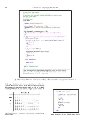
3. Proposed method
This paper presents a Three-Stage (THS) method to reach the
final solution of the UC problem. In the first stage some logical
instructions are used to produce the primal status of all unit status
in all scheduling time horizon in a matrix. It is necessary that all
committed units take some feasible and economical values (ED) in
the second stage. ED procedure in this paper follows a hybrid
artificial intelligence algorithm. PSO in series with NM when
operates on ED continues variable problem iteratively, is able to
yield an effective solution.
As it will be shown in part of simulation results, the output of
two recent stages may be considered as a suitable and near-optimal
solution in most of the time. But the final stage is still remains. The
Nomenclature
CostNH total costs of N generators in H hours;
FCi(Pih) fuel cost of ith unit with output Pih at the hth hour;
STCi Startup cost of ith unit;
Uih on/off status of ith unit; Uih ¼ 0 and Uih ¼ 1 are for
off and on statuses respectively.
N number of generators;
H number of hours;
Dh load demand at the hth hours;
Rh spinning reserve at the hth hours; spinning reserve
is the surplus power of total generation capacity
after meeting load demand at the hth hour (usually
10% of load demand)
Pi(min) minimum generation limit of the ith unit;
Pi(max) maximum generation limit of the ith unit;
MUi minimum up-time of the ith unit;
MDi minimum downtime of the ith unit;
Xi
on
duration that the ith unit is continuously on;
Xi
off
duration that the ith unit is continuously off;
(1)
Primal configuration of all
units
(A matrix with 0/1 elements for
On/Off statuses)
(3)
Solution Modification Process
(Replacing some On and Off
Statuses in each hour and
doing ED on new arrangement)
(2)
Economic Dispatch
(All nonzero statuses
take continues values)
Fig. 1. Stages of proposed method.
D (MW)
Time (h)
Variant Portion
Constant Portion
Fig. 2. A typical load demand plot. It has been divided in to constant and variant
portions.
S. Khanmohammadi et al. / Energy 35 (2010) 3072e3080 3073

3. third stage which looks for a more precise solution is called the
Solution Modification Process (SMP). This modification process
which uses some logical instructions plays the role of the local
search algorithms in AI, but acts on a single solution instead of
%h: Hour counter from 1 to Hours.
%Hours: Equals to 24 that shows time horizon in one day.
%I_hours: Is the same Initial status vector. It changes hourly with units new status.
%MU: Min Up time vector.
%MD: Min Down time vector.
%D: Demand vector.
for h=1:Hours
Commit all units with (0I_hoursMU)
while sum(Capacity of committed units)1.1*D(h)
Commit units with (I_hoursMU) one by one according to Priority Vector
end
while sum(Capacity of committed units)1.1*D(h)
Commit units with (I_hours=-MD) one by one according to Priority Vector
end
for all unchanged units so far, do as below according to reverse order of Priority Vector
if I_hours(unit)=MU(unit)
if sum(Capacity of committed units)=1.1*D(h) (20-hMD(unit) || 20-h0) *
set the unit off
else
set the unit on
end
elseif I_hours(unit)= -MU(unit)
if sum(Capacity of committed units)=1.1*D(h)
set the unit off
else
set the unit on
end
elseif I_hours(unit)0
set the unit off
end% if I_hours
end% for all unchanged units
end% for h
* In the decreasing durations of demand that committed units turn off one by one, it must be
noticed that just those units which are reachable in the next maximum of demand increasing
duration (20 in this case) are allowed to be turned off.
Fig. 3. The pseudocode of determining primal status of units. All the used data are available in the second case of study in Section 4.
Unit:
1
to
10
1 1 1 1 1 1 1 1 1 1 1 1 1 1 1 1 1 1 1 1 1 1 1 1
1 1 1 1 1 1 1 1 1 1 1 1 1 1 1 1 1 1 1 1 1 1 1 1
0 0 0 0 0 0 1 1 1 1 1 1 1 1 1 1 1 1 1 1 0 0 0 0
0 0 0 0 0 1 1 1 1 1 1 1 1 1 1 1 1 1 1 1 1 0 0 0
0 0 0 1 1 1 1 1 1 1 1 1 1 1 1 1 1 1 1 1 1 1 0 0
0 0 0 0 0 0 0 0 1 1 1 1 1 1 0 0 0 0 0 1 1 1 1 0
0 0 0 0 0 0 0 0 0 1 1 1 1 0 0 0 0 0 0 1 1 1 0 0
0 0 0 0 0 0 0 0 0 0 1 1 0 0 0 0 0 0 0 0 0 0 0 0
0 0 0 0 0 0 0 0 0 0 0 1 0 0 0 0 0 0 0 0 0 0 0 0
0 0 0 0 0 0 0 0 0 0 0 0 0 0 0 0 0 0 0 0 0 0 0 0
Hour: 1 to 24
Fig. 4. Primal arrangement of 10 unit system with 5% of spinning reserve produced by
proposed method.
% a b are tow constant.
while (Production-Demand)0.001
for i=1:a
DO PSO
end
check the convergence
for j=1:b
DO NM
end
end
Fig. 5. Pseudocode of the hybrid algorithm used for solving ED.
S. Khanmohammadi et al. / Energy 35 (2010) 3072e3080
3074

4. a population. Fig. 1; shows all the stages of the proposed method.
These stages have been described in detail as follows:
3.1. Stage one: Primal Configuration of all units
Primal Configuration of all units is based on a rule that says;
while the spinning reserve has not been satisfied, all allowable
units should be turned on according to predefined priority in any
hour of planning. It is an important notice that only those units are
allowable to be changed that satisfy the constraints (8) and (9). In
this priority, the units with large amount in their maximum
production capacity are prior to the others. At least three main
reasons can be mentioned for using such a logical priority:
i. Accessibility: because of the long MD and MU hours of big
units, it is impossible to reach them in short horizons of time.
So these units are not suitable enough to cover the hourly
changing demand. It is reasonable to use them in basic and
constant portion of hourly demand. The variant and constant
portions of demand curve have been shown in Fig. 2.
ii. Accordance: small units offer small packages of power. So this
may be so profitable to use them in the variant portion of
power demand to meet a minimum possible spinning reserve
which will impose lower cost.
iii. Economy: considering the startup cost of a big unit is more
expensive than the other units’, it is reasonable to pay this
cost primarily one time for ever. So these units will always be
on.
Since it may be found some units equal in their maximum
capacity in some UC problems, it is better to define some more
precise rules in priority determination. For example MD or MU can
be considered as a criterion. Eq. (10) is an example of priority list
that has been used in this paper. Generally, maximum capacity of
units and MD have a similar decreasing manner. The units with
larger amount in Eq. (10) are prior to other units.
Priority List ¼ PðmaxÞ;vec=maximum
n
PðmaxÞ;vec
o
þ MDvec=maximumfMDvecg (10)
The index vec presents the vector which contains related quantities
of all units. Fig. 3; shows the pseudocode of what happens in stage
one. Some values have been used in this pseudocode to make it
more understandable. These values are relevant to a ten unit
u.1 u.2 u.3 u.4 u.5 u.6 u.7 u.8 u.9 u.10
Solution1 max
P max
P max
P max
P max
P min
P min
P min
P min
P min
P
Solution2 max
P max
P max
P max
P max
P max
P max
P max
P max
P max
P
Fig. 6. Two recommended solutions for use among initial population of algorithm in solving ED.
START
1. Find the units of first
second groups in each hour.
2. Determine priority list of each group.
3. Considering
priority, { }
i
u FG
∀ ∈ do as
0
i
u =
Is h
R
satisfied?
Y
N
Find the most prior j
u { }
( )
j
u SG
∈ that has
no resemblance to i
u . If there is no
proper j
u , end the process and go to the
1
j
u =
Do the ED for the new
arrangement in this hour.
Is operating
cost
decreased?
Y
N
1
0
1
i
j
u
u
i i
=
=
= +
Accept the new arrange
go to the next hour.
END
Fig. 7. Flowchart of the solution modification process (SMP) in 1 h.
S. Khanmohammadi et al. / Energy 35 (2010) 3072e3080 3075

5. system with 10% spinning reserve. Related data are available in Case
2 of simulation results in Section 4.
A short description of the pseudocode is as follows:
a. Demand satisfying process while reaching to minimum spin-
ning reserve in each hour:
1 All committed unchangeable units (because of constraint
(9)) must remain committed.
2 Then all committed and also changeable units can remain
committed according to priority vector.
3 Finally among non committed units which are changeable,
turn units on according to priority vector.
b. For all unchanged units in each hour do as below:
1 Satisfying spinning reserve constraint (6), turn off all
allowable committed units in reverse order of priority list. It
is essential to notice that all units which turn off in
decreasing duration of demand must leave committed
before the next arriving maximum demand. Unless they can
be reachable when the demand increases. Otherwise
because of constraint (8), the power network would face
with lack of required power or required spinning reserve.
Fig. 4; Presents a typical primal arrangement of units produced
by mentioned method in less than a second.
3.2. Stage two: Economic Dispatch on primal configuration of units
As mentioned above a hybrid AI algorithm containing PSO in
series with NM is used to solve ED problem. Pseudocode of this
hybrid algorithm has been presented in Fig. 5. The PSO plus NM are
done iteratively on the ED problem to reach an error on power
balance satisfying in thousandth order as stop criterion. The
following considerations must be observed for using:
Fig. 8. Solution Modification Process (SMP) on a 10 unit system with 5% spinning reserve.
Table 1
Load demand data of 4 unit system.
Hour 1 2 3 4 5 6 7 8
Load (MW) 450 530 600 540 400 280 290 500
Table 2
Units information of 4 unit system.
Unit P(max) P(min) a b g MD MU Hsc Csc Cs hrs Initial status
(MW) (MW) ($/h) ($/MWh) ($/MW2
h) (h) (h) ($) ($) (h) (h)
1 300 75 648.74 16.83 0.0021 5 4 500 1100 5 8
2 250 60 585.62 16.95 0.0042 5 3 170 400 5 8
3 80 25 213.00 20.74 0.0018 4 2 150 350 4 5
4 60 20 252.00 23.60 0.0034 1 1 0 0.02 0 6
S. Khanmohammadi et al. / Energy 35 (2010) 3072e3080
3076

6. i. Because of the non-perfect successful rate of AI algorithms in
finding the optimal solution, it is recommended to repeat the
algorithm at most six times. However after four runs that
improvement occurs, the repetition can be stopped.
ii. Merging a calculated solution by random initial population of
algorithm may accelerate the convergence of the algorithm.
As we know because of common small amounts of spinning
reserve (5e10%), it is predictable that all of the committed
units have to work in near around their full capacitance.
Knowing this point, Fig. 6 describes more about how to create
such solutions in a 10 unit system.
iii. The bad convergence of solutions must be checked between
PSO and NM to prevent useless extra cost evaluations. This
causes to save considerable amount of time.
iv. Whereas the dimension of ED problems changes by number
of committed units in each hour, they have not the same
complexity. To save much more execution time, we can use
different population size in each hour. The recommended
population size for PSO is usually a constant value between 20
and 50. But in this paper an hourly changing population size is
used as follows:
Npopulation;h ¼ a þ 3ðn:c:uÞh (11)
When Npopulation,h is the population size in hth hour, a ˛
{20,21,.40}, 3 ˛ {1,2} and (n.c.u)h is the number of committed units
in hth hour.
3.3. Stage three: Solution Modification Process (SMP)
The solution produced by two stages is near optimal, but this part
introduces a modificationprocess that yields a more precise solution
by acting on the produced solution. Considering constraints (8) and
(9), any replacement in solution elements may cause in its dis-
assembling. The proposed SMP devises a plan to decrease the cost by
saving the total shape of solution while satisfying two mentioned
constraints. In brief, just those units that do not take any affect in the
other hours are allowed to be changed their status.
The procedure is as follows:
i. Determine all units in each hour which are allowed to be
turned off as the first group (FG).
ii. Then in the same hour, determine the second group (SG) with
units that are allowed to be committed instead of the units
belong to FG.
iii. In this step, it is needed to replace the units belonging to the
FG with the units belonging to the SG one by one. After doing
ED on the new arrangement, if the operating cost of this hour
has been decreased, it will be preferred to the primary
arrangement. Some units are prior to the others in both
groups to commence the replacements. Those units which
have more expensive operating constant cost (a) are prior to
the other units in the FG. The priority list of units which
belong to SG is defined as Eq. (12). The units with lower
amounts are prior to the others.
Priority List ¼ Diffrence of STCis in new and old status of units
þ avec
(12)
Fig. 7; describes the SMP in more detail.
Considering second note on stage two, the recent ED solution of
each hour can be merged by the random initial population instead
of those were showed in Fig. 6. This solution accelerates the
searching process of ED in the third stage. Fig. 8; depicts how the
SMP acts on output of two latest stages. Five modifications have
been done on primary configuration. Rectangular and oval boxes
present the units of FG and SG respectively. The other on/off units in
the same hours are those which are not allowable to be changed.
4. Simulation results
In this section we are going to test the efficiency of the proposed
method by solving some standard UC problems. These standard
problems contain four unit systems, two versions of ten unit system
and twenty unit systems. The last column of data tables of units in
each system contains the information of initial status of units. The
Table 3
Simulation results of 4 unit system. B.SMP and A.SMP are the amounts for before and
after SMP respectively. Sign (e) means that no amount has been reported.
Method Best ($) Average ($) Worst ($)
LR [19] 75232 e e
PSOeLR [19] 74808 e e
Proposed B. SMP 74812 74877 75166
A. SMP 74812 74877 75166
Table 4
Load demand data of 10 unit system.
Hour 1 2 3 4 5 6 7 8 9 10 11 12
Load (MW) 700 750 850 950 1000 1100 1150 1200 1300 1400 1450 1500
Hour 13 14 15 16 17 18 19 20 21 22 23 24
Load (MW) 1400 1300 1200 1050 1000 1100 1200 1400 1300 1100 900 900
Table 5
Units information of 10 unit system.
Unit P(max) P(min) a b g MD MU Hsc Csc Cs hrs Initial status
(MW) (MW) ($/h) ($/MWh) ($/MW2
h) (h) (h) ($) ($) (h) (h)
1 455 150 1000 16.19 0.00048 8 8 4500 9000 5 8
2 455 150 970 17.26 0.00031 8 8 5000 10000 5 8
3 130 20 700 16.60 0.002 5 5 550 1100 4 5
4 130 20 680 16.50 0.00211 5 5 560 1120 4 5
5 162 25 450 19.70 0.00398 6 6 900 1800 4 6
6 80 20 370 22.26 0.00712 3 3 170 340 2 3
7 85 25 480 27.74 0.0079 3 3 260 520 2 3
8 55 10 660 25.92 0.00413 1 1 30 60 0 1
9 55 10 665 27.27 0.00222 1 1 30 60 0 1
10 55 10 670 27.92 0.00173 1 1 30 60 0 1
S. Khanmohammadi et al. / Energy 35 (2010) 3072e3080 3077

7. negative and positive amounts show the hours the units were off
and on respectively before the first hour. Results of the proposed
method have two parts: Simulation results before SMP and after
SMP. This gives a better comparison of SMP abilities. Also three
different fonts have been used in tables of simulation results: the
lowest cost in each column is shown in Bold. The other reported
methods which present a more expensive cost in respect of
proposed method have been shown in italic. The rest amounts have
been shown by ordinary font. The best, average and the worst
amounts have been yielded after several executions of presented
methods. In this paper 10 runs have been executed for proposed
method.
Case 1: This system contains four power generating units. Load
demand data is shown in Table 1. As it is clear, the time horizon of
this problem is 8 h. Table 2, presents the data of this four unit
system. As it can be seen in Table 3, the proposed method is the best
method after the PSOeLR [19] with just four dollars difference.
Another important index of a good solution is robustness of the
method over several executions. The methods that yield similar
solutions in various executions are more reliable than the other
methods. The low average amount of THS confirms its robustness.
Case 2: A system with ten generating units has been selected to
study in this part. Table 4 contains the information of load demand
in 24 h. This system has two very usual UC problems. Ten unit
system with 5% spinning reserve and ten unit system with 10%
spinning reserve. Here we are going to solve this system with 5% of
spinning reserve and the next one will be considered in the third
case. Table 5 yields more information of these ten units.
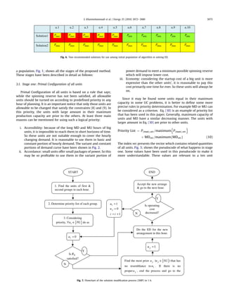
Remarkable results of proposed method are seen in Table 6. THS
presents the lowest costs in all three Best, Average and Worst
columns. Also as mentioned above, the low average amount
emphasizes on robustness of THS method. Arrangement of units in
all 24 h of a day after SMP is shown in Fig. 9. Fuel cost, startup cost
and modification rate after SMP are presented respectively in three
right columns.
Case 3: The same units mentioned in case 2 but with 10%
spinning reserve. Table 7 compares the reported methods. THS
surpasses other methods in Best and Worst amounts. The average
amounts show that THS has the third rank after AG [30] and
CReGA [31].
Case 4: By duplicating the amounts of Case 2, it is possible to
define a new UC problem with 20 units. This problem has been
known as a standard UC problem. Presence of many similar units
in a UC problem may challenge the methods in choosing one
situation among many possible situations. These kinds of problem
may have some optimum solutions with equal costs. Table 8,
contains results of proposed method and some other method. In
column of Best costs just EALR [12] has lower cost than proposed
method. However most of the average and worst amounts has not
been reported, but the proposed method includes the enough
efficiency to yield suitable costs with respect to most of the other
methods.
Table 6
Simulation results of 10 unit system with 5% of spinning reserve. B.SMP and A.SMP
are the amounts for before and after SMP respectively. Sign (e) means that no
amount has been reported.
Method Best ($) Average ($) Worst ($)
BPSO [20] 565,804 566,992 567,251
GA [20] 570,781 574,280 576,791
APSO [21] 561,586 e e
BP [21] 565,450 e e
TSGB [22] 560,263.9151 e e
IPSO [23] 558,114.8 e e
Hybrid PSOeSQP
[24]
568,032.3 e e
Proposed B.SMP 558,844.7568 558,937.2371 559,154.9755
A.SMP 557,676.8104 557,769.2891 557,987.0291
Modification Rate
($)
Start up cost
($)
Fuel Cost
($)
10
9
8
7
6
5
4
3
2
1
Unit
0
0
13684
0
0
0
0
0
0
0
0
245
455
H01
0
0
14554
0
0
0
0
0
0
0
0
295
455
H02
0
0
16302
0
0
0
0
0
0
0
0
395
455
H03
0
900
18598
0
0
0
0
0
40
0
0
455
455
H04
0
0
19609
0
0
0
0
0
90
0
0
455
455
H05
31.1440
560
21860
0
0
0
0
0
60
130
0
455
455
H06
0
1100
23262
0
0
0
0
0
25
130
130
410
455
H07
0
0
24150
0
0
0
0
0
30
130
130
455
455
H08
253.1673
340
26589
0
0
0
0
20
110
130
130
455
455
H09
0
520
29336
0
0
0
25
43
162
130
130
455
455
H10
0
60
31220
0
0
13
25
80
162
130
130
455
455
H11
0
60
33205
0
10
53
25
80
162
130
130
455
455
H12
0
0
29336
0
0
0
25
43
162
130
130
455
455
H13
253.1673
0
26589
0
0
0
0
20
110
130
130
455
455
H14
0
0
24150
0
0
0
0
0
30
130
130
455
455
H15
0
0
21514
0
0
0
0
0
25
130
130
310
455
H16
0
0
20642
0
0
0
0
0
25
130
130
260
455
H17
0
0
22387
0
0
0
0
0
25
130
130
360
455
H18
0
0
24150
0
0
0
0
0
30
130
130
455
455
H19
0
600
29336
0
0
0
25
43
162
130
130
455
455
H20
31.1410
0
27267
0
0
0
25
73
162
130
0
455
455
H21
0
0
22735
0
0
0
25
20
145
0
0
455
455
H22
39.3298
0
17645
0
0
0
0
20
0
0
0
425
455
H23
0
0
15427
0
0
0
0
0
0
0
0
345
455
H24
4140
553540
Total Cost ($)= 557677
Fig. 9. Solution of 10 generating unit with 5% of spinning reserve, presented by proposed method. Some amounts may have round off error.
S. Khanmohammadi et al. / Energy 35 (2010) 3072e3080
3078

8. 5. Conclusion
In this paper by presentation of a new three-stage method
(THS), some of widely used and standard problems of UC were
solved and were compared with several other methods. The
proposed method gains from some logical and simple steps
combined with an intelligent algorithm. THS produces primal on/
off status of the all units during all planning horizon. Then does ED
and finally via a novel solution modification process (SMP) modifies
the initially produced schedule and yields a schedule with
comparable total cost including fuel and startup costs. Simulation
results confirm that THS is more economical than many other
methods and its solutions are considerably robust and reliable over
several executions.
Applying the THS to the large-scale UC problems and also doing
some supplementary improvements on its procedure can be the
subject of future researches.
Acknowledgment
The authors would like to thank their dear friend Ehsan Bathaei
from the Royal Melbourne Institute of Technology (RMIT) for the
revision of this paper.
References
[1] Saber AY. Scalable unit commitment by memory bounded ant colony opti-
mization with A* local search. Electrical Power Energy Systems 2008;30
(6e7):403e14.
[2] Hossein SH, Khodaei A, Aminifar F. A novel straightforward unit commitment
method for large-scale power systems. IEEE Transactions on Power Systems
2007;22(4):2134e43.
[3] Wood AJ, Wollenberg FB. Power generation operation and control. 2nd ed.
New York: Wiley-Interscience; 1996.
[4] Kerr RH, Scheidt JL, Fontana AJ, Wiley JK. Unit commitment. IEEE Transactions
on Power Apparatus and Systems 1966;85(5):417e21.
[5] Bums RM, Gibson CA. Optimization of priority lists for a unit commitment
program. In: Proceedings of the IEEE power engineering society summer
meeting; 1975.
[6] Lee FN. Short-term thermal unit commitment- a new method. IEEE Trans-
actions on Power Systems 1998;3(2):421e8.
[7] Senjyu T, Shimabukuro K, Uezato K, Funabashi T. A fast technique for unit
commitment problem by extended priority list. IEEE Transactions on Power
Systems 2003;18(2):882e8.
[8] Lowery PG. Generating unit commitment by dynamic programming. IEEE
Transactions on Power Apparatus and Systems 1996;85(5):422e6.
[9] Happ HH, Johnson RC, Wright WJ. Large scale hydro-thermal unit commit-
ment-method and results. IEEE Transactions on Power Apparatus and Systems
1971;90(3):1373e84.
[10] Merlin A, Sandrin P. A method for unit commitment at Electricite de France.
IEEE Transactions on Power Apparatus and Systems 1983;102(5):1218e25.
[11] Aoki K, Itoh M, Satoh T, Nara K, Kanezashi M. Optimal long-term Unit
Commitment in large scale systems including fuel constrained thermal and
pumped-storage hydro. IEEE Transactions on Power Systems 1989;4
(3):1065e73.
[12] Ongsakul W, Petcharaks N. Unit Commitment by enhanced adaptive
Lagrangian relaxation. IEEE Transactions ion Power Systems 2004;19
(1):620e8.
[13] Kazarlis SA, Bakirtzis AG, Petridis V. A genetic algorithm solution to the unit
commitment problem. IEEE Transactions on Power Systems 1996;11
(1):83e92.
[14] Mantawy AH, Abdel-Magid YL, Selim SZ. A simulated annealing algorithm for
unit commitment. IEEE Transactions on Power Systems 1998;13(1):197e204.
[15] Mori H, Matsuzaki O. Application of priority-list-embeded tabu search to unit
commitment in power systems. Transactions of the Institute of Electrical
Engineers of Japan 2001;121-B(4):535e41.
[16] Ting TO, Rao MVC, Loo CK. A novel approach for unit commitment problem via
an effective hybrid particl sowarm optimization. IEEE Transactions on Power
Systems 2006;21(1):411e8.
[17] Kennedy J, Eberhart RC. Particle swarm optimization. In: Proceedings of IEEE
international conference on neural network, vol. 2. Piscataway, NJ: IEEE
Service Center; 1995. p. 1942e8.
[18] Lagarias JC, Reeds JA, Wright MH, Wright PE. Convergence properties of the
Nelder Mead simplex method in low dimensions. Journal of the Society for
Industrial and Applied Mathematics 1998;9(1):112e47.
[19] Sriyanyong P, Song YH. Unit commitment using particle swarm optimization
combined with Lagrange relaxation. In: Power Engineering Society general
meeting, vol. 3; 2005. p. 2752e9.
[20] Gaing ZL. Discrete particle swarm optimization algorithm for unit commit-
ment. In: IEEE Power Engineering Society general meeting, vol. 1; 2003. p.
13e7.
[21] Pappala VS, Erlich I. A new approach for solving the unit commitment
problem by adaptive particle swarm optimization, Power and Energy Society
general meeting-conversion and delivery of electrical energy in the 21st
century. USA: IEEE; 2008. p. 1e6.
[22] Eldin AS, El-sayed MAH, Youssef HKM. A two-stage genetic based technique
for the unit commitment optimization problem. In: 12th International Middle
East Power System Conference, MEPCO, Aswan; 2008. p. 425e30.
[23] Xiong W, Li MJ, Cheng YL. An improved particle swarm optimization algo-
rithm for unit commitment. In: Proceedings of the 2008 international
conference on intelligent computation technology and automation, vol. 01;
2008. p. 21e5.
[24] Victoire TAA, Jeyakumar AE. Hybrid PSOSQP for economic dispatch with
valve-point effect. Electric Power Systems Research 2004;71(1):51e9.
[25] Juste KA, Kita H, Tunaka E, Hasegawa J. An evolutionary programming solution
to the unit commitment problem. IEEE Transactions on Power Systems
1999;14(4):1452e9.
[26] Senjyu T, Yamashiro H, Uezato K, Funabashi T. A unit commitment problem by
using genetic algorithm based on unit characteristic classification. In:
Proceedings of the IEEE Power Engineering Society winter meeting, vol. 1;
2002. p. 58e63.
[27] Cheng CP, Liu CW, Liu CC. Unit commitment by Lagrangian relaxation and
genetic algorithms. IEEE Transactions on Power Systems 2000;15
(2):707e14.
[28] Chusanapiputt S, Nualhong D, Jantarang S, Phoomvuthisarn S. A Solution to
unit commitment problem using hybrid ant system/priority list method. In:
IEEE 2nd international conference on power and energy, PECon 08, Malaysia;
2008. p. 1183e8.
Table 7
Simulation results of 10 unit system with 10% of spinning reserve. B.SMP and A.SMP
are the amounts for before and after SMP respectively. Sign (e) means that no
amount has been reported.
Method Best ($) Average ($) Worst ($)
EP [25] e 565,352 e
GA [13] 565,852 e 570,032
UCCeGA [26] 563,977 e 565,606
DP [13] 565,825 e e
LR [13] 565,825 e e
LRGA [27] 564,800 e e
HPSO [16] 563,942.3 564,772.3 565,782.3
HASP [28] 564,029 564,324 564,490
ICGA [29] e 566,404 e
AG [30] e 564,005 e
EALR [12] 563,977 e e
CReGA [31] e 563,977 e
MPL [32] 563,977.1 e e
TSGB [22] 568,315 e e
Proposed B.SMP 564,017.73 564,121.46 564,401.08
A.SMP 563,937.26 564,040.30 64,320.61
Table 8
Simulation results of 20 unit system with 10% of spinning reserve. B.SMP and A.SMP
are the amounts for before and after SMP respectively. Sign (e) means that no
amount has been reported.
Method Best ($) Average ($) Worst ($)
ICGA [29] e 1,127,244 e
LRGA [27] e 1,122,622 e
GA [13] 1,126,243 e 1,132,059
LR [13] 1,130,660 e e
EP [25] 1,125,494 1,127,257 1,129,793
AG [30] e 1,124,651 e
BCGA [29] 1,130,291 e e
UCCeGA [26] 1,125,516 e e
DPLR [12] 1,128,098 e e
SF [2] 1,125,161 e e
EALR [12] 1,123,297 e e
CReGA [31] e 1,236,981 e
Proposed B.SMP 1,124,838 1,125,102 1,125,283
A.SMP 1124490 1,124,803 1,124,995
S. Khanmohammadi et al. / Energy 35 (2010) 3072e3080 3079

9. [29] Damousis IG, Bakirtzis AG, Dokopoulos PS. A solution to the unit commitment
problem using integer-coded genetic algorithm. IEEE Transactions on Power
Systems 2004;19(2):1165e72.
[30] Satoh T, Nara K. Maintenance scheduling by using simulated annealing
method for power plants. IEEE Transactions on Power Systems 1991;6
(2):850e7.
[31] Tokoro KI,MasudaY,Nishina H.Solvingunit commitmentproblem bycombining
of continuous relaxation method and genetic algorithm. In: SICE annual
conference. Japan: The University Electro-Communications; 2008. p. 3474e8.
[32] Tingfang Y, Ting TO. Methodological priority list for unit commitment
problem. In: International conference on computer science and software
engineering, CSSE, vol. 1; 2008. p. 176e9.
S. Khanmohammadi et al. / Energy 35 (2010) 3072e3080
3080