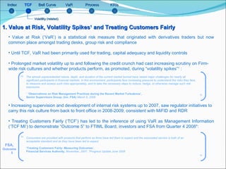
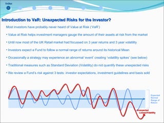
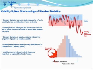
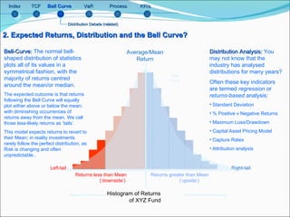
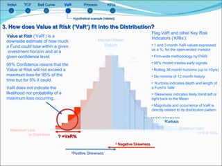
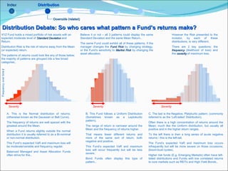
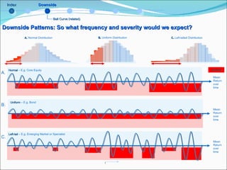
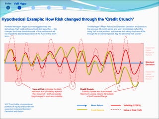
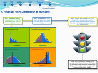
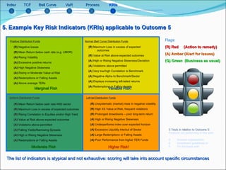
Treating Customers Fairly Technical Guide to Value at Risk, Key Risk Indicators and Logic Tests by Jon Beckett, BA, ASI,  For the CCC Introduction Index
Bell Curve Index TCF VaR Process KRIs 1. Value at Risk, Volatility Spikes 1  and Treating Customers Fairly Value at Risk (‘VaR’) is a statistical risk measure that originated with derivatives traders but now common place amongst trading desks, group risk and compliance Until TCF, VaR had been primarily used for trading, capital adequacy and liquidity controls Prolonged market volatility up to and following the credit crunch had cast increasing scrutiny on Firm-wide risk cultures and whether products perform, as promoted, during “volatility spikes” 1  :   Increasing supervision and development of internal risk systems up to 2007, saw regulator initiatives to carry this risk culture from back to front office in 2008-2009, consistent with MiFID and RDR Treating Customers Fairly (‘TCF’) has led to the inference of using VaR as Management Information (‘TCF MI’) to demonstrate “Outcome 5” to FTIML Board, investors and FSA from Quarter 4 2008*:  FSA,  Outcome  5 The almost unprecedented nature, depth, and duration of the current market turmoil have raised major challenges for nearly all significant participants in financial markets. In this environment, participants face increasing pressure to understand the risks they face, to measure and assess such risks appropriately, and to take the necessary steps to reduce, hedge, or otherwise manage such risk exposures. 1   ‘Observations on Risk Management Practices during the Recent Market Turbulence’,  Senior Supervisors Group; (inc. FSA)  March 6, 2008 Consumers are provided with products that perform as firms have led them to expect and the associated service is both of an acceptable standard and as they have been led to expect  ‘ Treating Customers Fairly: Measuring Outcomes’,  Financial Services Authority,  November, 2007, *Progress Update June 2008 Volatility (related) “ ” ” “
Index Introduction to VaR: Unexpected Risks for the Investor? Most investors have probably never heard of Value at Risk (‘VaR’) Value at Risk helps investment managers gauge the amount of their assets at risk from the market Until now most of the UK Retail market had focussed on 3 year returns and 3 year volatility Investors expect a Fund to follow a normal range of returns around its historical Mean Occasionally a strategy may experience an abnormal ‘event’ creating ‘volatility spikes’ (see below) Traditional measures such as Standard Deviation (Volatility) do not quantify these unexpected risks We review a Fund’s  risk  against 3 tests: investor expectations, investment guidelines and basis sold Unexpected  Losses/Volatility Expected Normal Range of Return
Index What is Volatility: What does Standard Deviation tell us about a Fund? Standard Deviation measures the volatility of a Fund’s returns around the Mean Return  The Mean Return is the average return over a specific period – think of it as the thick centre line on the chart right Standard Deviation is the moving line above and below the centre Mean Return line, we call this ‘dispersion’ Standard Deviation is normally considered more reliable over longer time periods; (such as 3 or 5 years) using monthly returns The volatility of returns can also be shown in a histogram of returns (right) – the greater the frequency of returns away from the Mean the higher the Volatility Fund XYZ Returns over 36 Months Standard Deviation   (‘Volatility’)  Negative Deviation Positive Deviation Mean  Return Up Down Volatility Spikes (related) Volatility
Index Volatility Spikes: Shortcomings of Standard Deviation Standard Deviation is a good single measure for a Fund’s Volatility but can be misleading in terms of all risks Volatility does not actually tell you how much a Fund has lost or gained; simply how volatile its returns were between two points Standard Deviation, in isolation, does not indicate the proportion of positive or negative volatility Volatility alone does not reliably convey short-term risk or changes in risk (‘volatility spikes’) Volatility does not indicate the likely frequency, magnitude or expected likelihood of losses Standard Deviation   =  (Expected Risk) ? Normal Volatility Volatility Spike: Unexpected Risk? Hypothetical example (related) Vol. Spikes Unexpected Risk? ?
Average/Mean Return Bell Curve Bell Curve Index TCF VaR Process KRIs 2. Expected Returns, Distribution and the Bell Curve? Histogram of Returns  of XYZ Fund Left-tail Returns less than Mean  (‘downside’) Bell-Curve:  The normal bell-shaped distribution of statistics plots all of its values in a symmetrical fashion, with the majority of returns centred around the mean/or median.  The expected outcome is that returns following the Bell Curve will equally plot either above or below the mean; with diminishing occurrences of returns away from the mean. We call those less-likely returns as ‘tails’.  This model expects returns to revert to their Mean; in reality investments rarely follow the perfect distribution, as Risk is changing and often unpredictable..  Returns greater than Mean  (‘upside’) Right-tail Distribution Analysis:  You may not know that the industry has analysed distributions for many years?  Often these key indicators are termed  regression  or  returns-based  analysis: Standard Deviation % Positive v Negative Returns Maximum Loss/Drawdown Capital Asset Pricing Model  Capture Rates Attribution analysis Distribution Debate (related)
Bell Curve Index TCF VaR Process KRIs Maximum Loss  or Drawdown Median/Mean Return Bell Curve Value at Risk  (‘VaR’) is a downside estimate of how much a Fund could lose within a given  investment horizon and at a given confidence level. 95% Confidence means that the Value at Risk will not exceed a maximum loss for 95% of the time but for 5% it could.  VaR does not indicate the likelihood nor probability of a maximum loss occurring.. Flag VaR and other Key Risk Indicators (‘KRIs’): 1 and 3 month VaR values expressed as a %, for the open-ended investor Firm-wide methodology by PAIR 95% model creates early signals Rolling 36 month horizons (up to 10yrs) De minimis of 12 month history  1 Kurtosis indicates depth and length of a Fund’s ‘tails’  2 Skewness indicates likely trend left or right back to the Mean Magnitude and occurrence of VaR is directly related to its distribution pattern  1 Kurtosis Maximum Gain  or Bull Rally 2 Positive Skewness 2  Negative Skewness 3. How does Value at Risk (‘VaR’) fit into the Distribution? Hypothetical example (related) ? =VaR%
Index Distribution Debate: So who cares what pattern a Fund’s returns make? Distribution XYZ Fund holds a mixed portfolio of risk assets with an expected moderate level of  Standard Deviation  and Return.  Distribution Risk is the risk of returns away from the Mean (or expected) return. The patterns of returns could look like any of those below; the majority of patterns are grouped into a few broad categories.. Downside (related) Believe it or not – all 3 patterns could display the same Standard Deviation and the same Mean Return.. The same Fund could exhibit all of these patterns, if the manager changes the  Fund Risk  by changing strategy, or the Fund’s sensitivity to  Market Risk  by changing the asset allocation. However the Risk presented to the investor, by each of these distributions, is very different.  There are 2 key questions: the  frequency  (likelihood of loss) and the  severity  of maximum loss. A. This is the Normal distribution of returns; (otherwise known as the Gaussian or Bell Curve). The frequency of returns are well spaced with the greatest around the Mean.  When a Fund returns slightly outside the normal distribution it is usually referred to as a Bi-nominal or non-normal distribution.  This Fund’s expected VaR and maximum loss will be moderate/variable and frequency regular. Balanced Managed and Asset Allocation Funds often strive for this..  B. This Fund follows a Uniform Distribution (Sometimes known as a Leptokurtic pattern). The range of return is narrower around the Mean and the frequency of returns higher.  That means fewer different returns and more of the same sort of return, both negative and positive. This Fund’s expected VaR and maximum loss will occur frequently but will be less severe.  Bond Funds often display this type of pattern.. C. The last is the Negative, Platykurtic pattern; (commonly referred to as the ‘Left-tailed’ Distribution). Often there is a high concentration of returns around the Mean; much like the Uniform distribution, but usually all positive and in the higher return ranges. To the left there is then a long series of acute negative returns - this is the left-tail. The Fund’s expected VaR and maximum loss occurs infrequently but will be more severe on those occasions; (boom-bust cycles). Higher risk funds (E.g. Emerging Markets) often have left-tailed distributions and Funds with low correlated returns to core markets such as REITs and High Yield Bonds.. Frequency over time  t Severity Severity Severity
Index Downside Patterns: So what frequency and severity would we expect? Downside Bell Curve (related) A.  Normal Distribution B.  Uniform Distribution C.  Left-tailed Distribution Mean  Return over time Mean  Return over time Mean  Return over time Normal  – E.g. Core Equity Volatility t B. Uniform  – E.g. Bond A. C. Left-tail  – E.g. Emerging Market or Specialist
Index Hypothetical Example: How Risk changed through the ‘Credit Crunch’ Credit Crunch:   Volatility Spikes lead to increased Maximum Losses, returns fall outside of the Expected Range Expected Upper Range of Return Standard Deviation Expected Lower Range of Return VaR Hypo XYZ Fund holds a conventional portfolio of equity and bonds with expected moderate Standard Deviation and Return The Manager’s Mean Return and Standard Deviation are based on the previous 36 month period and won’t immediately reflect the rising VaR in the portfolio. VaR values and rolling short-term KRIs, through the investment period, flag the abnormal risk sooner! Mean Return Value at Risk:  indicates the likely maximum size of volatility spikes if they occurred – VaR can quickly flag changes in short-term volatility Fund Returns Volatility (STDEV) Value at Risk (VaR) Portfolio Managers began to invest aggressively into derivatives, high yield and securitised debt securities – this changed the future distribution/risk of the portfolio but will not impact the Standard Deviation of the Fund in the short-term..
Bell Curve Index TCF VaR Process KRIs 4. Process: From Distribution to Outcome  Step1. PAIR Stress-testing  –Indices/Sectors are tested for historical indicators once per annum Step2. Fund Patterns  – PAIR test ongoing data and supply fund level reports on a regular basis Left-tail Distribution Funds Positive Distribution Funds Uniform Distribution Funds Normal (Bell Curve) Distribution Funds Marginal Risk Variable Risk! Moderate Risk Higher Risk! Step3. Analysis of Outcomes –  Designated Manager, or analyst, analyses Key Risk Indicators (‘KRIs’) against expected outcomes from Step1. Set of logical tests are applied for each distribution type Step4. Flag Outcomes and Actions –  Score funds as either ‘Green’, ‘Amber’ or ‘Red’ based on Step3 and prepare the health monitor report for peer review and escalates alerts or action through Global Product Strategy. Framework (related)
Bell Curve Index TCF VaR Process KRIs 5. Example Key Risk Indicators (KRIs) applicable to Outcome 5 The list of indicators is atypical and not exhaustive: scoring will take into account specific circumstances (R)  Negative losses  (R)  Mean Return below cash rate (e.g. LIBOR) (A)  Rising Volatility (A)  Excessive positive returns (A)  High Negative Skewness (A)  Rising or Moderate Value at Risk (A)  Redemptions or Falling Assets (A)  Above average TERs ( R)  Mean Return below cash rate AND sector (R)  Maximum Loss in excess of expected outcomes  (R)  Rising Correlation to Equities and/or High Yield (A)  Value at Risk above expected outcomes  (A)  Violations above permitted (A)  Falling Yields/Narrowing Spreads (A)  High or Rising Negative Skewness (A)  Redemptions or Falling Assets (R)  Maximum Loss in excess of expected outcomes  (R)  Value at Risk above expected outcomes  (A)  High or Rising Negative Skewness/Deviation (A)  Violations above permitted (A)  Very low/high Correlation to Benchmark (A)  Negative Alpha to Benchmark/Sector (A)  Displays increasing left-tailed returns (A)  Redemptions or Falling Assets (R)  Unsystematic (market) rises in negative volatility (R)  High XS Value at Risk, frequent violations (R)  Prolonged drawdowns – poor long-term return (A)  High or Rising Negative Skewness (A)  Underperforms index over expected horizon (A)  Excessive Liquidity into/out of Sector (A)  Large Redemptions or Falling Assets (A)  Poor Performance from higher TER Funds Flags: (R) Red  (Action to remedy) (A) Amber (Alert for issues) (G) Green  (Business as usual) 3 Tests in relation to Outcome 5:   Products not performing in line with:  Investor expectations Investment guidelines or  On the basis sold Left-tail Distribution Funds Uniform Distribution Funds Marginal Risk Variable Risk! Moderate Risk Higher Risk! Positive Distribution Funds Normal (Bell Curve) Distribution Funds
Value at Risk Factor =   Normal Distribution   Confidence Level; E.g. 95% (1.96) Standard deviation of historical fund returns. = The number of months (36) or days (20) measured Value at Risk Amount = VaR Factor * NAV NAV = Net Asset Value of the Fund Value at Risk  (‘VaR’) is a downside estimate of how much a Fund could lose within a given investment horizon and at a given confidence level. 95% Confidence means that the Value at Risk will not exceed a maximum loss for 95% of the time but for 5% it could. VaR does not indicate the likelihood nor probability of a maximum loss occurring..
Confidence % ( Intervals) = About 68% of values in a normal distribution are within one standard deviation (sigma, σ) away from the Mean (μ); about 95% of the values are within two standard deviations and about 99.7% lie within three standard deviations. Each standard deviation multiple (sigma , σ) then provides confidence intervals of expected ranges of return. To be more precise, the area under the bell curve between Mean and +/− each sigma multiple (σ) in terms of the cumulative normal distribution function is given by the error function (erf). To 12 decimal places, the 1 to 6 sigma multiples are: You can then reverse the relation of sigma multiples for a few associated indicators used to describe the area under the bell curve. These values are useful to determine (asymptotic) confidence intervals for other indicators based on a normally distributed curve. The sigma multiples and confidence intervals are shown right. The left table then indicates the proportion (Confidence%) of a given interval and n is a multiple of the standard deviation that specifies the width of each interval. 4.4172 0.99999 3.8906 0.9999 3.29052 0.999 3.09023 0.998 2.80703 0.995 2.57583 0.99 2.32635 0.98 1.95996 0.95 1.64485 0.90   1.28155  0.80 Interval Width (n) 68% 99.999% 99.99% 99,9% 99.8% 99.5% 99% 98% 95% 90% 80% Confidence% 0.999999998027 6 0.999999426697 5 0.999936657516 4 0.997300203937 3 0.954499736104 2   0.682689492137  1 σ Interval

Intro To VaR, Distributions, KRIs And Logic Test

  • 1.
    Treating Customers FairlyTechnical Guide to Value at Risk, Key Risk Indicators and Logic Tests by Jon Beckett, BA, ASI, For the CCC Introduction Index
  • 2.
    Bell Curve IndexTCF VaR Process KRIs 1. Value at Risk, Volatility Spikes 1 and Treating Customers Fairly Value at Risk (‘VaR’) is a statistical risk measure that originated with derivatives traders but now common place amongst trading desks, group risk and compliance Until TCF, VaR had been primarily used for trading, capital adequacy and liquidity controls Prolonged market volatility up to and following the credit crunch had cast increasing scrutiny on Firm-wide risk cultures and whether products perform, as promoted, during “volatility spikes” 1 : Increasing supervision and development of internal risk systems up to 2007, saw regulator initiatives to carry this risk culture from back to front office in 2008-2009, consistent with MiFID and RDR Treating Customers Fairly (‘TCF’) has led to the inference of using VaR as Management Information (‘TCF MI’) to demonstrate “Outcome 5” to FTIML Board, investors and FSA from Quarter 4 2008*: FSA, Outcome 5 The almost unprecedented nature, depth, and duration of the current market turmoil have raised major challenges for nearly all significant participants in financial markets. In this environment, participants face increasing pressure to understand the risks they face, to measure and assess such risks appropriately, and to take the necessary steps to reduce, hedge, or otherwise manage such risk exposures. 1 ‘Observations on Risk Management Practices during the Recent Market Turbulence’, Senior Supervisors Group; (inc. FSA) March 6, 2008 Consumers are provided with products that perform as firms have led them to expect and the associated service is both of an acceptable standard and as they have been led to expect ‘ Treating Customers Fairly: Measuring Outcomes’, Financial Services Authority, November, 2007, *Progress Update June 2008 Volatility (related) “ ” ” “
  • 3.
    Index Introduction toVaR: Unexpected Risks for the Investor? Most investors have probably never heard of Value at Risk (‘VaR’) Value at Risk helps investment managers gauge the amount of their assets at risk from the market Until now most of the UK Retail market had focussed on 3 year returns and 3 year volatility Investors expect a Fund to follow a normal range of returns around its historical Mean Occasionally a strategy may experience an abnormal ‘event’ creating ‘volatility spikes’ (see below) Traditional measures such as Standard Deviation (Volatility) do not quantify these unexpected risks We review a Fund’s risk against 3 tests: investor expectations, investment guidelines and basis sold Unexpected Losses/Volatility Expected Normal Range of Return
  • 4.
    Index What isVolatility: What does Standard Deviation tell us about a Fund? Standard Deviation measures the volatility of a Fund’s returns around the Mean Return The Mean Return is the average return over a specific period – think of it as the thick centre line on the chart right Standard Deviation is the moving line above and below the centre Mean Return line, we call this ‘dispersion’ Standard Deviation is normally considered more reliable over longer time periods; (such as 3 or 5 years) using monthly returns The volatility of returns can also be shown in a histogram of returns (right) – the greater the frequency of returns away from the Mean the higher the Volatility Fund XYZ Returns over 36 Months Standard Deviation (‘Volatility’) Negative Deviation Positive Deviation Mean Return Up Down Volatility Spikes (related) Volatility
  • 5.
    Index Volatility Spikes:Shortcomings of Standard Deviation Standard Deviation is a good single measure for a Fund’s Volatility but can be misleading in terms of all risks Volatility does not actually tell you how much a Fund has lost or gained; simply how volatile its returns were between two points Standard Deviation, in isolation, does not indicate the proportion of positive or negative volatility Volatility alone does not reliably convey short-term risk or changes in risk (‘volatility spikes’) Volatility does not indicate the likely frequency, magnitude or expected likelihood of losses Standard Deviation = (Expected Risk) ? Normal Volatility Volatility Spike: Unexpected Risk? Hypothetical example (related) Vol. Spikes Unexpected Risk? ?
  • 6.
    Average/Mean Return BellCurve Bell Curve Index TCF VaR Process KRIs 2. Expected Returns, Distribution and the Bell Curve? Histogram of Returns of XYZ Fund Left-tail Returns less than Mean (‘downside’) Bell-Curve: The normal bell-shaped distribution of statistics plots all of its values in a symmetrical fashion, with the majority of returns centred around the mean/or median. The expected outcome is that returns following the Bell Curve will equally plot either above or below the mean; with diminishing occurrences of returns away from the mean. We call those less-likely returns as ‘tails’. This model expects returns to revert to their Mean; in reality investments rarely follow the perfect distribution, as Risk is changing and often unpredictable.. Returns greater than Mean (‘upside’) Right-tail Distribution Analysis: You may not know that the industry has analysed distributions for many years? Often these key indicators are termed regression or returns-based analysis: Standard Deviation % Positive v Negative Returns Maximum Loss/Drawdown Capital Asset Pricing Model Capture Rates Attribution analysis Distribution Debate (related)
  • 7.
    Bell Curve IndexTCF VaR Process KRIs Maximum Loss or Drawdown Median/Mean Return Bell Curve Value at Risk (‘VaR’) is a downside estimate of how much a Fund could lose within a given investment horizon and at a given confidence level. 95% Confidence means that the Value at Risk will not exceed a maximum loss for 95% of the time but for 5% it could. VaR does not indicate the likelihood nor probability of a maximum loss occurring.. Flag VaR and other Key Risk Indicators (‘KRIs’): 1 and 3 month VaR values expressed as a %, for the open-ended investor Firm-wide methodology by PAIR 95% model creates early signals Rolling 36 month horizons (up to 10yrs) De minimis of 12 month history 1 Kurtosis indicates depth and length of a Fund’s ‘tails’ 2 Skewness indicates likely trend left or right back to the Mean Magnitude and occurrence of VaR is directly related to its distribution pattern 1 Kurtosis Maximum Gain or Bull Rally 2 Positive Skewness 2 Negative Skewness 3. How does Value at Risk (‘VaR’) fit into the Distribution? Hypothetical example (related) ? =VaR%
  • 8.
    Index Distribution Debate:So who cares what pattern a Fund’s returns make? Distribution XYZ Fund holds a mixed portfolio of risk assets with an expected moderate level of Standard Deviation and Return. Distribution Risk is the risk of returns away from the Mean (or expected) return. The patterns of returns could look like any of those below; the majority of patterns are grouped into a few broad categories.. Downside (related) Believe it or not – all 3 patterns could display the same Standard Deviation and the same Mean Return.. The same Fund could exhibit all of these patterns, if the manager changes the Fund Risk by changing strategy, or the Fund’s sensitivity to Market Risk by changing the asset allocation. However the Risk presented to the investor, by each of these distributions, is very different. There are 2 key questions: the frequency (likelihood of loss) and the severity of maximum loss. A. This is the Normal distribution of returns; (otherwise known as the Gaussian or Bell Curve). The frequency of returns are well spaced with the greatest around the Mean. When a Fund returns slightly outside the normal distribution it is usually referred to as a Bi-nominal or non-normal distribution. This Fund’s expected VaR and maximum loss will be moderate/variable and frequency regular. Balanced Managed and Asset Allocation Funds often strive for this.. B. This Fund follows a Uniform Distribution (Sometimes known as a Leptokurtic pattern). The range of return is narrower around the Mean and the frequency of returns higher. That means fewer different returns and more of the same sort of return, both negative and positive. This Fund’s expected VaR and maximum loss will occur frequently but will be less severe. Bond Funds often display this type of pattern.. C. The last is the Negative, Platykurtic pattern; (commonly referred to as the ‘Left-tailed’ Distribution). Often there is a high concentration of returns around the Mean; much like the Uniform distribution, but usually all positive and in the higher return ranges. To the left there is then a long series of acute negative returns - this is the left-tail. The Fund’s expected VaR and maximum loss occurs infrequently but will be more severe on those occasions; (boom-bust cycles). Higher risk funds (E.g. Emerging Markets) often have left-tailed distributions and Funds with low correlated returns to core markets such as REITs and High Yield Bonds.. Frequency over time t Severity Severity Severity
  • 9.
    Index Downside Patterns:So what frequency and severity would we expect? Downside Bell Curve (related) A. Normal Distribution B. Uniform Distribution C. Left-tailed Distribution Mean Return over time Mean Return over time Mean Return over time Normal – E.g. Core Equity Volatility t B. Uniform – E.g. Bond A. C. Left-tail – E.g. Emerging Market or Specialist
  • 10.
    Index Hypothetical Example:How Risk changed through the ‘Credit Crunch’ Credit Crunch: Volatility Spikes lead to increased Maximum Losses, returns fall outside of the Expected Range Expected Upper Range of Return Standard Deviation Expected Lower Range of Return VaR Hypo XYZ Fund holds a conventional portfolio of equity and bonds with expected moderate Standard Deviation and Return The Manager’s Mean Return and Standard Deviation are based on the previous 36 month period and won’t immediately reflect the rising VaR in the portfolio. VaR values and rolling short-term KRIs, through the investment period, flag the abnormal risk sooner! Mean Return Value at Risk: indicates the likely maximum size of volatility spikes if they occurred – VaR can quickly flag changes in short-term volatility Fund Returns Volatility (STDEV) Value at Risk (VaR) Portfolio Managers began to invest aggressively into derivatives, high yield and securitised debt securities – this changed the future distribution/risk of the portfolio but will not impact the Standard Deviation of the Fund in the short-term..
  • 11.
    Bell Curve IndexTCF VaR Process KRIs 4. Process: From Distribution to Outcome Step1. PAIR Stress-testing –Indices/Sectors are tested for historical indicators once per annum Step2. Fund Patterns – PAIR test ongoing data and supply fund level reports on a regular basis Left-tail Distribution Funds Positive Distribution Funds Uniform Distribution Funds Normal (Bell Curve) Distribution Funds Marginal Risk Variable Risk! Moderate Risk Higher Risk! Step3. Analysis of Outcomes – Designated Manager, or analyst, analyses Key Risk Indicators (‘KRIs’) against expected outcomes from Step1. Set of logical tests are applied for each distribution type Step4. Flag Outcomes and Actions – Score funds as either ‘Green’, ‘Amber’ or ‘Red’ based on Step3 and prepare the health monitor report for peer review and escalates alerts or action through Global Product Strategy. Framework (related)
  • 12.
    Bell Curve IndexTCF VaR Process KRIs 5. Example Key Risk Indicators (KRIs) applicable to Outcome 5 The list of indicators is atypical and not exhaustive: scoring will take into account specific circumstances (R) Negative losses (R) Mean Return below cash rate (e.g. LIBOR) (A) Rising Volatility (A) Excessive positive returns (A) High Negative Skewness (A) Rising or Moderate Value at Risk (A) Redemptions or Falling Assets (A) Above average TERs ( R) Mean Return below cash rate AND sector (R) Maximum Loss in excess of expected outcomes (R) Rising Correlation to Equities and/or High Yield (A) Value at Risk above expected outcomes (A) Violations above permitted (A) Falling Yields/Narrowing Spreads (A) High or Rising Negative Skewness (A) Redemptions or Falling Assets (R) Maximum Loss in excess of expected outcomes (R) Value at Risk above expected outcomes (A) High or Rising Negative Skewness/Deviation (A) Violations above permitted (A) Very low/high Correlation to Benchmark (A) Negative Alpha to Benchmark/Sector (A) Displays increasing left-tailed returns (A) Redemptions or Falling Assets (R) Unsystematic (market) rises in negative volatility (R) High XS Value at Risk, frequent violations (R) Prolonged drawdowns – poor long-term return (A) High or Rising Negative Skewness (A) Underperforms index over expected horizon (A) Excessive Liquidity into/out of Sector (A) Large Redemptions or Falling Assets (A) Poor Performance from higher TER Funds Flags: (R) Red (Action to remedy) (A) Amber (Alert for issues) (G) Green (Business as usual) 3 Tests in relation to Outcome 5: Products not performing in line with: Investor expectations Investment guidelines or On the basis sold Left-tail Distribution Funds Uniform Distribution Funds Marginal Risk Variable Risk! Moderate Risk Higher Risk! Positive Distribution Funds Normal (Bell Curve) Distribution Funds
  • 13.
    Value at RiskFactor = Normal Distribution Confidence Level; E.g. 95% (1.96) Standard deviation of historical fund returns. = The number of months (36) or days (20) measured Value at Risk Amount = VaR Factor * NAV NAV = Net Asset Value of the Fund Value at Risk (‘VaR’) is a downside estimate of how much a Fund could lose within a given investment horizon and at a given confidence level. 95% Confidence means that the Value at Risk will not exceed a maximum loss for 95% of the time but for 5% it could. VaR does not indicate the likelihood nor probability of a maximum loss occurring..
  • 14.
    Confidence % (Intervals) = About 68% of values in a normal distribution are within one standard deviation (sigma, σ) away from the Mean (μ); about 95% of the values are within two standard deviations and about 99.7% lie within three standard deviations. Each standard deviation multiple (sigma , σ) then provides confidence intervals of expected ranges of return. To be more precise, the area under the bell curve between Mean and +/− each sigma multiple (σ) in terms of the cumulative normal distribution function is given by the error function (erf). To 12 decimal places, the 1 to 6 sigma multiples are: You can then reverse the relation of sigma multiples for a few associated indicators used to describe the area under the bell curve. These values are useful to determine (asymptotic) confidence intervals for other indicators based on a normally distributed curve. The sigma multiples and confidence intervals are shown right. The left table then indicates the proportion (Confidence%) of a given interval and n is a multiple of the standard deviation that specifies the width of each interval. 4.4172 0.99999 3.8906 0.9999 3.29052 0.999 3.09023 0.998 2.80703 0.995 2.57583 0.99 2.32635 0.98 1.95996 0.95 1.64485 0.90   1.28155  0.80 Interval Width (n) 68% 99.999% 99.99% 99,9% 99.8% 99.5% 99% 98% 95% 90% 80% Confidence% 0.999999998027 6 0.999999426697 5 0.999936657516 4 0.997300203937 3 0.954499736104 2   0.682689492137  1 σ Interval