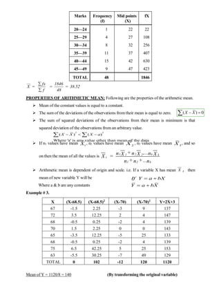
This document provides an introduction to statistics, including definitions, reasons for studying statistics, and the scope and importance of statistics. It discusses how statistics is used in fields like insurance, medicine, administration, banking, agriculture, business, and sciences. It also outlines the main functions of statistics and its branches, including theoretical, descriptive, inferential, and applied statistics. Finally, it covers topics related to data representation, including methods of presenting data through tables, graphs, and diagrams.

1. INTRODUCTORY STATISTICS
Definition of Statistics: - Statistics is defined as scientific technique used in collection,
presentation, analysis and interpretation of numerical data, and drawing inferences from these data.
Why Study Statistics?
No matter what line of work you select, you will find yourself faced with decisions where an
understanding of data analysis is helpful. In order to make an informed decision, you will need to be
able to:
 Determine whether the existing information is adequate or additional information is
required.
 Gather additional information, if it is needed, in such a way that it does not provide
misleading results.
 Summarize the information in a useful and informative manner.
 Analyze the available information.
 Draw conclusions and make inferences while assessing the risk of an incorrect conclusion.
Scope/ Importance of statistics
Statistics plays an important role in almost every field of humane life.
Insurance Companies:Insurance companies use statistical analysis to set rates for home,
automobile, life, and health insurance. Tables are available that summarize the probability that a 25-
year-old woman will survive the next year. Based on these probabilities, life insurance premiums
can be established.
Environment:The Environmental Protection Agency is interested in the water quality at a certain
city. They periodically take water samples to establish the level of contamination and maintain the
level of quality.
Medical Field:Medical researchers study the cure rates for diseases using different drugs and
different forms of treatment. For example, what is the effect of treating a certain type of knee injury
surgically or with physical therapy? If you take an aspirin each day, does that reduce your risk of a
heart attack?
Administration: Statistics plays an important role in the field of administration. A modern
administrator depends upon statistical data. Preparation of budget is impossible without statistical
record.
Banking:Statistical methods are helpful to the bankers. They can estimate the amount of money
that is required to fulfill the demands of depositors during various days of week.
Agriculture:Statistical methods help to study the comparison of various varieties of seed or
fertilizers.
Business& Economics:Statistical tools can be applied in the study of economic problems and the

2. business activity. A businessman depends upon statistical data for studying the need and desire of
consumer according to their tastes.
Moreover, statistics plays a vital role in all sciences like Physics, Chemistry, Biology,
Psychology, Sociology, Zoology and Botany.
Functions of statistics:
There are four main functions of statistics are
1. Collection of Data 2. Presentation of Data
3. Analysis of Data 4. Interpretation of Results
Branches of statistics:
Statistics can be divided in to following branches:
1. Theoretical Statistics 2. Descriptive Statistics
3. Inferential Statistics 4. Applied Statistics
Theoretical Statistics:It covers development of statistical distributions, experimental designs,
sampling designs, etc.
Descriptive Statistics:It is a branch of statistics that refers to the methods and principles of
collecting information and presenting such information in the form of tables and graphs.
Inferential Statistics:It is a branch of statistics that deals with procedures of drawing inferences
about the population on the basis of the sample information obtained from a sample.
Applied Statistics:It is a branch of statistics which is mainly covers, population, census, national
income, production, business statistics, industrial statistics, quality control, biostatistics, etc.
Population:A population is an aggregate of individuals, or objects or material about population
which some sort of information is required. OR The aggregate of objects with which we are
concerned is called population. e.g Heights of students in Statistics department is a population.
Number of observation in the population is denoted by “N” and is called population size.
Finite Population:A population is Finite if its individuals can be counted. For example, the
population of Universities in Vehari.
Infinite Population:A population is infinite if its individuals cannot be counted. For example,
population of stars in the sky.
Sample: Any representative part of population is known as sample. OR Any subset of a population
is called a sample. Number of observation in a sample is denoted by “n” and is called sample size.
e.g Heights of five students in statistics department selected from all students in statistics
department.
Parameter: Any numerical value describing a characteristic of a population is called a parameter. It
is usually denoted by Greek small letters. For example, population mean and Population standard
deviation .



3. Statistic:Any numerical value describing a characteristic of a sample is called a statistic. It is
usually denoted by Latin letters. For example, sample mean and sample standard deviation .
Constant: A quantity which can assume only one value is called constant. For example,
.
Observation: The numerically recording of information is called observation/datum.
Variable:A measurable quantity which changes from one individual to another individuals called
variable. For example, Speed of the car, Heights of students.
Types of Variable:
1. Quantitative variable 2. Qualitative variable/Attributes
Quantitative variable:The variables which can be numerically measured are called quantitative
variable. For example, Heights of students, Speed of car.
Types of Quantitative variable:
1. Discrete variable 2. Continuous variable
Discrete variable:A variable which can assume only some specific values or the values in whole
numbers with in a given range is called discrete variable. For example, No, of children in a family,
No, of chairs in a class room.
Continuous variable: A variable which can assume all possible values or the values in fraction
with in a given range is called continuous variable. For example, speed of car, heights of students.
Qualitative variable/Attributes: A variable which cannot be numerically measured, but only its
presence or absence can be described is called qualitative variable or attributes. For example, Sex,
Religion, Eyes colour, Beauty.
Data: The set of observations is called data.
Statistical Data: A sequence of observations, made on a set of objects included in the sample
drawn from a population is called statistical data. These observations may be obtained either by
counting or by measurement.
Ungrouped data/Raw data: Data which have not been condensed in the form of frequency
distribution are called ungrouped/Raw data.
Grouped data: The data which have been condensed in the form of frequency distribution are
called grouped data.
Primary data: Data obtained from the original or direct source and have not undergone any sort of
statistical treatment are called Primary data
Secondary data: Data that have undergone any sort of statistical treatment at least once are called
Secondary data.
Collection of primary data:
1. Direct personal investigation 2. Through Investigators 3. Through questionnaires. 4.
X S
7182
.
2

e 1415
.
3



4. Through local sources 5. Through telephone and Internet.
Collection of Secondary data:
1. Government organization 2. Semi- Government organizations 3. Newspapers
REPRESENTATION OF DATA
A major reason for calculating statistics is to describe and summarize a set of data. A mass of
numbers is not usually very informative so we need to find ways of abstracting the key information
that allows us to present the data in a clear and comprehensible form.
PRESENTATION OF DATA:
The raw data, which have been collected, are usually very large in quantity. Therefore, we have to
organize and summarize the collected data in such a form that is easy to understand.
Array: The arrangement of data in ascending or descending order of magnitude is called an array.
Different methods used in the presentation of statistical data
1. Classification 2. Tabulation 3. Diagram 4. Graph
Classification: Process of arranging the data into relatively homogenous groups or classes
according to some common characteristics is called classification. For example, population of the
country is classified according to age, sex, religion and marital status.
Tabulation: The systematic arrangement of the data in the form of rows and columns for the
purpose of comparison and analysis is known as tabulation.
Frequency distribution: A frequency distribution is a tabular arrangement of data in which various
items are arranged into classes or groups and the number of items falling in that class is stated. The
number of observations falling in a particular class is called class frequency and is denoted by "f".
Class and Class frequency: when a set of data are divided into non-overlapping homogeneous
groups, each group is called class or class interval. The number of observations falling in a
particular class is called frequency of that class or simply frequency and is denoted by "f".
Class limits: The class limits are defined as the number or the values of the variables which are
used to separate two classes. The smaller number is called lower class limit and larger number is
called upper class limit.
Class boundaries: The class boundaries are obtained by subtracting and adding half of the
difference between the upper limit and lower limit of two successive classes respectively. It can also
be obtained by subtracting and adding h/2 from midpoint of each class.
Class mark or mid points: The class mark or the midpoint is that value which divides a class into
two equal parts. It is obtained by dividing the sum of lower and upper class limits or class
boundaries of a class by 2.
Class interval: Class interval is the length of a class. A class interval is usually denoted by "h". It is
obtained by

5. (i) The difference between the upper-class boundary and the lower-class boundary.
(ii) The difference between either two successive lower or two successive upper class limits.
(iii) The difference between two successive midpoints.
CONSTRUCTION OF A FREQUENCY DISTRIBUTION:
Decide the number of classes: The number of classes is determining by the formula i.e.
K=1+3.3log(n) OR (approximately)
Where K denotes the number of classes and n denotes the total number of observations.
Determine the range of the data: The difference between the largest and smallest values in the
data is called the range of the data. i.e. R = largest observation - smallest observation
Where R denote the range of the data.
Determine the approximate size of class interval: The size of the class interval is determined by
dividing the range of the data by the number of classes i.e. h= R/K
Where h denotes the size of the class interval. In case of fractional results, the next higher whole
number is usually taken as the size of the class interval.
Decide where to locate the class limits: The lower-class limit of the first class is started just below
the smallest value in the data and then add class interval to get lower class limit of the next class,
repeat this process until the lower-class limit of the last class is achieved.
Distribute the data into appropriate classes:Take an observation and marked a vertical bar
"I"(Tally) against the class it belongs.
Cumulative Frequency:Cumulative frequency of a class is obtained by adding all the frequencies
of all preceding classes including that class and is denoted by c.f.
Relative Frequency: The frequency of a class divided by the total frequency of all the classes is
called Relative frequency and is denoted by r.f.
Cumulative relative frequency: Cumulative relative frequency of a class is obtained by adding all
the relative frequencies of all preceding classes including that class.
Percentage frequency: Percentage frequency of a class is obtained by multiplying100 to the
relative frequencies of that class.
Cumulative percentage frequency: Cumulative percentage frequency of a class is obtained by
adding all the percentage frequencies of all preceding classes including that class.
Example # 1. The following data is the final plant height (cm) of thirty plants of wheat. Construct a
frequency distribution
87 91 89 88 89 91 87 92 90 98 95 97 96 100
101 96 98 99 98 100 102 99 101 105 103 107 105 106
107 112
(i) Number of classes: The number of classes is determining by the formula
n
k 

6. K = 1+3.3 log(n) = 1+3.3 log (30)= 1+3.3(1.4771) = 5.87 ≈ 6
(ii) Size of class interval:The size of the class interval h= R/K
R = Largest observation - Smallest observation = 112 - 87 = 25
h = 25/6 = 4.17 ≈5
FREQUENCY DISTRIBUTION
Class
limits
Class
boundaries
Tally Frequency
f
Midpoint
X
c.f
Freq.
r.f
Freq.
%
frequency
Cumulative
% Freq.
86----90 85.5----90.5 6 88 6 0.2000 20.00 20.00
91----95 90.5----95.5 4 93 10 0.1333 13.33 33.33
96----100 95.5----100.5 10 98 20 0.3333 33.33 66.66
101----105 100.5----105.5 6 103 26 0.2000 20.00 86.66
106----110 105.5----110.5 3 108 29 0.1000 10.00 96.66
111----115 110.5----115.5 1 113 30 0.0333 3.33 99.99
30 1.0000 100
Example # 2. The following data represent the number of goals scored by a team in 10 matches
0,0,1,1,3,1,3,0,2,0 construct frequency distribution
Number of Goals
(X)
Number of Matches
(f)
0 4
1 3
2 1
3 2
Example # 3. The following data represent the gender of 10 students
Male, Male, Female, Male, Female, Male, Female, Male, Male, Female. Construct frequency
Distribution
Gender Number of Students
Male 6
Female 4
GRAPHICAL REPRESENTATION:The Visual representation of statistical data in the
form of points, lines, areas and other geometrical forms and symbols is known as graphical
representation. Such visual representation can be divided in to two groups.

7. (i) Graph (ii) Diagram
The basic difference between a graph and a diagram is that a graph is a representation of data by a
continuous curve, usually shown on graph paper while a diagram is any other one, two or three-
dimensional form of visual representation.
Diagrams: Diagram is a device used for representing a statistical data in such a way that it
provides maximum information’s about the movement of the data.
Advantages of Diagrams:
 The diagrams are good looking and attractive.
 The diagrams leave more effective and long lasting impression on the mind of a reader.
 The diagram make it easier to compare two or more things at a time.
Disadvantages of Diagrams:
 The diagrams are less accurate than tables.
 The diagrams have cost money and time and the amount of information conveyed is limited.
Types of Diagrams: Different types of diagram or charts commonly used for displaying statistical
data are described below:
1. Simple Bar Diagram/Chart 2. Multiple Bar Diagram/Chart
3. Sub-divided or Component Bar Diagram/Chart 4. Pie Diagram/Chart
Simple bar chart/Diagram: A Simple bar chart consists of horizontal or vertical bars of equal
widths and lengths proportional to the magnitudes of the observations. The space separating the bars
should not exceed the width of the bar and should not be less than half of its width. The data when
do not relate to time should be arranged in ascending or descending order before charting.
Multiple bar chart/Diagram: It is an extension of simple bar chart and is used to represent two or
more related sets of data in the form of groups of bars side by side. Multiple bar charts provide more
information’s about the same problem.
Sub-divided/component bar chart/Diagram: In Component bar chart, each bar is divided into
two or more sections. The length of the bar represents the total and various sections represent the
components of total. OR
Sub-divided bar chart is obtained by dividing simple bar chart in to different components.
Pie diagram/Diagram: A Pie diagram is the division of a circular region into different sectors of
any convenient radius. It is constructed by dividing the total. As a circle consists of 360o
is divided
into different components.
360
sec 

quantity
Whole
part
Component
tor
a
of
Angle
Graphs: Graph means the drawing of geometrical curves in conformity with the given data. It is a
representation of data by a continuous curve.

8. Advantages of Graphs:
 Graphs are most effective way to represent data.
 Graphs are the most effective way to compare two sets of data at a time.
 Graphs are helpful to show the general trend of data.
 Graphs are helpful in prediction and forecasting.
 Graphs are useful to locate some of the averages.
Types of graphs: Different types of graphs are commonly used for displaying statistical data:
(i) Historigram/Graph of time series (ii) Histogram
(iii) Frequency polygon & Frequency curve (iv) Cumulative Frequency polygon or Ogive
Historigram/Graph of time series: A graph of time series is called historigram. A Historigram is
constructed by taking time along X-axis and the value of the variable along Y-axis. Points are
plotted and are then connected by straight line segments to get the Historigram.
Histogram: Histogram is the graphical representation of frequency distribution by a set of adjacent
rectangles in which area of each rectangle is proportional to the corresponding frequency. In the
construction of histogram class boundaries taking along the X-axis and whose height are
proportional to the frequencies with respective classes (frequency along Y-axis).But in case of
unequal class interval adjusted frequency is used in place of frequency where adjusted frequency is
obtained by dividing the frequency to the class interval.
Frequency polygon: A frequency polygon is a line graph of frequency distribution in which the
frequencies are plotted against the mid points of the classes.It is constructed by taking the midpoints
along X-axis and class frequency along Y-axis. Points are plotted and are then connected by straight
line segments. But to get a polygon*
add extra class midpoint at both ends of the distribution with
zero frequency so that the polygon does form a closed figure with the horizontal axis.
Frequency curve: A frequency curve is constructed by taking the midpoints along X-axis and class
frequency along Y-axis. Points are plotted and are then connected by free hand curve.
Cumulative frequency polygon/Ogive: A Cumulative frequency polygon is obtained by plotting
the cumulated frequency (along Y-axis) against the upper-class boundaries (along X-axis) and the
points are joined by straight line segments. To get a polygon include lower class boundary of the
first class with zero frequency and joined the last point with the last upper class boundary.
Types of frequency curve:
(1) Symmetrical distribution (2) Skewed distribution
Symmetrical distribution: A frequency distribution or curve is said to be symmetrical if values
equidistant from a central maximum have the same frequencies. For example, Normal curve.
Skewed distribution A frequency distribution or curve is said to be skewed when it departs from
symmetry.

9. MEASURE OF CENTRAL TENDENCY
An average is a single value As an average tends to lie at the center of the distribution.
Average:
An average is a numerical value that is used to represent a set of data.
Properties of a good Average:A good average must have the following properties:
 It should be clearly defined by mathematical formula.
 It should be easy to calculate and simple to understand.
 It should be based on all observation of data.
 It should be capable for further algebraic treatment.
 It should be least affected by fluctuation of sampling.
 It should not be affected by extreme values.
Types of averages: The common used averages are:
(i) Arithmetic mean (ii) Geometric mean (iii) Harmonic mean
(iv) Median and quantiles (v) Mode
Arithmetic mean: Arithmetic mean (A.M) of a set of data is obtained by dividing the sum of all the
observations by the total number of observations. It is denoted by Greek letter "  ".read as “meu”
for the population data. Population mean for N values is given as
For ungrouped data
N
X
=
N
X
...
+
X
+
X
+
X
=
N
i
i
N


 1
3
2
1

The estimate of population mean  is the sample mean and is denoted by “ X ” read as “X-bar”
for the sample data. Sample mean for n values is given as
n
x
=
n
x
...
+
x
+
x
+
x
=
X
n
i
i
n


 1
3
2
1
Example # 1. Find the arithmetic mean for the following data set.
i
X = 87, 91, 89, 88, 89, 91, 87, 92, 90, 98.
2
.
90
10
902
=
=
n
x
=
X

When the number of observations is very large, the data is organized into a frequency distribution,
which is used to calculate the approximate values of descriptive measures as the identity of the
observations is lost.
For grouped data


 



n
i
i
n
i
i
i
n
i
i
n
n
f
x
f
=
f
x
f
...
+
x
f
+
x
f
+
x
f
=
X
1
1
1
3
3
2
2
1
1
Example # 2. Find the arithmetic mean for

10. Marks Frequency
(f)
Mid points
(X)
fX
20—24 1 22 22
25—29 4 27 108
30—34 8 32 256
35—39 11 37 407
40—44 15 42 630
45—49 9 47 423
TOTAL 48 1846
38.52
=
48
1846
=
f
fx
=
X


PROPERTIES OF ARITHMETIC MEAN: Following are the properties of the arithmetic mean.
 Mean of the constant values is equal to a constant.
 The sum of the deviations of the observations from their mean is equal to zero.
 The sum of squared deviations of the observations from their mean is minimum is that
squared deviation of the observations from an arbitrary value.
 If n1 values have mean 1
X , n2 values have mean 2
X , n3 values have mean 3
X , and so
on then the mean of all the values is 1 2 k
1 2 k
c
1 2 k
+ ,...
n n n
X X X
X =
+ +...
n n n
 Arithmetic mean is dependent of origin and scale. i.e. If a variable X has mean X , then
mean of new variable Y will be
Where a & b are any constants
Example # 3.
X (X-68.5) (X-68.5)2
(X-70) (X-70)2
Y=2X+3
67 -1.5 2.25 -3 9 137
72 3.5 12.25 2 4 147
68 -0.5 0.25 -2 4 139
70 1.5 2.25 0 0 143
65 -3.5 12.25 -5 25 133
68 -0.5 0.25 -2 4 139
75 6.5 42.25 5 25 153
63 -5.5 30.25 -7 49 129
TOTAL 0 102 -12 120 1120
Mean of Y = 1120/8 = 140 (By transforming the original variable)
( ) 0
X X
 

2 2
( ) ( )
Where 'a' is any value other than mean of the data
X X X a
  
 
If Y a bX
Y a bX
 
 

11. Mean of Y = 2 (68.5) + 3 = 140 (By using property)
Example # 4. The mean weight of 10 students is 50 Kg when two students left the class the
mean weight becomes 48 Kg find the mean weight of students who left the class
SOLUTION:-Total weight of 10 student = (10) (50) = 500
Total weight of 8 student (after 2 students left the class) = (8) (48) = 384
Total weight of 2 students ( Who left the class) = 500 - 384 = 116
Mean weight of the students who left the class = 116/2 = 58
Example # 5. For a class of 25 students, on Tuesday 20 students from the class took a Math test
and their mean marks was 80. On Friday remaining students from the class took the Math test
and their mean marks was 90. Find the mean marks of the entire class.
Total marks of 20 students who took test on Tuesday = (20) (80) = 1600
Total marks of 5 students who took test on Friday = (5) (90) = 450
Total marks of 25 students = 1600 + 450 = 2050
Mean marks of 25 students = 82
Example # 6. Ali Shah took five Math tests during the semester and the mean of his test score
was 85. If his mean after the first three was 83, What was the mean of his 4th and 5th tests
SOLUTION:-
Total marks of all five tests = (5) (85) = 425
Total marks of first three tests = (3) (83) = 249
Total marks of last two tests = 425 – 249 = 176
Mean marks of last two tests = 88
Example # 7. If mean marks of students from three sections A, B and C are 45, 40 and 35
respectively with number of students from three section are 50, 40 and 60. Find mean marks of
students from three section ( Combined mean)
Solution:- Total marks of 50 students from Section A= (50) (45) = 2250
Total marks of 40 students from Section B = (40) (40) = 1600
Total marks of 60 students from Section C= (60) (35) = 2100
Total marks of 150 students from three sections = 5950
Mean marks of 150 students from three sections = 39.67
Merits of Arithmetic Mean:
 It is clearly defined by mathematical formula.
 It is easy to calculate and simple to understand.
 It is based on all the observations.
 It is capable for further algebraic treatments.
 It is least affected by sampling fluctuation.

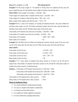
12. De-Merits of Arithmetic Mean:
 It is not an appropriate average for highly-skewed distribution.
 It is greatly affected by by extreme values.
 It cannot be calculated for open-end classes.
 It may be a value which is usually not present in the data.
 It cannot be computed accurately even one item is missing.
 Aleast one value will be greater and atleast one will be less than mean.
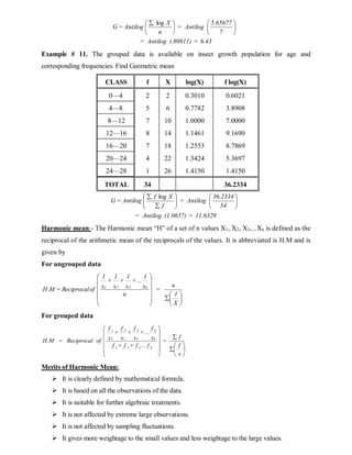
 Geometric mean and Harmonic mean are useful measure of central tendency for averaging
rates and ratios.
Geometric mean:- The geometric mean is the nth
root of the product of n positive values.
For ungrouped data )
X
X
X
(X
=
G n
1
n
*
...
*
*
* 3
2
1 OR





 

n
X
Antilog
=
G
n
X
=
n
]
X
...
x
+
x
[
=
G k
2
1
log
log
log
log
log
Log
For grouped data  f
f
n
f
f
f n
X
X
X
X
=
G
1
3
2
1 )
(
*
...
*
)
(
*
)
(
*
)
( 3
2
1
Where, n denote total number of classes OR












f
X
f
Antilog
=
G
f
X
f
=
f
...
f
+
f
+
f
X
f
...
X
f
+
X
f
+
X
f
=
G
n
3
2
1
n
n
3
3
2
2
1
1
log
log
log
log
log
log
Log
Merits of Geometric Mean:
 It is clearly defined by mathematical formula.
 It is based on all the observations.
 It is least affected by extreme values.
 It is suitable for further algebraic treatments.
 It gives equal weights to all the values.
 It is an appropriate average for averaging rates of change and ratios.
De-Merits of Geometric Mean:
 It is neither easy to calculate nor simple to understand.
 It cannot be calculated if any value is zero or negative in the data.
 It cannot be calculated in case of open-end frequency distribution.
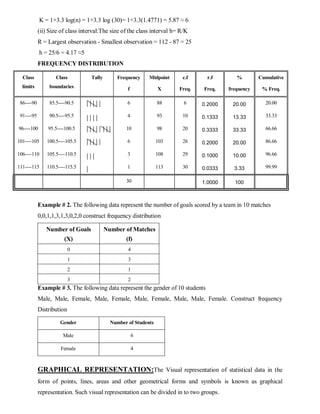
Example # 10. Find the Geometric mean of the values 3, 5, 6, 6, 7, 10, 12.
X 3 5 6 6 7 10 12 Total
log(X) .4771 .6989 .7782 .7782 .8451 1.000 1.0792 5.65677

13. 6.43
=
(.80811)
Antilog
=
7
5.65677
Antilog
=
n
X
Antilog
=
G 










  log
Example # 11. The grouped data is available on insect growth population for age and
corresponding frequencies. Find Geometric mean
11.6329
=
(1.0657)
Antilog
=
34
36.2334
Antilog
=
f
X
f
Antilog
=
G 














 log
Harmonic mean:- The Harmonic mean “H” of a set of n values X1, X2, X3,...Xn is defined as the
reciprocal of the arithmetic mean of the reciprocals of the values. It is abbreviated is H.M and is
given by
For ungrouped data



















X
1
n
=
n
x
1
...
+
x
1
+
x
1
+
x
1
of
Reciprocal
=
M
H k
3
2
1
.
For grouped data




















x
f
f
=
f
...
f
+
f
+
f
x
f
...
+
x
f
+
x
f
+
x
f
of
Reciprocal
=
M
H
k
3
2
1
k
k
3
3
2
2
1
1
.
Merits of Harmonic Mean:
 It is clearly defined by mathematical formula.
 It is based on all the observations of the data.
 It is suitable for further algebraic treatments.
 It is not affected by extreme large observations.
 It is not affected by sampling fluctuations.
 It gives more weightage to the small values and less weightage to the large values.
CLASS f X log(X) f log(X)
0—4 2 2 0.3010 0.6021
4—8 5 6 0.7782 3.8908
8—12 7 10 1.0000 7.0000
12—16 8 14 1.1461 9.1690
16—20 7 18 1.2553 8.7869
20—24 4 22 1.3424 5.3697
24—28 1 26 1.4150 1.4150
TOTAL 34 36.2334

14.  It is better than weighted mean since in this, values are automatically weighted.
De-Merits of Harmonic Mean:
 It is neither easy to calculate nor simple to understand.
 It cannot be calculated if any value of the data is zero.
 It is affected by extremely small observations.
 It may be a value which is usually not present in the data.
Example # 12. Calculate Harmonic mean for the following data
CLASS f X 1/X f (1/X)
0--4 2 2 0.5000 1.0000
4--8 5 6 0.1667 0.8333
8--12 7 10 0.1000 0.7000
12--16 8 14 0.7114 0.5714
16--20 7 18 0.0556 0.3889
20--24 4 22 0.0385 0.1818
24--28 1 26 1.4150 0.0385
TOTAL 34 3.7139
9.15
=
3.7139
34
=
x
f
f
=
H


Relation between A.M, G.M &H.M M
H
M
G
M
A .
.
. 
 M
A
M
G
M
H .
.
. 

The three means are equal only when all the observations are identical. A.M = G.M = H.M
M
H
M
A
M
G .
*
.
. 
Example # 13. Verify the relation A.M > G.M > H.M for the following
CLASS f X fX logX f logX 1/X f/X
1---3 5 2 10 0.30103 1.5051 0.500 2.500
4---6 8 5 40 0.69897 5.5918 0.200 1.600
7---9 12 8 96 0.90309 10.8371 0.125 1.500
10---12 9 11 99 1.04139 9.3725 0.091 0.818
13---15 3 14 42 1.14613 3.4384 0.071 0.214
TOTAL 37 287 30.7449 6.632
A.M = 7.76 > G.M = 6.78 > H.M = 5.57
Median & Quantiles:-
Median: Median is defined as the middle value of the data when the data is arranged in
ascending or descending order of magnitude. The median is a value that divides a set of data in

15. to two equal parts after arranging the values in ascending order of magnitude. It is simply the
middle value of the data when the number of values is odd. It is the mean of two middle values if
the number of values is even. Median is denoted by “ X
~
” read as X-childa or Tilda.
In both cases
For ungrouped data Median=Size of
th
n





 
2
1
item.
Merits of Median:
 It is easy to calculate and simple to understand.
 It is not affected by extreme values.
 It can be calculated for open-end frequency distribution.
 It is a useful average, when data are of qualitative nature.
 It is appropriate average for highly skewed distribution.
De-Merits of Median:
 It is not clearly defined by mathematical formula.
 It is not based on all the values.
 It is not suitable for further algebraic treatments.
 It is affected by sampling fluctuations.
 It is difficult to arrange a large number of values.
Example # 14. Given below are the marks obtained by 20 students.
53, 74, 82, 42, 39, 28, 20, 81, 68, 58, 54, 93, 70, 30, 61, 55, 36, 37, 29, 94. Find Median
Solution:-First arrange the data in ascending order of magnitude
20, 28, 29, 30, 36, 37, 39, 42, 53, 54, 55, 58, 61, 68, 70, 74, 81, 82, 93, 94.
Median = Size of
th
n





 
2
1
item = 10.5th
item
= Size of 10.5th
item = 10th
+ 0.5(11th
- 10th
)
Median = 54 + 0.5(55 - 54) = 54.5
50% i.e. 10 students obtained marks 54.5 or below
Quantiles: Quantiles are the values that divides a set of data in to more than two equal parts.
Quartiles, Deciles and Percentiles are collectively called Quantiles.
often, we are interested to know the position of an observation in the set of data. We are
interested to know the percentage of students having height less than some specific value. The
measure used for this purpose are called quantiles or fractiles and are usually calculated under
the following headings.
I) Quartiles II) Deciles III) Percentiles
Quartiles: Quartiles are the values that divide a set of data in to four equal parts after arranging
them in ascending or descending order of magnitude. Quartiles are denoted by Q1, Q2,and Q3.

16. Q1is called lower-quartile, Q3 is called upper-quartile and Q2 is also called median
For ungroup data
3
,
2
,
1
4
1






 
j
where
n
observatio
n
j
of
Size
=
Q
th
j
item
item
n
of
Size
Q th
th
25
.
5
4
1
1
1 





 

Size of 5 .25th
item =5th
+0.25(6th
-5th
)
=36+0.25(37-36)=36.25
Q1 = 36.25, indicates that 25% students (i.e. 5) have marks 36.25 or below OR 75% students
(i.e. 15) have marks 36.25 or above.
item
item
n
of
Size
Q th
th
75
.
15
4
1
3
3 





 

Size of 15.75th
item =15th
+0.75(16th
-15th
)
=70+0.75(74-70)=73
Q3 = 73, indicates that75% students (i.e. 15) have marks 73 or below OR 25% students (i.e. 25)
have marks 73 or above
Deciles:- Deciles are the values that divide a set of data in to ten equal parts after arranging them
in ascending order of magnitude. Deciles are denoted by D1, D2, D3...D9.
For ungrouped data
9
3
,
2
,
1
10
1







 
j
where
n
observatio
n
j
of
Size
=
D
th
j
Percentiles:-Percentiles are the values that divide a set of data in to 100 equal parts after
arranging them in ascending order of magnitude. Percentiles are denoted by P1, P2, P3...P99.
For ungrouped data
99
3
,
2
,
1
100
1







 
j
where
n
observatio
n
j
of
Size
=
P
th
j
Median and Quantiles for group data






c
-
2
n
f
h
+
l
=
Median
l=Lower class boundary of the class containing median
h=class interval of the class containing median*
f=Frequency of the class containing median
n=Total number of observations
C=Cumulative frequency of the class preceding the class containing median.
*The median class is a class which corresponds to the cumulative frequency in which (n/2) lies.

17. Example # 15. Estimate the Median and the Quartiles
Daily Income (Rs. 00) f cf Class Boundaries
5-----24 4 4 4.5---24.5
25-----44 6 10 24.5---44.5
45-----64 14 24 44.5---64.5
65-----84 22 46 64.5---84.5
85----104 14 60 84.5---104.5
105---124 5 65 104.5---124.5
125---144 7 72 124.5---144.5
145---164 3 75 144.5---164.5
Since n/2 = 75/2 = 37.5
So the class containing median is 64.5------84.5
76.77
=
24
-
2
75
22
20
+
64.5
c
-
2
n
f
h
+
l
=
Median 












Quartiles for group data












C
-
4
n
j
f
h
+
l
=
Qj
l= Lower class boundary of the class containing jth
quartile
(i.e the class corresponding to the cumulative frequency in which 'j(n/4)th
' observation lies).
h= Class interval of the class containing jth
quartile
f= Frequency of the class containing jth
quartile
n= Total number of observations
C= Cumulative frequency of the class preceding the class containing jth
quartile.
Calculate Q1, Q3, D3 & P70
Since n/4 = 75/4 = 18.75
So the class containing Q1 is 44.5-----64.5
57
10
75
1
14
20
5
.
44
1 












-
4
+
=
Q
Since 3n/4 = 225/4 = 56.25
So the class containing Q3 is 64.5-----84.5
Since 3n/10 = 225/10 = 22.5
So the class containing D3 is 44.5-----64.5
14
.
99
46
75
3
14
20
5
.
84
3 












-
4
+
=
Q

18. 35
.
62
10
10
75
3
14
20
5
.
44
3 












-
+
=
D
Since 7n/100 = 525/100 = 5.25
So the class containing P70 is 24.5-----44.5
66
.
28
4
100
75
7
6
20
5
.
24
3 












-
+
=
P
Mode:- The mode is defined as that value in the data which occurs the greatest number of time
provided such a value exists. A set of data may have more than one mode or no mode at all when
each observation occurs the same number of time. A distribution having only one mode is called
Uni-modal distribution, having two modes is called bi-modal distribution and a distribution
having more than two modes is called a multi-model distribution.
For grouped data
Where
l= Lower class boundary of the class containing mode (i.e the class corresponding to the highest
frequency)
h= class interval of the class containing mode
fm=Frequency of the class containing mode
f1=Frequency of the class preceding the class containing mode
f2=Frequency of the class following the class containing mode
Merits of Mode:
 It is easy to calculate and simple to understand.
 It is not affected by extreme values.
 It is suitable average for qualitative data.
 It can be located even in open end classes.
De-Merits of Mode:
 It is an ill-defined average..
 It is not based on all the values.
 It is not suitable for further algebraic treatments.
 It is affected by sampling fluctuations.
xh
)
f
-
f
(
+
)
f
-
f
(
f
-
f
+
l
=
Mode
2
m
1
m
1
m

19. Example # 16. Calculate Mode for the data
Weight No of students Class boundaries
118----126 3 117.5----126.5
127----135 5 126.5----135.5
136----144 9 135.5----144.5
145----153 12 144.5----153.5
154----162 5 153.5----162.5
163----171 4 162.5----171.5
172----180 2 171.5----180.5
Since heights frequency is 12
So the class containing Mode is 144.5----153.5
147.2
=
x9
5)
-
(12
+
9)
-
(12
9
-
12
+
144.5
=
Mode
xh
)
f
-
f
(
+
)
f
-
f
(
f
-
f
+
l
=
Mode
2
m
1
m
1
m
NOTE:- (i) A data may have more than one mode or no-mode atall
(ii) A data with one mode is called uni-model, 2 modes bi-model or more than 2 modes multi model
data
Relation between mean, median, mode.
Mean = Median = Mode For symmetrical distribution
Mean > Median > Mode For positively skewed distribution
Mean < Median < Mode For negatively skewed distribution
For skewed distribution
Mode = 3 Median – 2 Mean