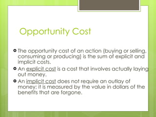
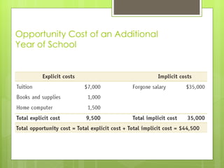
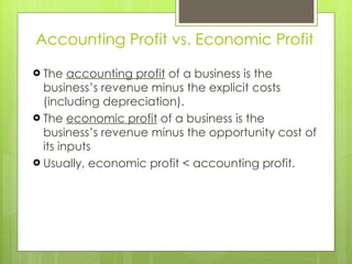
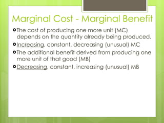
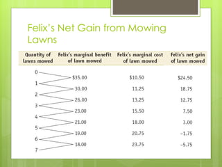
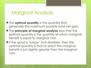
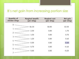
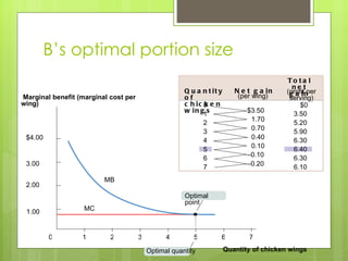
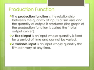
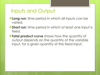
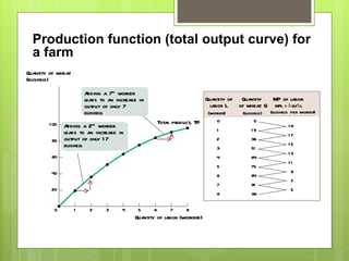
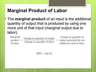
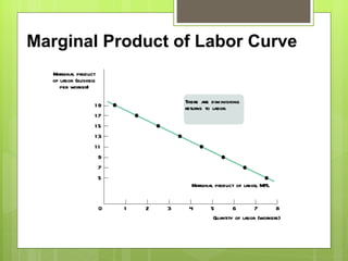
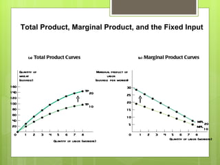
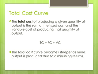
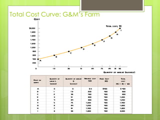
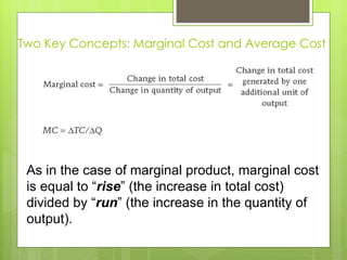
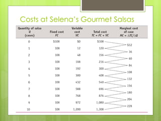
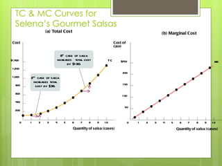
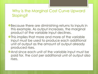
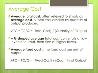
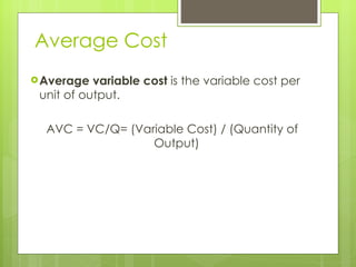
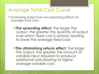
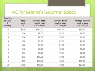
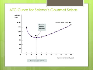
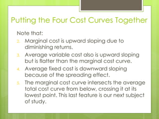
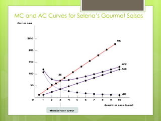
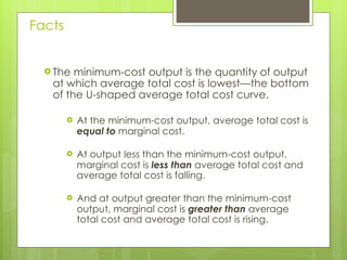
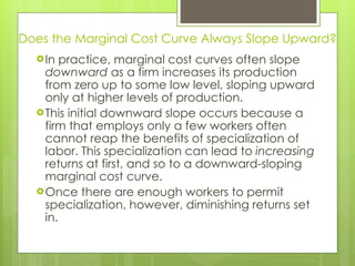
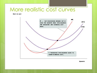
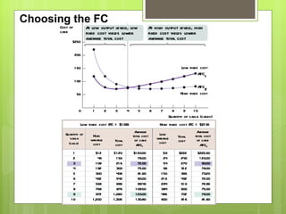
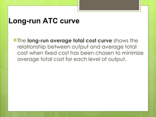
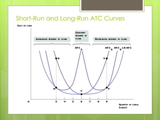
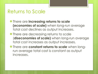
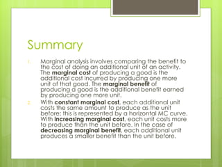
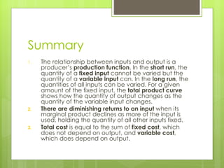
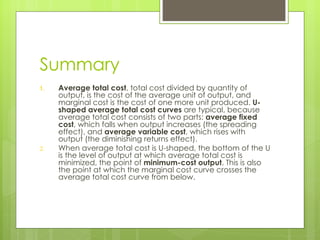
The document provides an overview of key concepts related to marginal analysis, inputs, outputs, and costs. It discusses marginal and average quantities, production functions, fixed and variable inputs, diminishing returns, fixed and variable costs, total cost, marginal and average cost, short-term and long-term costs, and returns to scale. Key terms like marginal cost, marginal benefit, total cost curves, average cost curves, and their relationships are defined.
Income elasticity of demand is the degree of responsiveness of quantity demanded of a commodity due to change in consumerโs income, other things remaining constant. In other words, it measures by how much the quantity demanded changes with respect ot the change in income.
FellowBuddy.com is an innovative platform that brings students together to share notes, exam papers, study guides, project reports and presentation for upcoming exams.
We connect Students who have an understanding of course material with Students who need help.
Benefits:-
# Students can catch up on notes they missed because of an absence.
# Underachievers can find peer developed notes that break down lecture and study material in a way that they can understand
# Students can earn better grades, save time and study effectively
Our Vision & Mission โ Simplifying Students Life
Our Belief โ โThe great breakthrough in your life comes when you realize it, that you can learn anything you need to learn; to accomplish any goal that you have set for yourself. This means there are no limits on what you can be, have or do.โ
Like Us - https://www.facebook.com/FellowBuddycom
๏ข Isoquant is also called as equal product curve or production indifference curve or constant product curve. Isoquant indicates various combinations of two factors of production which give the same level of output per unit of time.
๏ข Just as an indifference curve represents various combinations of two goods which give a consumer equal amount of satisfaction, an iso-product curve shows all possible combinations of two inputs physically capable of producing a given level of output. Since an iso-product curve represents those combinations which will result in the production of an equal quantity of output, the producer would be indifferent between them.
๏ข This law was given by Alfred Marshall in his book principle of economics.
๏ข It show particular pattern of change in output when some factor remain fixed.
๏ข Production depend upon factors of production , if factors of production are good, production may increase and vice-versa.
๏ข Production function show functional relationship between production and factors of production.
๏ข It refers to manner of change in output cost by the increase in all the input simultaneously and in the same proportion.
๏ข Returns refers to โchange in physical outputโ
๏ข Scale refers to โquantity of input employedโ
๏ข Change in scale means that all factors of production are increased or decreased in same proportion.
๏ข The cost advantage that arises with increased output of a product.
๏ข It arises because of the inverse relationship between the quantity produced and per-unit fixed cost.
๏ข Profit refers to the excess of receipts from the sale of goods over the expenditure incurred on producing them.
๏ข The amount received from the sale of goods is known as โrevenueโ and the expenditure on production of such goods is termed as โcostโ. The difference between revenue and cost is known as โprofitโ.
๏ข For example, if a firm sells goods for Rs. 10 crores after incurring an expenditure of Rs. 7 crores, then profit will be Rs. 3 crores.
Cost Functions
Cost Concepts Defined
Short-Run Cost Curves
Long-Run: Optimal Combination of Inputs
Constrained Cost Minimization: Lagrangian Multiplier Method
The U Shape of the LAC Curve
The firm is an economic institution that transforms factors of production into consumer goods โ it:
Organizes factors of production.
Produces goods and services.
Sells produced goods and services.
The Cost Of Production - Dealing with Cost - Explicit and Implicit Cost - Eco...FaHaD .H. NooR
ย
Economics #UCP
What is 'Production Cost'
Production cost refers to the cost incurred by a business when manufacturing a good or providing a service. Production costs include a variety of expenses including, but not limited to, labor, raw materials, consumable manufacturing supplies and general overhead. Additionally, any taxes levied by the government or royalties owed by natural resource extracting companies are also considered production costs.
BREAKING DOWN 'Production Cost'
Also referred to as the cost of production, production costs include expenditures relating to the manufacturing or creation of goods or services. For a cost to qualify as a production cost it must be directly tied to the generation of revenue for the company. Manufacturers experience product costs relating to both the materials required to create an item as well as the labor need to create it. Service industries experience production costs in regards to the labor required to provide the service as well as any materials costs involved in providing the aforementioned service.
In production, there are direct costs and indirect costs. For example, direct costs for manufacturing an automobile are materials such as the plastic and metal materials used as well as the labor required to produce the finished product. Indirect costs include overhead such as rent, administrative salaries or utility expenses.
Deriving Unit Costs for Product Pricing
To figure out the cost of production per unit, the cost of production is divided by the number of units produced. Once the cost per unit is determined, the information can be used to help develop an appropriate sales price for the completed item. In order to break even, the sales price must cover the cost per unit. Amounts above the cost per unit are often seen as profit while amounts below the cost per unit result in losses.
Micro review 1 for International Economics' students: the simple market model.
If you download this on a computer at the college (or open it on a computer that has PowerPoint), you'll be able to read detailed notes for each slide.
Discussion of elasticity (price-elasticity of demand and supply, income elasticity of demand, and cross-price elasticity of demand) for my Principles of Microeconomics students.
Putting the SPARK into Virtual Training.pptxCynthia Clay
ย
This 60-minute webinar, sponsored by Adobe, was delivered for the Training Mag Network. It explored the five elements of SPARK: Storytelling, Purpose, Action, Relationships, and Kudos. Knowing how to tell a well-structured story is key to building long-term memory. Stating a clear purpose that doesn't take away from the discovery learning process is critical. Ensuring that people move from theory to practical application is imperative. Creating strong social learning is the key to commitment and engagement. Validating and affirming participants' comments is the way to create a positive learning environment.
LA HUG - Video Testimonials with Chynna Morgan - June 2024Lital Barkan
ย
Have you ever heard that user-generated content or video testimonials can take your brand to the next level? We will explore how you can effectively use video testimonials to leverage and boost your sales, content strategy, and increase your CRM data.๐คฏ
We will dig deeper into:
1. How to capture video testimonials that convert from your audience ๐ฅ
2. How to leverage your testimonials to boost your sales ๐ฒ
3. How you can capture more CRM data to understand your audience better through video testimonials. ๐
"๐ฉ๐ฌ๐ฎ๐ผ๐ต ๐พ๐ฐ๐ป๐ฏ ๐ป๐ฑ ๐ฐ๐บ ๐ฏ๐จ๐ณ๐ญ ๐ซ๐ถ๐ต๐ฌ"
๐๐ ๐๐จ๐ฆ๐ฌ (๐๐ ๐๐จ๐ฆ๐ฆ๐ฎ๐ง๐ข๐๐๐ญ๐ข๐จ๐ง๐ฌ) is a professional event agency that includes experts in the event-organizing market in Vietnam, Korea, and ASEAN countries. We provide unlimited types of events from Music concerts, Fan meetings, and Culture festivals to Corporate events, Internal company events, Golf tournaments, MICE events, and Exhibitions.
๐๐ ๐๐จ๐ฆ๐ฌ provides unlimited package services including such as Event organizing, Event planning, Event production, Manpower, PR marketing, Design 2D/3D, VIP protocols, Interpreter agency, etc.
Sports events - Golf competitions/billiards competitions/company sports events: dynamic and challenging
โญ ๐ ๐๐๐ญ๐ฎ๐ซ๐๐ ๐ฉ๐ซ๐จ๐ฃ๐๐๐ญ๐ฌ:
โข 2024 BAEKHYUN [Lonsdaleite] IN HO CHI MINH
โข SUPER JUNIOR-L.S.S. THE SHOW : Th3ee Guys in HO CHI MINH
โขFreenBecky 1st Fan Meeting in Vietnam
โขCHILDREN ART EXHIBITION 2024: BEYOND BARRIERS
โข WOW K-Music Festival 2023
โข Winner [CROSS] Tour in HCM
โข Super Show 9 in HCM with Super Junior
โข HCMC - Gyeongsangbuk-do Culture and Tourism Festival
โข Korean Vietnam Partnership - Fair with LG
โข Korean President visits Samsung Electronics R&D Center
โข Vietnam Food Expo with Lotte Wellfood
"๐๐ฏ๐๐ซ๐ฒ ๐๐ฏ๐๐ง๐ญ ๐ข๐ฌ ๐ ๐ฌ๐ญ๐จ๐ซ๐ฒ, ๐ ๐ฌ๐ฉ๐๐๐ข๐๐ฅ ๐ฃ๐จ๐ฎ๐ซ๐ง๐๐ฒ. ๐๐ ๐๐ฅ๐ฐ๐๐ฒ๐ฌ ๐๐๐ฅ๐ข๐๐ฏ๐ ๐ญ๐ก๐๐ญ ๐ฌ๐ก๐จ๐ซ๐ญ๐ฅ๐ฒ ๐ฒ๐จ๐ฎ ๐ฐ๐ข๐ฅ๐ฅ ๐๐ ๐ ๐ฉ๐๐ซ๐ญ ๐จ๐ ๐จ๐ฎ๐ซ ๐ฌ๐ญ๐จ๐ซ๐ข๐๐ฌ."
The world of search engine optimization (SEO) is buzzing with discussions after Google confirmed that around 2,500 leaked internal documents related to its Search feature are indeed authentic. The revelation has sparked significant concerns within the SEO community. The leaked documents were initially reported by SEO experts Rand Fishkin and Mike King, igniting widespread analysis and discourse. For More Info:- https://news.arihantwebtech.com/search-disrupted-googles-leaked-documents-rock-the-seo-world/
Personal Brand Statement:
As an Army veteran dedicated to lifelong learning, I bring a disciplined, strategic mindset to my pursuits. I am constantly expanding my knowledge to innovate and lead effectively. My journey is driven by a commitment to excellence, and to make a meaningful impact in the world.
Discover the innovative and creative projects that highlight my journey throu...dylandmeas
ย
Discover the innovative and creative projects that highlight my journey throughย Full Sail University. Below, youโll find a collection of my work showcasing my skills and expertise in digital marketing, event planning, and media production.
What are the main advantages of using HR recruiter services.pdfHumanResourceDimensi1
ย
HR recruiter services offer top talents to companies according to their specific needs. They handle all recruitment tasks from job posting to onboarding and help companies concentrate on their business growth. With their expertise and years of experience, they streamline the hiring process and save time and resources for the company.
Business Valuation Principles for EntrepreneursBen Wann
ย
This insightful presentation is designed to equip entrepreneurs with the essential knowledge and tools needed to accurately value their businesses. Understanding business valuation is crucial for making informed decisions, whether you're seeking investment, planning to sell, or simply want to gauge your company's worth.
What is the TDS Return Filing Due Date for FY 2024-25.pdfseoforlegalpillers
ย
It is crucial for the taxpayers to understand about the TDS Return Filing Due Date, so that they can fulfill your TDS obligations efficiently. Taxpayers can avoid penalties by sticking to the deadlines and by accurate filing of TDS. Timely filing of TDS will make sure about the availability of tax credits. You can also seek the professional guidance of experts like Legal Pillers for timely filing of the TDS Return.
3.0 Project 2_ Developing My Brand Identity Kit.pptxtanyjahb
ย
A personal brand exploration presentation summarizes an individual's unique qualities and goals, covering strengths, values, passions, and target audience. It helps individuals understand what makes them stand out, their desired image, and how they aim to achieve it.
18. B โs optimal portion size 7 6 5 4 3 2 1 0 $4.00 3.00 2.00 1.00 Marginal benefit (marginal cost per wing) Quantity of chicken wings Optimal point MC MB Optimal quantity 0 1 2 3 4 5 6 7 Total net gain (profit per serving) Net gain (per wing) Quantity of chicken wings $0 3.50 5.20 5.90 6.30 6.40 6.30 6.10 $3.50 1.70 0.70 0.40 0.10 โ 0.10 โ 0.20
19.
20.
21.
22. Production function (total output curve) for a farm 0 1 2 3 4 5 6 7 8 19 17 15 13 11 9 7 5 0 19 36 51 64 75 84 91 96 Quantity of labor L (worker) Quantity of wheat Q (bushels) MP of labor MPL = ๏ Q / ๏ L (bushels per worker) 7 8 6 5 4 3 2 1 0 100 80 60 40 20 Quantity of wheat (bushels) Quantity of labor (workers) Total product, TP Adding a 7 th worker leads to an increase in output of only 7 bushels Adding a 2 nd worker leads to an increase in output of only 17 bushels
23.
24.
25. Marginal Product of Labor Curve Marginal product of labor, MPL 7 8 6 5 4 3 2 1 0 19 17 15 13 11 9 7 5 Marginal product of labor (bushels per worker) Quantity of labor (workers) There are diminishing returns to labor.
26. (a) Total Product Curves (b) Marginal Product Curves Marginal product of labor (bushels per worker) Quantity of wheat (bushels) 7 8 6 5 4 3 2 1 0 30 25 20 15 10 5 7 8 6 5 4 3 2 1 0 160 140 120 100 80 60 40 20 TP 20 TP 10 MPL 20 MPL 10 Quantity of labor (workers) Quantity of labor (workers) Total Product, Marginal Product, and the Fixed Input
27.
28.
29. Total Cost Curve: G&M โs Farm 19 36 51 64 75 84 91 96 0 $2,000 1,800 1,600 1,400 1,200 1,000 800 600 400 200 Cost Quantity of wheat (bushels) A B C D E F G Total cost, TC H I A B C D E F G H I Point on graph 0 1 2 3 4 5 6 7 8 $400 400 400 400 400 400 400 400 400 O 200 400 600 800 1,000 1,200 1,400 1,600 400 600 800 1,000 1,200 1,400 1,600 1,800 2,000 0 19 36 51 64 75 84 91 96 Variable cost (VC) Total cost (TC = FC + VC) $ $ Quantity of labor L (worker) Quantity of wheat Q (bushels) Fixed Cost (FC)
30. Two Key Concepts: Marginal Cost and Average Cost As in the case of marginal product, marginal cost is equal to โ rise โ (the increase in total cost) divided by โ run โ (the increase in the quantity of output).
32. TC & MC Curves for Selena โs Gourmet Salsas $250 200 150 100 50 Cost of case 7 8 9 10 6 5 4 3 2 1 0 $1,400 1,200 1,000 800 600 400 200 Cost Quantity of salsa (cases) 7 8 9 10 6 5 4 3 2 1 0 (b) Marginal Cost (a) Total Cost T C MC Quantity of salsa (cases) 8 th case of salsa increases total cost by $180. 2 nd case of salsa increases total cost by $36.
38. ATC Curve for Selena โs Gourmet Salsas Average total cost, ATC M 7 8 9 10 6 5 4 3 2 1 0 $140 120 100 80 60 40 20 Minimum average total cost Minimum-cost output Cost of case Quantity of salsa (cases)
39.
40. MC and AC Curves for Selena โs Gourmet Salsas $250 200 150 100 50 7 8 9 10 6 5 4 3 2 1 M 0 MC A T C A VC AFC Minimum-cost output Cost of case Quantity of salsa (cases)
41.
42. Relationship between ATC and the MC Curves Cost of unit Quantity MC A T C MC L MC H A 1 B 1 A 2 B 2 M If marginal cost is above average total cost, average total cost is rising. If marginal cost is below average total cost, average total cost is falling.
43.
44. More realistic cost curves MC A T C A VC Cost of unit Quantity 2. โฆ but diminishing returns set in once the benefits from specialization are exhausted and marginal cost rises. 1. Increasing specialization leads to lower marginal costโฆ
45.
46. Choosing the FC $250 200 150 100 50 Cost of case Quantity of salsa (cases) 7 8 9 10 6 5 4 3 2 1 0 High fixed cost Low fixed cost A T C 2 A T C 1 At low output levels, low fixed cost yields lower average total cost At high output levels, high fixed cost yields lower average total cost A T C 1 12 48 108 192 300 432 588 768 972 1,200 $ 120 156 216 300 408 540 696 876 1,080 1,308 Total cost $ A T C 2 6 24 54 96 150 216 294 384 486 600 $ $222 240 270 312 366 432 510 600 702 816 Low fixed cost (FC = $108) High fixed cost (FC = $216) $120.00 78.00 72.00 75.00 81.60 90.00 99.43 109.50 120.00 130.80 $222.00 120.00 90.00 78.00 73.20 72.00 72.86 75.00 78.00 81.60 1 2 3 4 5 6 7 8 9 10 Average total cost of case Quantity of salsa (salsa) High variable cost Low variable cost Total cost Average total cost of case
47.
48. Short-Run and Long-Run ATC Curves B A T C 6 A T C 9 A T C 3 L R A T C 3 5 8 4 7 0 6 9 Increasing returns to scale Decreasing returns to scale Constant returns to scale C X A Y Cost of case Quantity of salsa (cases)
49.
50.
51.
52.
53.
54.
55.
Editor's Notes
Figure Caption: Figure 9-1: Marginal Cost The height of each shaded bar corresponds to Babette โs marginal cost of producing an additional chicken wing per serving. The height of each bar here is the same, $0.80, because Babette has constant marginal cost. So Babetteโs marginal cost curve, the line connecting the midpoints at the top of each bar, is horizontal.
Figure Caption: Figure 9-2: Marginal Benefit The height of each shaded bar corresponds to Babette โs marginal benefit of producing an additional chicken wing per serving. The height of each bar is lower than the one preceding it because Babette has decreasing marginal benefit. That is, the additional amount that Babetteโs customers are willing to pay for an additional chicken wing falls as the portion size gets larger and larger. As a result, Babetteโs marginal benefit curve, the curve connecting the midpoints at the top of each bar, slopes downward.
Figure Caption: Figure 9-3: Babette โs Optimal Portion Size The optimal quantity is the quantity that generates the highest possible total net gain. It is the quantity at which marginal benefit is equal to marginal cost. Equivalently, it is the quantity at which marginal benefit and marginal cost curves intersect. Here, they intersect at a portion size of approximately 5 wings. The table confirms that 5 is indeed the optimal quantity: it leads to the maximum total net gain, or profit, of $6.40.
Figure Caption: Figure 12-1: Production Function and Total Product Curve for George and Martha โs Farm The table shows the production function, the relationship between the quantity of the variable input (labor, measured in number of workers) and the quantity of output (wheat, measured in bushels) for a given quantity of the fixed input. It also calculates the marginal product of labor on George and Martha โs farm. The total product curve shows the production function graphically. It slopes upward because more wheat is produced as more workers are employed. It also becomes flatter because the marginal product of labor declines as more and more workers are employed.
Figure Caption: Figure 12-2: Marginal Product of Labor Curve for George and Martha โs Farm The marginal product of labor curve plots each worker โs marginal product, the increase in the quantity of output generated by each additional worker. The change in the quantity of output is measured on the vertical axis and the number of workers employed on the horizontal axis. The first worker employed generates an increase in output of 19 bushels, the second worker generates an increase of 17 bushels, and so on. The curve slopes downward due to diminishing returns to labor.
Figure Caption: Figure 12-3: Total Product, Marginal Product, and the Fixed Input This figure shows how the quantity of outputโillustrated by the total product curveโand marginal product depend on the level of the fixed input. Panel (a) shows two total product curves for George and Martha โs farm, TP10when their farm is 10 acres and TP20when it is 20 acres. With more land, each worker can produce more wheat. So an increase in the fixed input shifts the total product curve up from TP10to TP20. This also implies that the marginal product of each worker is higher when the farm is 20 acres than when it is 10 acres. As a result, an increase in acreage also shifts the marginal product of labor curve up from MPL 10 to MPL 20 . Panel (b) shows the marginal product of labor curves. Note that both marginal product of labor curves still slope downward due to diminishing returns to labor.
Figure Caption: Figure 12-4: Total Cost Curve for George and Martha โs Farm The table shows the variable cost, fixed cost, and total cost for various output quantities on George and Martha โs 10-acre farm. The total cost curve shows how total cost (measured on the vertical axis) depends on the quantity of output (measured on the horizontal axis). The labeled points on the curve correspond to the rows of the table. The total cost curve slopes upward because the number of workers employed, and hence total cost, increases as the quantity of output increases. The curve gets steeper as output increases due to diminishing returns to labor.
Figure Caption: Figure 12-6: Total Cost and Marginal Cost Curves for Selena โs Gourmet Salsas Panel (a) shows the total cost curve from Table 12-1. Like the total cost curve in Figure 12-4, it slopes upward and gets steeper as we move up it to the right. Panel (b) shows the marginal cost curve. It also slopes upward, reflecting diminishing returns to the variable input.
Figure Caption: Figure 12-7: Average Total Cost Curve for Selena โs Gourmet Salsas The average total cost curve at Selena โs Gourmet Salsas is U-shaped. At low levels of output, average total cost falls because the โspreading effectโ of falling average fixed cost dominates the โdiminishing returns effectโ of rising average variable cost. At higher levels of output, the opposite is true and average total cost rises. At point M, corresponding to an output of three cases of salsa per day, average total cost is at its minimum level, the minimum average total cost.
Figure Caption: Figure 12-8: Marginal Cost and Average Cost Curves for Selena โs Gourmet Salsas Here we have the family of cost curves for Selena โs Gourmet Salsas: the marginal cost curve (MC), the average total cost curve (ATC), the average variable cost curve (AVC), and the average fixed cost curve (AFC). Note that the average total cost curve is U-shaped and the marginal cost curve crosses the average total cost curve at the bottom of the U, point M, corresponding to the mini- mum average total cost from Table 12-2 and Figure 12-7.
Figure Caption: Figure 12-9: The Relationship Between the Average Total Cost and the Marginal Cost Curves To see why the marginal cost curve (MC) must cut through the average total cost curve at the minimum average total cost (point M), corresponding to the minimum-cost output, we look at what happens if marginal cost is different from average total cost. If marginal cost is less than average total cost, an increase in output must reduce average total cost, as in the movement from A1to A2. If marginal cost is greater than average total cost, an increase in output must increase average total cost, as in the movement from B1 to B2.
Figure Caption: Figure 12-10: More Realistic Cost Curves A realistic marginal cost curve has a โswooshโ shape. Starting from a very low output level, marginal cost often falls as the firm increases output. Thatโs because hiring additional workers allows greater specialization of their tasks and leads to increasing returns. Once specialization is achieved, however, diminishing returns to additional workers set in and marginal cost rises. The corresponding average variable cost curve is now U-shaped, like the average total cost curve. Marginal cost curves do not always slope upward. The benefits of specialization of labor can lead to increasing returns at first represented by a downward-sloping marginal cost curve. Once there are enough workers to permit specialization, however, diminishing returns set in.
Figure Caption: Figure 12-11: Choosing the Level of Fixed Cost for Selena โs Gourmet Salsas There is a trade-off between higher fixed cost and lower variable cost for any given output level, and vice versa. ATC 1 is the average total cost curve corresponding to a fixed cost of $108; it leads to lower fixed cost and higher variable cost. ATC 2 is the average total cost curve corresponding to a higher fixed cost of $216 but lower variable cost. At low output levels, at 4 or fewer cases of salsa per day, ATC 1 lies below ATC 2 : average total cost is lower with only $108 in fixed cost. But as output goes up, average total cost is lower with the higher amount of fixed cost, $216: at more than 4 cases of salsa per day, ATC 2 lies below ATC 1 .
Figure Caption: Figure 12-12: Short-Run and Long-Run Average Total Cost Curves Short-run and long-run average total cost curves differ because a firm can choose its fixed cost in the long run. If Selena has chosen the level of fixed cost that minimizes short-run average total cost at an output of 6 cases, and actually produces 6 cases, then she will be at point Con LRATC and ATC 6 . But if she produces only 3 cases, she will move to point B. If she expects to produce only 3 cases for a long time, in the long run she will reduce her fixed cost and move to point A on ATC 3 . Likewise, if she produces 9 cases (putting her at point Y) and expects to continue this for a long time, she will increase her fixed cost in the long run and move to point X.