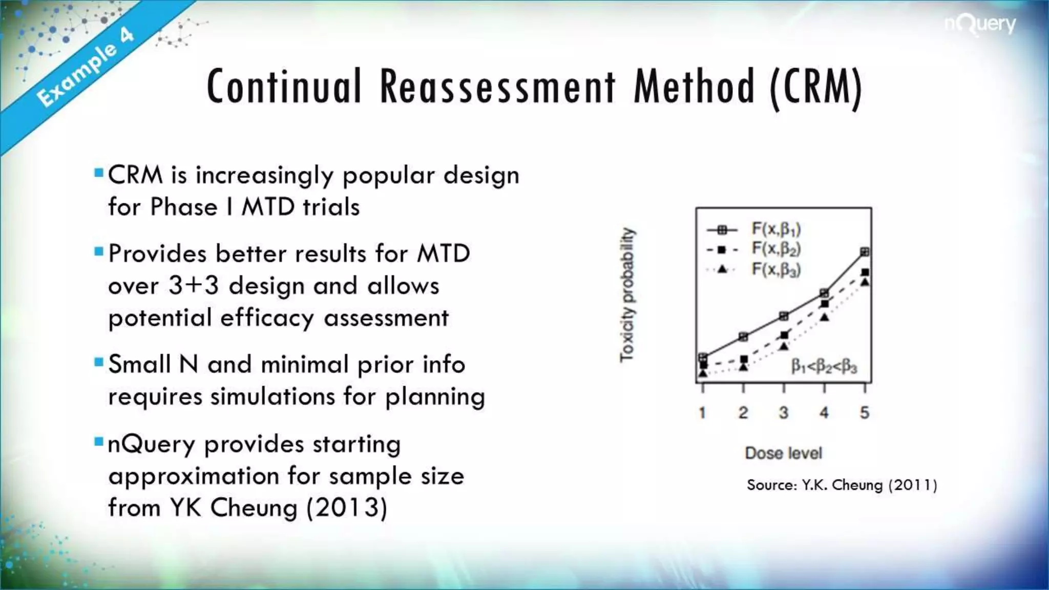
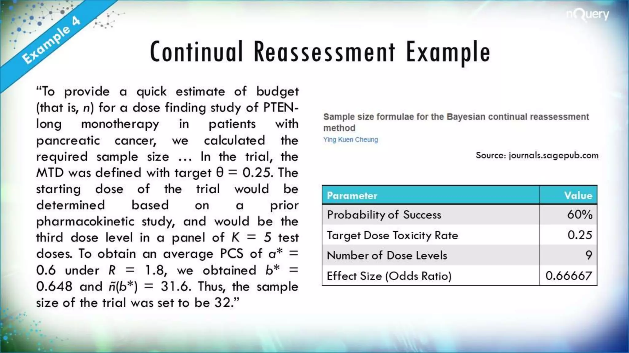
The document discusses the importance of sample size determination (SSD) in statistical studies and outlines innovative methods and challenges in SSD, particularly for clinical trials. It emphasizes various statistical techniques such as Bayesian methods and Mendelian randomization, providing examples and worked calculations to illustrate these concepts. The webinar highlights the evolution of SSD approaches, with a focus on adapting to new study designs and statistical requirements.

2.  Head of Statistics
 FDA Guest Speaker
 nQuery Lead Researcher
 Guest Lecturer
Demo Host
HOSTED BY:
Ronan
Fitzpatrick

3. Webinar Overview
Introducing Sample Size
Determination
Innovation in Sample Size
Determination
Worked nQuery Advanced Examples
Discussion and Conclusions

4. Worked Examples Overview
Mendelian Randomization
Negative Binomial Regression
Bayesian Assurance for Survival
Continual Reassessment
Method (CRM)
WORKED EXAMPLES

5. PART I
Introducing
Sample Size
Determination

6. Sample Size Determination
(SSD) Review
SSD finds the appropriate sample size for
your study
 Common metrics are statistical power, interval
width or cost
SSD seeks to balance ethical and practical
issues
 A standard design requirement for regulatory
purposes
SSD is crucial to arrive at valid conclusions in
a study

7. 𝑧 =
𝑥1 − 𝑥2 𝑛
𝑠 2
1
𝛿 =
𝜇1 − 𝜇2
𝜎
2
𝑃𝑜𝑤𝑒𝑟 = 1 − 𝛽 = 𝑃 𝑧 > 𝑧1−𝛼 𝐻1 3
= 𝑃 𝑧 −
𝛿 𝑛
2
> 𝑧1−𝛼 −
𝛿 𝑛
2
|𝐻1 4
𝑧 −
𝛿 𝑛
2
~ 𝑁 0,1 5
1 − 𝛽 = 1 − 𝛷 𝑧1−𝛼 −
𝛿 𝑛
2
6
𝑧1−𝛽 =
𝛿 𝑛
2
− 𝑧1−𝛼 7
𝑛 =
2 𝑧1−𝛽 + 𝑧1−𝛼
2
𝛿2
8

8. 5 Essential Steps for Sample Size
1 Plan Study
Study question, primary outcome,
method
2 Specify Parameters
Significance Level, Standard deviation,
dispersion
3 Choose Effect Size
Expected/targeted difference, ratio or
effect size
4
Compute Sample Sample Size for specified metric such as

9. PART 2
Innovation in
Sample Size
Determination

10. Sample Size Innovation
Overview
Sample Size Determination (SSD) has multiple
challenges to getting the appropriate sample
size.
These include uncertainty at planning stage
and lack of methods for newer statistical
methods and study designs.
In this webinar focus on three main areas of
interest:
1. Sample Size for Innovative Study Designs
2. Sample Size for Innovative Statistical Methods

11. Sample Size Innovation
Examples
1. Sample Size for Innovative Study Designs
Examples: Adaptive/seamless designs and causal
studies
2. Sample Size for Innovative Statistical
Methods
Examples: Bayesian methods, mixed and
generalized models
3. Innovative Methods in Sample Size
Determination

12. PART 3
Worked Examples

13. In 2017, 90% of organizations with clinical trials
approved
by the FDA used nQuery for sample size and power
calculation

14. nQuery Timeline
nTerim introduced
G.S.T
C.R.T
Count Data
MANOVA / ANOVA
Launch of nQuery
Advanced
New platform = Modern
all-in-one software
solution
New Bayesian Module
Survival Focus
IQ/OQ Tools
52 new Core
Tables
20 new Bayes
Tables
-Launch of nQuery
Advisor 1.0
Developed by Dr.
Janet D. Elashoff
-Contiguous
Innovation and
releases
2007 - 2016 2017 Spring 20181996-2007

15. nQuery Spring 2018 Update
Initial release focused on Survival & Bayesian tables.
April release adds 72 new tables in following areas:
New Bayes tables in
April update
New tables in April
update
Epidemiology Non-inferiority/
Equivalence
Correlation/ROC
Bayesian
Sample Size

16. Mendelian Randomization Studies
Mendelian Randomization
(MR) uses underlying
genetic variation to make
causal inferences
Uses genes with well
understood link between
polymorphism(s) and
relevant intermediate
phenotype
Note that gene must be
indirectly related to
exposure of interest
MR uses gene(s) as an
Source: S. Burgess et. al.
(2012)

17. Mendelian Randomization Example
“We computed F statistics
and R 2 values (the proportion of
variation in height and BMI
explained by the genetic risk
score) from the linear regression
to evaluate the strength of the
genetic risk score instruments in
a population of men at increased
risk of cancer. We had 82 and
78 % power to detect an odds
ratio of 1.12 and 1.25 for the
effects of height and BMI on
prostate cancer risk, assuming a
sample size of 41,062 and that
the genetic risk scores explained
6.31 and 1.46 % of the variation
Source: Springer.com
Parameter Value
Significance Level (Two-
Sided)
0.05
Positive Outcome
Proportion
0.5
Odds Ratio 1.12/1.25
Variance Explained 0.0631/0.01
46

18. Sample Size for Incidence Rates
(Counts)
Incidences rates (a.k.a
counts) are a study outcome
where measuring rate of
event per unit time
Traditional methods were
normal approximations or
Poisson model
Negative Binomial or Quasi-
Poisson model increasingly
popular
Sample Size methods for NB
and Q-P being actively
Source: R. Lehr
(1992)
Source: H. Zhu & H. Lakkis
(2014)
Source: Y. Tang (2015)

19. Negative Binomial Regression
Example
“On the basis of previous
studies of fluticasone
propionate–salmeterol
combinations we assumed a
yearly exacerbation rate with
vilanterol of 1·4 and a
dispersion parameter of 0·7.
Thus, we calculated that a
sample size of 390 assessable
patients per group in each
study would provide each study
with 90% power to detect a 25%
reduction in exacerbations in
the fluticasone furoate and
vilanterol groups versus the
Source: TheLancet.com
Parameter Value
Significance Level (Two-Sided) 0.05
Control Incidence Rate (per year) 1.4
Rate Ratio 0.75
Exposure Time (Years) 0.7
Dispersion Parameter 74
Power (%) 90%

20. Assurance for Clinical Trials
Assurance (a.k.a “Bayesian
Power”) is the unconditional
probability of significance
given a prior
Focus on methods proposed
by O’Hagan et al. (2005)
Assurance is the expectation
of the power averaged over
a prior distribution for the
effect
Often framed the “true
probability of success” of a
trial
Can be considered as a
Bayesian analogue to
Source: O’Hagan
(2005)

21. Survival Assurance Example
“Using an unstratified log-rank test at
the one-sided 2.5% significance level, a
total of 282 events would allow 92.6%
power to demonstrate a 33% risk
reduction (hazard ratio for RAD/placebo
of about 0.67, as calculated from an
anticipated 50% increase in median PFS,
from 6 months in placebo arm to 9
months in the RAD001 arm). With a
uniform accrual of approximately 23
patients per month over 74 weeks and a
minimum follow up of 39 weeks, a total
of 352 patients would be required to
obtain 282 PFS events, assuming an
exponential progression-free survival
distribution with a median of 6 months
in the Placebo arm and of 9 months in
RAD001 arm. With an estimated 10% lost
to follow up patients, a total sample size
of 392 patients should be randomized.”
Source: nejm.org
Parameter Value
Significance Level (One-Sided) 0.025
Placebo Median Survival
(months)
6
Everolimus Median Survival
(months)
9
Hazard Ratio 0.6666
7
Accrual Period (Weeks) 74
Minimum Follow-Up (Weeks) 39

22. Continual Reassessment Method
(CRM)
CRM is increasingly popular
design for Phase I MTD trials
Provides better results for
MTD over 3+3 design and
allows potential efficacy
assessment
Small N and minimal prior
info requires simulations for
planning
nQuery provides starting
approximation for sample
size from YK Cheung (2013)
Source: Y.K. Cheung
(2011)

23. Continual Reassessment Example
“To provide a quick estimate of
budget (that is, n) for a dose
finding study of PTEN-long
monotherapy in patients with
pancreatic cancer, we calculated
the required sample size … In the
trial, the MTD was defined with
target θ = 0.25. The starting dose
of the trial would be determined
based on a prior pharmacokinetic
study, and would be the third dose
level in a panel of K = 5 test doses.
To obtain an average PCS of a* =
0.6 under R = 1.8, we obtained b*
= 0.648 and ñ(b*) = 31.6. Thus,
the sample size of the trial was set
Source:
journals.sagepub.com
Parameter Value
Probability of Success 60%
Target Dose Toxicity Rate 0.25
Number of Dose Levels 9
Effect Size (Odds Ratio) 0.6666
7

24. PART 4
Discussion &
Conclusions

25. Discussion and Conclusions
Much Interest in finding SSD solutions for
new methods
 Push to allow more innovation in study planning
and design
Continuing interest in dealing with complex
SSD issues
 Uncertainty is intrinsic part of SSD since at
planning stage
Large eco-system of potential solutions for
your study

26. Q&A
Any Questions?
For further details,
contact at:
info@statsols.com
Thanks for listening!

27. References
Burgess, S. (2014). Sample size and power calculations in Mendelian randomization with a single
instrumental variable and a binary outcome. International Journal of Epidemiology, 43, 922-929
Davies, N. M., et. al. (2015). The effects of height and BMI on prostate cancer incidence and mortality: a
Mendelian randomization study in 20,848 cases and 20,214 controls from the PRACTICAL consortium.
Cancer Causes & Control, 26(11), 1603-1616.
Tang, Y. (2017). Sample size for comparing negative binomial rates in noninferiority and equivalence trials
with unequal follow-up times. Journal of biopharmaceutical statistics, 1-17.
Dransfield, M. T., et. al. (2013). Once-daily inhaled fluticasone furoate and vilanterol versus vilanterol only
for prevention of exacerbations of COPD: two replicate double-blind, parallel-group, randomised
controlled trials. The lancet Respiratory medicine, 1(3), 210-223.
O'Hagan, A., Stevens, J. W., & Campbell, M. J. (2005). Assurance in clinical trial design. Pharmaceutical
Statistics, 4(3), 187-201.
Yao, J. C., et. al. (2011). Everolimus for advanced pancreatic neuroendocrine tumors. New England Journal
of Medicine, 364(6), 514-523.
Kuen Cheung, Y. (2013), Sample size formulae for the Bayesian continual reassessment method, Clinical
Trials: Journal of the Society for Clinical Trials, 10(6), 852-861.