Download as PDF, PPTX
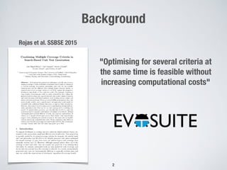
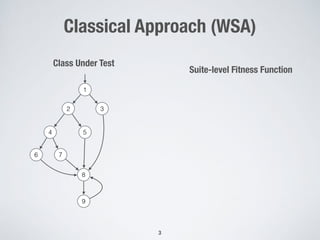
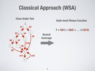

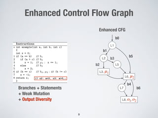
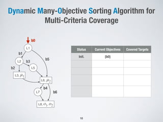
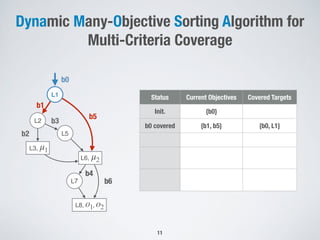
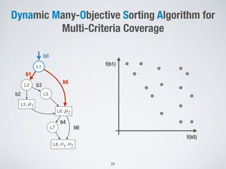
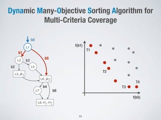

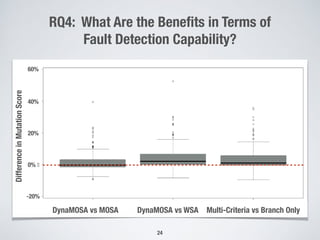

The document presents a method for many-criteria test case generation using incremental control dependency frontier exploration, optimizing several criteria simultaneously without increasing computational costs. It discusses the enhancements over classical approaches through dynamic many-objective sorting algorithms that address multi-criteria coverage effectively. Empirical studies demonstrate the proposed method's superiority in branch coverage and fault detection capabilities over traditional approaches.