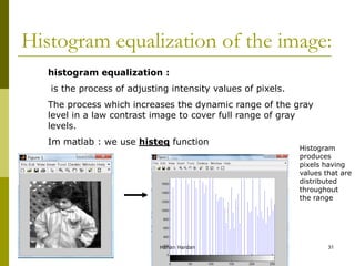
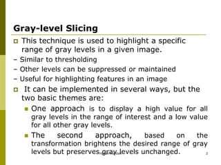
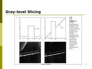
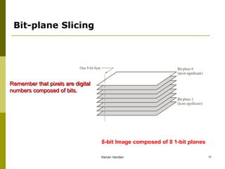
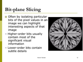
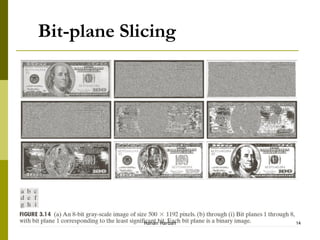
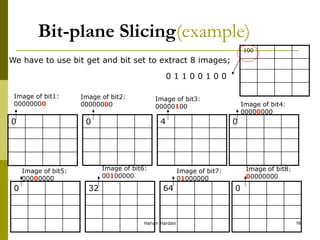
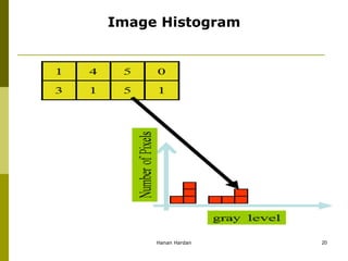
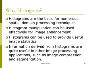
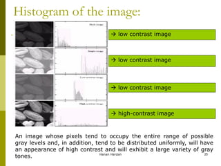
Gray-level slicing is a technique used to highlight a specific range of gray levels in an image. There are two main approaches: 1) display the range of interest as white and other levels as black, and 2) brighten the range of interest while preserving other levels. Bit-plane slicing works similarly but highlights the contribution of each bit that makes up pixel values. Histograms provide a graphical representation of pixel intensity distributions in an image and are useful for image enhancement, statistics, and other processing tasks like compression and segmentation. Histogram equalization increases contrast by spreading out the most frequent intensity values.

1. Image Processing
Chapter(3)
Part 3:Intensity Transformation and
spatial filters
Prepared by: Hanan Hardan
Hanan Hardan 1

2. Gray-level Slicing
 This technique is used to highlight a specific
range of gray levels in a given image.
– Similar to thresholding
– Other levels can be suppressed or maintained
– Useful for highlighting features in an image
 It can be implemented in several ways, but the
two basic themes are:
 One approach is to display a high value for all
gray levels in the range of interest and a low value
for all other gray levels.
 The second approach, based on the
transformation brightens the desired range of gray
levels but preserves gray levels unchanged.
Hanan Hardan 2

3. Gray-level Slicing
display in one value(e.g white) all
the values in the range of interest ,
and in another (e.g black) all other
intensities
Brightens or darkens the
desired range of intensities
but leaves all other intensity
levels in the image unchanged
Highlighting a specific range of intensities in an image.
Approach 1 Approach 2
Hanan Hardan 3

4. Gray-level Slicing
Hanan Hardan 4

5. Gray-level Slicing: approach 1
example: apply intensity level slicing in Matlab to read
cameraman image , then If the pixel intensity in the old image
is between (100  200) convert it in the new image into 255
(white). Otherwise convert it to 0 (black).
Hanan Hardan 5

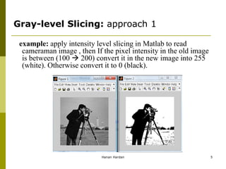
6. Gray-level Slicing: approach 1
Solution:
x=imread('cameraman.tif');
y=x;
[w h]=size(x);
for i=1:w
for j=1:h
if x(i,j)>=100 && x(i,j)<=200 y(i,j)=255;
else y(i,j)=0;
end
end
end
figure, imshow(x);
figure, imshow(y);
Hanan Hardan 6

7. example: apply intensity level slicing in Matlab to read
cameraman image , then If the pixel intensity in the old image
is between (100  200) convert it in the new image into 255
(white). Otherwise it leaves it the same.
Gray-level Slicing: approach 2
Hanan Hardan 7

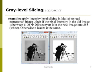
8. Gray-level Slicing: approach 2
Solution:
x=imread('cameraman.tif');
y=x;
[w h]=size(x);
for i=1:w
for j=1:h
if x(i,j)>=100 && x(i,j)<=200 y(i,j)=255;
else y(i,j)=x(i,j);
end
end
end
figure, imshow(x);
figure, imshow(y);
Hanan Hardan 8

9. example: apply intensity level slicing (approch2) in Matlab to
read moon image , then If the pixel intensity in the old image
is between (0  20) convert it in the new image into 130.
Gray-level Slicing
Homework
Hanan Hardan 9

10. Bit-plane Slicing
 Pixels are digital numbers, each one composed of
bits. Instead of highlighting gray-level range, we
could highlight the contribution made by each bit.
 This method is useful and used in image
compression.
 Most significant bits contain the majority of
visually significant data.
Hanan Hardan 10

11. Remember that pixels are digital
numbers composed of bits.
8-bit Image composed of 8 1-bit planes
Bit-plane Slicing
Hanan Hardan 11

12. Bit-plane Slicing
 Often by isolating particular
bits of the pixel values in an
image we can highlight
interesting aspects of that
image
– Higher-order bits usually
contain most of the
significant visual
information
– Lower-order bits contain
subtle details
Hanan Hardan 12

13. Bit-Plane Slicing
Hanan Hardan 13

14. Bit-plane Slicing
Hanan Hardan 14

15. Bit-Plane Slicing
Hanan Hardan 15

16. Bit-plane Slicing(example)
We have to use bit get and bit set to extract 8 images;
100
0 1 1 0 0 1 0 0
0 0 4 0
0 32 64 0
Image of bit1:
00000000
Image of bit2:
00000000
Image of bit3:
00000100 Image of bit4:
00000000
Image of bit5:
00000000
Image of bit6:
00100000
Image of bit7:
01000000
Image of bit8:
00000000
Hanan Hardan 16

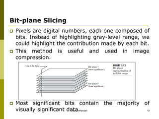
17. Bit-plane Slicing- programmed
example: apply bit-plane slicing in Matlab to read cameraman
image , then extract the image of bit 6.
Solution:
x=imread('cameraman.tif');
y=x*0;
[w h]=size(x);
for i=1:w
for j=1:h
b=bitget(x(i,j),6);
y(i,j)=bitset(y(i,j),6,b);
end
end
figure, imshow(x);
figure, imshow(y);
Hanan Hardan 17

18. Histogram Processing
What is a Histogram?
 In Statistics, Histogram is a graphical
representation showing a visual
impression of the distribution of data.
 An Image Histogram is a type of
histogram that acts as a graphical
representation of the lightness/color
distribution in a digital image. It plots the
number of pixels for each value.
Hanan Hardan 18

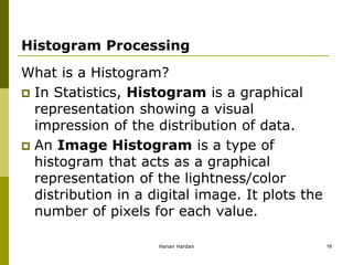
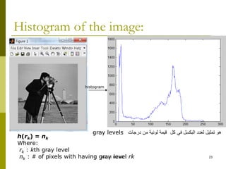
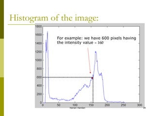
19. Histogram?
 The histogram of a digital image with gray
levels in the range [0, L-1] is a discrete
function:
h(rk) = nk
Where:
rk : kth gray level
nk : # of pixels with having gray level rk
Hanan Hardan 19

20. Image Histogram
Hanan Hardan 20

21. Histogram Processing
 It is common practice to normalize a
histogram by dividing each of its values by
the total number of pixels in the image,
denoted by n. Thus, a normalized
histogram is given by
p(rk) = nk / n, for k = 0, 1, …, L -1.
 Thus, p(rk) gives an estimate of the
probability of occurrence of gray level rk.
 Note that the sum of all components of a
normalized histogram is equal to 1.
Hanan Hardan 21

22. Why Histogram?
 Histograms are the basis for numerous
spatial domain processing techniques
 Histogram manipulation can be used
effectively for image enhancement
 Histograms can be used to provide useful
image statistics
 Information derived from histograms are
quite useful in other image processing
applications, such as image compression
and segmentation.
Hanan Hardan 22

23. Histogram of the image:
histogram
h(rk) = nk
Where:
rk : kth gray level
nk : # of pixels with having gray level rk
‫كل‬ ‫في‬ ‫البكسل‬ ‫لعدد‬ ‫تمثيل‬ ‫هو‬
‫درجات‬ ‫من‬ ‫لونية‬ ‫قيمة‬
gray levels
Hanan Hardan 23

24. Histogram of the image:
For example: we have 600 pixels having
the intensity value ≈ 160
Hanan Hardan 24

25. Histogram of the image:
 low contrast image
 low contrast image
 low contrast image
 high-contrast image
An image whose pixels tend to occupy the entire range of possible
gray levels and, in addition, tend to be distributed uniformly, will have
an appearance of high contrast and will exhibit a large variety of gray
tones. Hanan Hardan 25

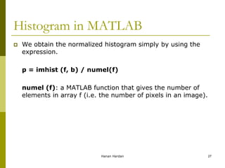
26. Histogram in MATLAB
h = imhist (f, b)
Where f, is the input image, h is the histogram, b is number
of bins (tick marks) used in forming the histogram (b = 255
is the default)
A bin, is simply, a subdivision of the intensity scale. For
example, if we are working with uint8 images and we let b
= 2, then the intensity scale is subdivided into two ranges:
0 – 127 and 128 – 255. the resulting histograms will have
two values: h(1) equals to the number of pixels in the
image with values in the interval [0,127], and h(2) equal to
the number of pixels with values in the interval [128 255].
Hanan Hardan 26

27. Histogram in MATLAB
 We obtain the normalized histogram simply by using the
expression.
p = imhist (f, b) / numel(f)
numel (f): a MATLAB function that gives the number of
elements in array f (i.e. the number of pixels in an image).
Hanan Hardan 27

28. Other ways to display Histograms
 Consider an image f. The simplest way to plot its histogram
is to use imhist with no output specified:
>> imhist (f);
Figure 3.7(a) shows the result.
Hanan Hardan 28

29. Other ways to display Histograms
 A stem graph
 A bar graph
 A Plot graph
>> h = imhist(f);
>> bar (h);
>> plot (h);
>> stem (h);
Hanan Hardan 29

30. Histogram equalization of the image:
We have this image in matlab called
pout.tif, when we plot its histogram it
is showed like this:
Notice that the
pixels intensity
values are
concentrated on
the middle
(low contrast)
Hanan Hardan 30

31. Histogram equalization of the image:
histogram equalization :
is the process of adjusting intensity values of pixels.
The process which increases the dynamic range of the gray
level in a law contrast image to cover full range of gray
levels.
Im matlab : we use histeq function
Histogram
produces
pixels having
values that are
distributed
throughout
the range
Hanan Hardan 31

32. Histogram equalization of the image:
Notice that histogram
equalization does not
always produce a
good result
Hanan Hardan 32

33. Equalization (mathematically)
g(x) = (L/n). T(X) -1
Where,
G(X) : the new image after equalization
L: No of gray levels 2n
n: No of pixels
T(x): cumulative sum of each gray level
Hanan Hardan 33

34. Equalization (mathematically)
G(x)
T(X)
‫تراكمي‬ ‫مجموع‬
‫للبكسل‬
X
‫لكل‬ ‫البكسل‬ ‫عدد‬
Graylevel
L
grayl
evels
0
1
1
0
0
4
3
1
1
9
5
2
2
15
6
3
4
21
6
4
5
27
6
5
6
29
2
6
7
32
3
7
Assume that we have
(3bits per pixels) or 8
levels of grayscale,
and we want to
equalize the following
image example.
G(x)=(L/n). T(X) -1
=(8/32). T(x) -1
No of pixels
‫الكلي‬ ‫البكسالت‬ ‫عدد‬
8 ‫ال‬ ‫عدد‬
graylevel
Hanan Hardan 34