Computer Vision(Histograms and Point Operations )

1. Computer Vision(CSEN5233)
Histograms and Point Operations
(Part 1)
Prof. Jhalak Dutta
Computer Science &Engineering Dept.
Heritage Institute of Technology, Kolkata(HITK)

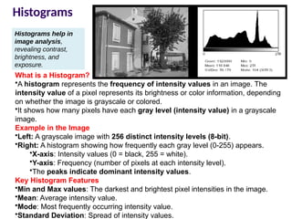
2. Histograms
What is a Histogram?
•A histogram represents the frequency of intensity values in an image. The
intensity value of a pixel represents its brightness or color information, depending
on whether the image is grayscale or colored.
•It shows how many pixels have each gray level (intensity value) in a grayscale
image.
Example in the Image
•Left: A grayscale image with 256 distinct intensity levels (8-bit).
•Right: A histogram showing how frequently each gray level (0-255) appears.
•X-axis: Intensity values (0 = black, 255 = white).
•Y-axis: Frequency (number of pixels at each intensity level).
•The peaks indicate dominant intensity values.
Key Histogram Features
•Min and Max values: The darkest and brightest pixel intensities in the image.
•Mean: Average intensity value.
•Mode: Most frequently occurring intensity value.
•Standard Deviation: Spread of intensity values.
Histograms help in
image analysis,
revealing contrast,
brightness, and
exposure.

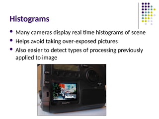
3. Histograms
 Many cameras display real time histograms of scene
 Helps avoid taking over exposed
‐ pictures
 Also easier to detect types of processing previously
applied to image

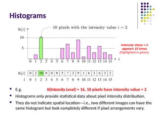
4. Histograms
 E.g. K(Intensity Level) = 16, 10 pixels have intensity value = 2
 Histograms only provide statistical data about pixel intensity distribution.
 They do not indicate spatial location—i.e., two different images can have the
same histogram but look completely different if pixel arrangements vary.
Intensity Value = 2
appears 10 times
(highlighted in green).

5. Histograms
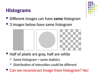
 Different images can have same histogram
 3 images below have same histogram
 Half of pixels are gray, half are white
 Same histogram = same statisics
 Distribution of intensities could be different
 Can we reconstruct image from histogram? No!

6. Histograms
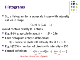
 So, a histogram for a grayscale image with intensity
values in range
would contain exactly K entries
 E.g. 8 bit
‐ grayscale image, K = 28 = 256
 Each histogram entry is defined as:
h(i) = number of pixels with intensity i for all 0 < i < K.
 E.g: h(255) = number of pixels with intensity = 255
 Formal definition
Number (size of set) of pixels

7. Interpreting Histograms
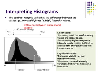
 The contrast range is defined by the difference between the
darkest (a_low) and lightest (a_high) intensity values.
Difference between darkest and
lightest
Linear Scale:
•Commonly used, but low-frequency
values are harder to see.
•Dominated by higher-frequency
intensity levels, making it difficult to
analyze dark or bright details with
low occurrences.
Logarithmic Scale:
•Enhances visibility of low-
frequency values.
•Helps analyze small intensity
variations that may be hidden in a
linear scale.

8. Histograms
 Histograms help detect image acquisition issues
 Problems with image can be identified on histogram
 Over and under exposure
 Brightness
 Contrast
 Dynamic Range
 Point operations can be used to alter histogram. E.g
 Addition
 Multiplication
 Exp and Log
 Intensity Windowing (Contrast Modification)

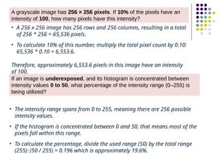
9. A grayscale image has 256 × 256 pixels. If 10% of the pixels have an
intensity of 100, how many pixels have this intensity?
• A 256 x 256 image has 256 rows and 256 columns, resulting in a total
of 256 * 256 = 65,536 pixels.
• To calculate 10% of this number, multiply the total pixel count by 0.10:
65,536 * 0.10 = 6,553.6.
Therefore, approximately 6,553.6 pixels in this image have an intensity
of 100.
If an image is underexposed, and its histogram is concentrated between
intensity values 0 to 50, what percentage of the intensity range (0–255) is
being utilized?
• The intensity range spans from 0 to 255, meaning there are 256 possible
intensity values.
• If the histogram is concentrated between 0 and 50, that means most of the
pixels fall within this range.
• To calculate the percentage, divide the used range (50) by the total range
(255): (50 / 255) = 0.196 which is approximately 19.6%.

10. If an image has pixel values in the range [50, 200], and we apply a
transformation I' = I + 20, what will be the new intensity range?
New intensity range after addition (I' = I + 20): [70, 220].
Given an image with intensity range [30, 200], a windowing function maps [50,
150] to [0, 255]. What is the new intensity of a pixel originally at 75 using linear
scaling?

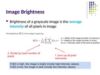
11. Image Brightness
 Brightness of a grayscale image is the average
intensity of all pixels in image
1. Sum up all pixel
intensities
2. Divide by total number of
pixels
If B(I) is high, the image is bright (mostly high-intensity values).
If B(I) is low, the image is dark (mostly low-intensity values).
w = Width of the image (number of columns).
h = Height of the image (number of rows).
I(u,v) = Intensity value of the pixel at position

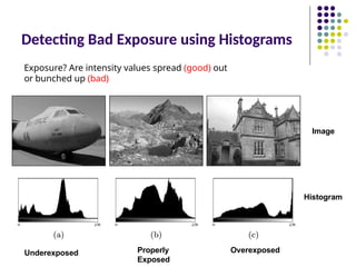
13. Detecting Bad Exposure using Histograms
Underexposed Overexposed
Properly
Exposed
Exposure? Are intensity values spread (good) out
or bunched up (bad)
Histogram
Image

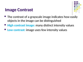
14. Image Contrast
 The contrast of a grayscale image indicates how easily
objects in the image can be distinguished
 High contrast image: many distinct intensity values
 Low contrast: image uses few intensity values

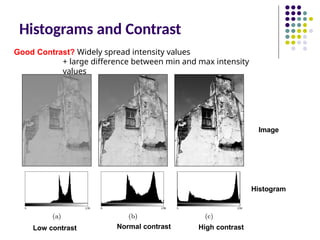
15. Histograms and Contrast
Low contrast High contrast
Normal contrast
Good Contrast? Widely spread intensity values
+ large difference between min and max intensity
values
Histogram
Image

16. Contrast Equation?

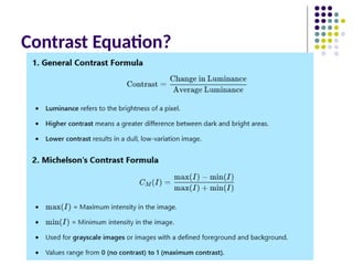
17. Histograms and Dynamic Range
 Dynamic Range is the number of distinct intensity values
present in an image.
 Difficult to increase image dynamic range
 HDR (High Dynamic Range) Imaging: Typically uses 12-14 bits per pixel to capture a wider
intensity range. These images are later downsampled to 8-bit for standard displays.
High Dynamic Range Extremely low
Dynamic Range
(6 intensity
values)
Low Dynamic Range
(64 intensities)
•Higher dynamic
range → More shades
of gray → Better
image quality.
•Low dynamic range
→ Posterization and
loss of details.

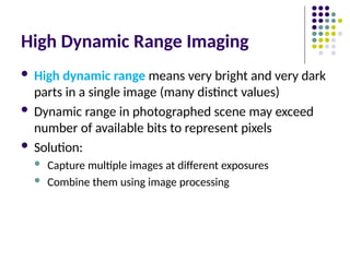
18. High Dynamic Range Imaging
 High dynamic range means very bright and very dark
parts in a single image (many distinct values)
 Dynamic range in photographed scene may exceed
number of available bits to represent pixels
 Solution:
 Capture multiple images at different exposures
 Combine them using image processing

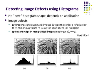
19. Detecting Image Defects using Histograms
 No “best” histogram shape, depends on application
 Image defects
 Saturation: scene illumination values outside the sensor’s range are set
to its min or max values => results in spike at ends of histogram
 Spikes and Gaps in manipulated images (not original). Why?
Next Slide

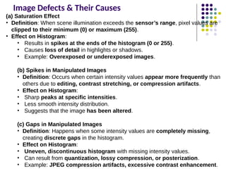
20. Image Defects & Their Causes
(a) Saturation Effect
• Definition: When scene illumination exceeds the sensor’s range, pixel values are
clipped to their minimum (0) or maximum (255).
• Effect on Histogram:
• Results in spikes at the ends of the histogram (0 or 255).
• Causes loss of detail in highlights or shadows.
• Example: Overexposed or underexposed images.
(b) Spikes in Manipulated Images
• Definition: Occurs when certain intensity values appear more frequently than
others due to editing, contrast stretching, or compression artifacts.
• Effect on Histogram:
• Sharp peaks at specific intensities.
• Less smooth intensity distribution.
• Suggests that the image has been altered.
(c) Gaps in Manipulated Images
• Definition: Happens when some intensity values are completely missing,
creating discrete gaps in the histogram.
• Effect on Histogram:
• Uneven, discontinuous histogram with missing intensity values.
• Can result from quantization, lossy compression, or posterization.
• Example: JPEG compression artifacts, excessive contrast enhancement.

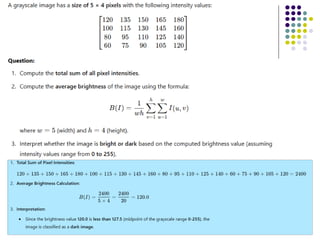
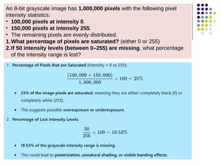
21. An 8-bit grayscale image has 1,000,000 pixels with the following pixel
intensity statistics:
• 100,000 pixels at intensity 0.
• 150,000 pixels at intensity 255.
• The remaining pixels are evenly distributed.
1.What percentage of pixels are saturated? (either 0 or 255)
2.If 50 intensity levels (between 0–255) are missing, what percentage
of the intensity range is lost?

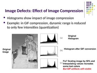
22. Image Defects: Effect of Image Compression
 Histograms show impact of image compression
 Example: in GIF compression, dynamic range is reduced
to only few intensities (quantization)
Original
Image
Original
Histogram
Histogram after GIF conversion
Fix? Scaling image by 50% and
Interpolating values recreates
some lost colors
But GIF artifacts still visible

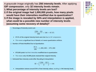
23. A grayscale image originally has 256 intensity levels. After applying
GIF compression, only 32 intensity levels remain.
1.What percentage of intensity levels are lost?
2.If the original image had 1,000,000 pixels, how many pixels
would have their intensities modified due to quantization?
3.If the image is rescaled by 50% and interpolation is applied,
what could be a possible new number of intensity levels
(assuming some recovery of details)?

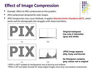
24. Effect of Image Compression
 Example: Effect of JPEG compression on line graphics
 JPEG compression designed for color images
 JPEG Compression Uses Lossy Methods. It applies Discrete Cosine Transform (DCT), which
works well for photographs but struggles with sharp transitions.
Original histogram
has only 2 intensities
(gray and white)
JPEG image appears
dirty, fuzzy and blurred
Its Histogram contains
gray values not in original
•JPEG is NOT suitable for text/graphics due to blurring and artifacts.
•PNG or GIF are better formats for sharp-edged images since they use lossless compression.

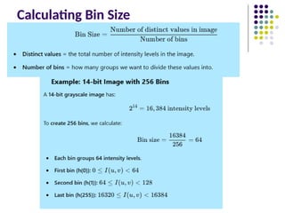
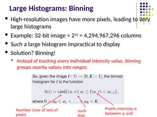
25. Large Histograms: Binning
 High-resolution images have more pixels, leading to very
large histograms
 Example: 32 bit
‐ image = 232 = 4,294,967,296 columns
 Such a large histogram impractical to display
 Solution? Binning!
 Instead of tracking every individual intensity value, binning
groups nearby values into ranges.
Number (size of set) of
pixels
such
that
Pixel’s intensity is
between ai and

26. Calculating Bin Size

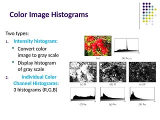
28. Color Image Histograms
Two types:
1. Intensity histogram:
 Convert color
image to gray scale
 Display histogram
of gray scale
2. Individual Color
Channel Histograms:
3 histograms (R,G,B)

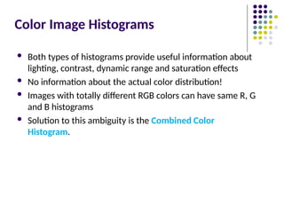
29. Color Image Histograms
 Both types of histograms provide useful information about
lighting, contrast, dynamic range and saturation effects
 No information about the actual color distribution!
 Images with totally different RGB colors can have same R, G
and B histograms
 Solution to this ambiguity is the Combined Color
Histogram.

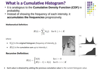
30. What is a Cumulative Histogram?
• It is analogous to the Cumulative Density Function (CDF) in
probability.
• Instead of showing the frequency of each intensity, it
accumulates the frequencies progressively.

31. Clamping
Why Clamping is Needed?
• Some image processing operations (like filtering, contrast stretching,
or gamma correction) can produce pixel values outside the standard
range.
• Values greater than 255 (in 8-bit images) need to be capped at
255.
• Values less than 0 should be clamped to 0.
 Function below will clamp (force) all values to fall within range
[a,b]
Clamping is a method used in image processing to ensure that pixel
values remain within a valid intensity range (e.g., [0,255] for an 8-bit
image).

32. Inverting Images
Image inversion is a process where the pixel intensities of an image are
reversed, producing a negative of the original image. This is commonly used
in image processing to enhance visibility in certain scenarios, such as medical
imaging and artistic effects.
 2 steps
1. Multiple intensity by 1
‐ , This
flips the values.
2. Add constant (e.g. amax) to
put result in valid range
[0,amax]
Original Inverted Image
Where:
• Amax is the maximum intensity
value (255 for an 8-bit
grayscale image).
• 𝑎 is the original intensity value.
• finvert(a) is the inverted intensity
value.

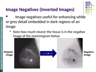
33. Image Negatives (Inverted Images)
 Image negatives useful for enhancing white
or grey detail embedded in dark regions of an
image
 Note how much clearer the tissue is in the negative
image of the mammogram below
s = 1.0 - r
Original
Image
Negative
Image
Images
taken
from
Gonzalez
&
Woods,
Digital
Image
Processing
(2002)

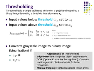
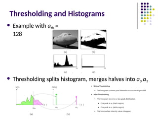
34. Thresholding
Thresholding is a simple technique to convert a grayscale image into a
binary image by setting a threshold intensity value ath​
.
Applications of Thresholding
• Edge Detection: Simplifies object segmentation.
• OCR (Optical Character Recognition): Converts
text images into black-and-white for better
recognition.
• Medical Imaging: Highlights specific tissue areas.

35. Thresholding Example

36. Thresholding and Histograms
 Example with ath =
128
 Thresholding splits histogram, merges halves into a0 a1

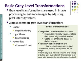
37. Basic Grey Level Transformations
Gray level transformations are used in image
processing to enhance images by adjusting
pixel intensity values.
3 most common gray level transformation:
 Linear
 Negative/Identity
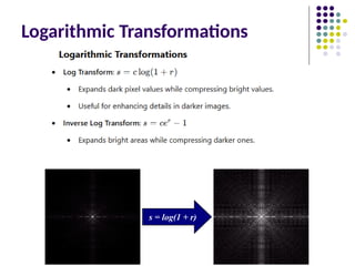
 Logarithmic
 Log/Inverse log
 Power law
 nth power/nth root
Images
taken
from
Gonzalez
&
Woods,
Digital
Image
Processing
(2002)
Linear Transformations
 Negative Transformation: s=L−1−r
• Inverts the intensity values, making
dark areas bright and vice versa.
• Useful for enhancing details in
darker regions.
 Identity Transformation: s=r
Leaves the image unchanged.
L= Maximum intensity value(255 for a 8 bit
image)
r= Input gray level intensity (original pixel value).
s=Output gray level intensity (transformed pixel
value after applying the transformation function).

38. Logarithmic Transformations
s = log(1 + r)

39. Power Law Transformations
 Map narrow range of dark input values into wider
range of output values or vice versa
Images
taken
from
Gonzalez
&
Woods,
Digital
Image
Processing
(2002)

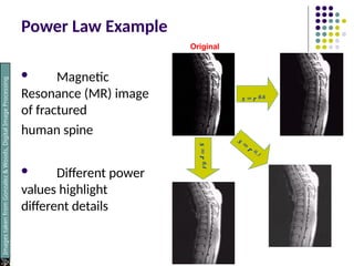
40. Power Law Example
 Magnetic
Resonance (MR) image
of fractured
human spine
 Different power
values highlight
different details
s = r 0.6
s
=
r
0.4
Images
taken
from
Gonzalez
&
Woods,
Digital
Image
Processing
(2002)
Original

41. Intensity Windowing ?

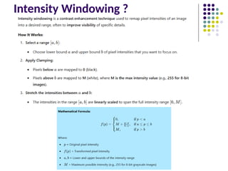
42. Intensity Windowing Example
Contrasts
easier to
see
Use Cases:
1. Medical Imaging (CT/MRI/X-ray scans)
Enhances the visibility of soft tissues or bones by selecting a specific range of pixel intensities.
2. Satellite & Thermal Imaging
Focuses on specific intensity ranges to detect heat signatures, land cover changes, or objects.
3. Image Processing for Object Detection
Helps in identifying objects by emphasizing relevant intensity ranges.

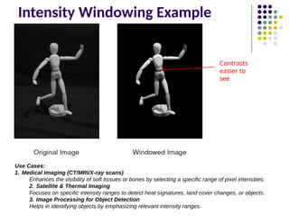
43. Point Operations and Histograms
 Effect of some point operations easier to observe on histograms
 Increasing brightness
 Raising contrast
 Inverting image
 Point operations only shift, merge histogram entries
 Operations that merge histogram bins are irreversible
Combining
histogram operation
easier to observe on
histogram

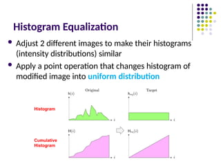
44. Histogram Equalization
 Adjust 2 different images to make their histograms
(intensity distributions) similar
 Apply a point operation that changes histogram of
modified image into uniform distribution
Histogram
Cumulative
Histogram

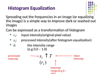
45. Histogram Equalization
Spreading out the frequencies in an image (or equalizing
the image) is a simple way to improve dark or washed out
images
Can be expressed as a transformation of histogram
 rk: input intensity(original pixel value)
 sk: processed intensity(after histogram equalization)
 k: the intensity range
(e.g 0.0 – 1.0)
sk  T
(rk )
input
intensity
processed
intensity
Intensity
range (e.g 0 –

46. Equalization Transformation Function
Images
taken
from
Gonzalez
&
Woods,
Digital
Image
Processing
(2002)
Most pixel intensities are clustered in
a place
The histogram after
equalization spreads the pixel
intensities more evenly.