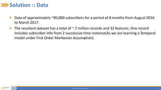
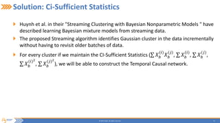
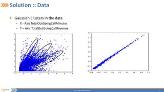
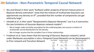
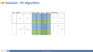
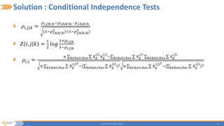
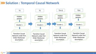
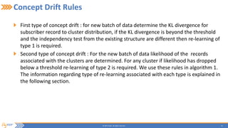
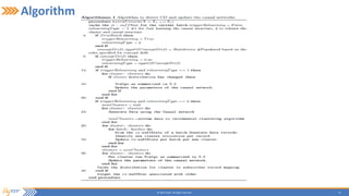
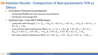
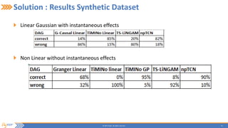
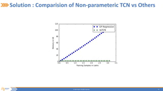
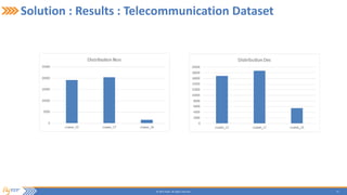
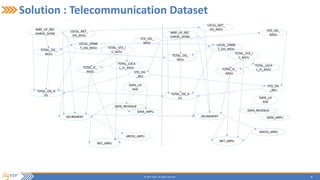
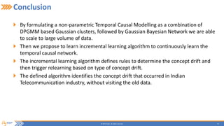
7th International Conference on Pattern Recognition and Machine
Intelligence
Dec 5-8th, ISI Kolkata
Incremental Learning of Non-Stationary Temporal
Causal Networks for Telecommunication Domain
Ram Mohan
R&D Department, Flytxt, Trivandrum, India
Santanu Chaudhury
CEERI, Pilani, India
Brejesh Lall
Department of Electrical Engineering, Indian Institute of Technology, Delhi, India
2© 2015 Flytxt. All rights reserved.
Table Of Contents
Why Causal Modelling?
• Simpson’s Paradox
• Decision Making
Problem Statement Definition
• Volume of Data
• Non-Stationary Distributions
• Challenge Lies only in Structure Learning
Solution
• Data and Model
• Algorithm
• Results
3© 2015 Flytxt. All rights reserved.
Why Causal Modelling?
Simpson’s Paradox
4© 2015 Flytxt. All rights reserved.
Why Causal Modelling?
Simpson’s Paradox
Cancer
Male/Female Smoker
5© 2015 Flytxt. All rights reserved.
Why Causal Modelling?
Simpson’s Paradox – Continuous Values
6© 2015 Flytxt. All rights reserved.
Why Causal Modelling?
Churn
Recharge
MRP
Outgoing
Call Minutes
7© 2015 Flytxt. All rights reserved.
Causal Inference
Judea Pearl in her work defines structural causal modelling.
DATA
Causal Inference
Algorithms(Structure
Learning Algorithms)
8© 2015 Flytxt. All rights reserved.
Causal Model
A causal diagram is a graphical tool that enables the visualization of causal relationships
between variables in a causal model. A typical causal diagram will comprise a set of
variables (or nodes) defined as being within the scope of the model being represented.
Any variable in the diagram should be connected by an arrow to another variable with
which it has a causal influence - the arrowhead delineates the direction of this causal
relationship, e.g., an arrow connecting variables A and B with the arrowhead at B
indicates a relationship whereby (all other factors being equal) a qualitative or
quantitative change in A may cause change in B.
Causal/Bayesian Network ‘G’ is a Directed Acyclic Graph, where Probability Distribution
P factorizes according to P(X)=∏_(𝑖=1)^𝑛▒〖𝑃(𝑥_𝑖│𝑃𝑎(𝑥_𝑖 ) ),〗 P is specified as a set of
CPDs associated with G and the I(G) ⊆ I(P)
9© 2015 Flytxt. All rights reserved.
Problem Statement Definition
Causal modelling on Large Volume Non-Stationary Data in a streaming setup.
• Big Data
• Volume
• Velocity
• Variety
• Under lying Distribution
• Non-Stationary
10© 2015 Flytxt. All rights reserved.
Non-Stationary Distributions
A time-series dataset can be classified as generated from Stationary Process or Non-
Stationary Process
In statistics, a stationary process is a stochastic process whose joint probability
distribution does not change when shifted in time. Consequently, parameters such as
mean and variance, if they are present, also do not change over time.
Non-stationary process joint probability distribution undergoes change when shifted in
time. Consequently parameters such as mean and variance, if they are present, do
change over time.
Why model Non-Stationary?
• There is a shift from detection-diagnosis-mitigation of unfavorable events(anomalies) to prediction-
prognosis-prevention is seen across various engineering domains such as health care,
telecommunication, financial institutions.
• To be able to forecast we have to model Non-Stationary time series data as a machine learning
model.
11© 2015 Flytxt. All rights reserved.
Concept Drift
In predictive analytics and machine learning, the concept drift is a phenomenon a
phenomenon associated with time instance when the underlying statistical properties
of target variable actually undergoes a change.
12© 2015 Flytxt. All rights reserved.
Learning in a Non Stationary domain
Adaptive learning refers to updating predictive models online during their operation to
react to concept drifts
Have the following tasks:
• Detect concept drift
• distinguish drifts from noise and be adaptive to changes, but robust to noise
• operate in less than arrival time interval and use not more than a fixed amount of memory for any
storage
13© 2015 Flytxt. All rights reserved.
Solution :: Data
Data of approximately ~90,000 subscribers for a period of 8 months from August 2016
to March 2017.
The resultant dataset has a total of ~.7 million records and 32 features. One record
includes subscriber info from 2 successive time instance(As we are learning a Temporal
model under First Order Markovian Assumption).
14© 2015 Flytxt. All rights reserved.
Solution : Data – Feature Info
15© 2015 Flytxt. All rights reserved.
Solution: Ci-Sufficient Statistics
Huynh et al. in their "Streaming Clustering with Bayesian Nonparametric Models " have
described learning Bayesian mixture models from streaming data.
The proposed Streaming algorithm identifies Gaussian cluster in the data incrementally
without having to revisit older batches of data.
For every cluster if we maintain the CI-Sufficient Statistics ( 𝑋 𝑏
(𝑖)
𝑋 𝑏
(𝑗)
, 𝑋 𝑏
(𝑖)
, 𝑋 𝑏
(𝑗)
,
𝑋 𝑏
(𝑖)2
, 𝑋 𝑏
(𝑗)2
), we will be able to construct the Temporal Causal network.
16© 2015 Flytxt. All rights reserved.
Solution :: Data
X - Axis TotalOutGoingCallMinutes
Y – Axis TotalOutGoingCallRevenue
17© 2015 Flytxt. All rights reserved.
Solution :: Data
Gaussian Clusters in the data
• X - Axis TotalOutGoingCallMinutes
• Y – Axis TotalOutGoingCallRevenue
18© 2015 Flytxt. All rights reserved.
Solution : Non-Parametric Temporal Causal Network
Wu and Ghosal in their work “Kullback Leibler property of kernel mixture priors in
Bayesian density estimation" show that the mixture of multivariate Gaussians can
approximate any density on 𝑅 𝑑
, provided that the number of components can get
arbitrarily large”.
Ickstadt et al. in their work "Nonparametric Bayesian Networks" use it as it overcomes
the two limitations of Gaussian Bayesian network models*:
• We no longer make normality assumption for the underlying data, but assume a mixture of
multivariate normal distributions for the density.
• We no longer assume that the variables X are in linear relationships.
Friedman et al. have shown that the learning of Dynamic Bayesian network ( which
under Markovian assumption is also a Temporal Causal Network) can be decomposed in
to Prior network and Transition Network
19© 2015 Flytxt. All rights reserved.
Solution : PC-Algorithm
20© 2015 Flytxt. All rights reserved.
Solution : Conditional Independence Tests
𝜌𝑖,𝑗|𝑘 =
𝜌 𝑖,𝑗|𝑘h−𝜌 𝑖,ℎ|𝑘h ∙ 𝜌 𝑗,ℎ|𝑘h
(1−𝜌𝑖,ℎ|𝑘h
2 )∙(1−𝜌 𝑗,ℎ|𝑘h
2 )
𝑍 𝑖, 𝑗 𝑘 =
1
2
𝑙𝑜𝑔
1+𝜌 𝑖,𝑗|𝑘
1−𝜌 𝑖,𝑗|𝑘
𝜌𝑖,𝑗 =
𝑛 𝑏∈𝑏𝑎𝑡𝑐ℎ𝑒𝑠 𝑋 𝑏
(𝑖)
𝑋 𝑏
(𝑗)
− 𝑏∈𝑏𝑎𝑡𝑐ℎ𝑒𝑠 𝑋 𝑏
(𝑖)
𝑏∈𝑏𝑎𝑡𝑐ℎ𝑒𝑠 𝑋 𝑏
(𝑗)
𝑛 𝑏∈𝑏𝑎𝑡𝑐ℎ𝑒𝑠 𝑋 𝑏
(𝑖)2
−( 𝑏∈𝑏𝑎𝑡𝑐ℎ𝑒𝑠 𝑋 𝑏
(𝑖)
)2 𝑛 𝑏∈𝑏𝑎𝑡𝑐ℎ𝑒𝑠 𝑋 𝑏
(𝑗)2
−( 𝑏∈𝑏𝑎𝑡𝑐ℎ𝑒𝑠 𝑋 𝑏
(𝑗)
)2
21© 2015 Flytxt. All rights reserved.
Solution : Temporal Causal Network
22© 2015 Flytxt. All rights reserved.
Concept Drift Rules
First type of concept drift : for new batch of data determine the KL divergence for
subscriber record to cluster distribution, if the KL divergence is beyond the threshold
and the independency test from the existing structure are different then re-learning of
type 1 is required.
Second type of concept drift : For the new batch of data likelihood of the records
associated with the clusters are determined. For any cluster if likelihood has dropped
below a threshold re-learning of type 2 is required. We use these rules in algorithm 1.
The information regarding type of re-learning associated with each type is explained in
the following section.
23© 2015 Flytxt. All rights reserved.
Algorithm
24© 2015 Flytxt. All rights reserved.
Solution Results : Comparision of Non-parameteric TCN vs
Others
Formulation Temporal Causal Network
• Combining DPGMM and Linear Gaussian Causal Network
• Distributed Learning Algorithm
Synthetic Data – From NIPS TiMINo Paper:
• Confounder with time lag:𝑍𝑡 = 𝑎 ∙ 𝑍𝑡−1 + 𝑁𝑍,𝑡, 𝑋𝑡 = 0.6 ∙ 𝑋𝑡−1 + 0.5 ∙ 𝑍𝑡−1 + 𝑁𝑋,𝑡, 𝑌𝑡 = 0.6 ∙ 𝑌𝑡−1 +
0.5 ∙ 𝑍𝑡−2 + 𝑁𝑌,𝑡
• Linear Gaussian with instantaneous effects.: 𝑋𝑡 = 𝑎 ∙ 𝑋𝑡−1 + 𝑁𝑋,𝑡, 𝑊𝑡 = 0.6 ∙ 𝑊𝑡−1 + 0.5 ∙ 𝑋𝑡 +
𝑁 𝑊,𝑡, 𝑌𝑡 = 0.6 ∙ 𝑌𝑡−1 + 0.5 ∙ 𝑊𝑡−1 + 𝑁𝑌,𝑡, 𝑍𝑡 = 0.6 ∙ 𝑍𝑡−1 + 0.5 ∙ 𝑊𝑡 + 0.2 ∙ 𝑌𝑡−1 + 𝑁𝑍,𝑡
• Non Linear without instantaneous effects: 𝑋𝑡 = 0.8 ∙ 𝑋𝑡−1 + 0.3 ∙ 𝑁𝑋,𝑡, 𝑌𝑡 = 0.4 ∙ 𝑌𝑡−1 + 𝑋𝑡−1 −
25© 2015 Flytxt. All rights reserved.
Solution : Results Synthetic Dataset
Linear Gaussian with instantaneous effects
Non Linear without instantaneous effects
26© 2015 Flytxt. All rights reserved.
Solution : Comparision of Non-parameteric TCN vs Others
27© 2015 Flytxt. All rights reserved.
Solution : Results : Telecommunication Dataset
28© 2015 Flytxt. All rights reserved.
Solution : Telecommunication Dataset
29© 2015 Flytxt. All rights reserved.
Conclusion
By formulating a non-parametric Temporal Causal Modelling as a combination of
DPGMM based Gaussian clusters, followed by Gaussian Bayesian Network we are able
to scale to large volume of data.
Then we propose to learn incremental learning algorithm to continuously learn the
temporal causal network.
The incremental learning algorithm defines rules to determine the concept drift and
then trigger relearning based on type of concept drift.
The defined algorithm identifies the concept drift that occurred in Indian
Telecommunication industry, without visiting the old data.
30© 2015 Flytxt. All rights reserved.
References
Causal inference in statistics: An overview
• Judea Pearl, 2009 Statistics Survey
Incremental Learning of Nonparametric Bayesian Mixture Models:
• Ryan Gomess, Max Welling, Pietro Perona :: Computer Vision and Pattern Recognition, 2008.
Estimating High-Dimensional Directed Acyclic Graphs with the PC-Algorithm
• Markus Kalisch, Peter Buhlmann, 2007 JMLR
Order-Independent Constraint-Based Causal Structure Learning
• Diego Colombo, Marloes H. Maathuis, 2014 JMLR
Streaming Clustering with Bayesian Nonparametric Models
• Viet Huynha, Dinh Phunga, 2016 ELSEVIER
Thank You
www.flytxt.com | info@flytxt.com
© 2015 Flytxt. All rights reserved.

Ikdd co ds2017presentation_v2

  • 1.
    7th International Conferenceon Pattern Recognition and Machine Intelligence Dec 5-8th, ISI Kolkata Incremental Learning of Non-Stationary Temporal Causal Networks for Telecommunication Domain Ram Mohan R&D Department, Flytxt, Trivandrum, India Santanu Chaudhury CEERI, Pilani, India Brejesh Lall Department of Electrical Engineering, Indian Institute of Technology, Delhi, India
  • 2.
    2© 2015 Flytxt.All rights reserved. Table Of Contents Why Causal Modelling? • Simpson’s Paradox • Decision Making Problem Statement Definition • Volume of Data • Non-Stationary Distributions • Challenge Lies only in Structure Learning Solution • Data and Model • Algorithm • Results
  • 3.
    3© 2015 Flytxt.All rights reserved. Why Causal Modelling? Simpson’s Paradox
  • 4.
    4© 2015 Flytxt.All rights reserved. Why Causal Modelling? Simpson’s Paradox Cancer Male/Female Smoker
  • 5.
    5© 2015 Flytxt.All rights reserved. Why Causal Modelling? Simpson’s Paradox – Continuous Values
  • 6.
    6© 2015 Flytxt.All rights reserved. Why Causal Modelling? Churn Recharge MRP Outgoing Call Minutes
  • 7.
    7© 2015 Flytxt.All rights reserved. Causal Inference Judea Pearl in her work defines structural causal modelling. DATA Causal Inference Algorithms(Structure Learning Algorithms)
  • 8.
    8© 2015 Flytxt.All rights reserved. Causal Model A causal diagram is a graphical tool that enables the visualization of causal relationships between variables in a causal model. A typical causal diagram will comprise a set of variables (or nodes) defined as being within the scope of the model being represented. Any variable in the diagram should be connected by an arrow to another variable with which it has a causal influence - the arrowhead delineates the direction of this causal relationship, e.g., an arrow connecting variables A and B with the arrowhead at B indicates a relationship whereby (all other factors being equal) a qualitative or quantitative change in A may cause change in B. Causal/Bayesian Network ‘G’ is a Directed Acyclic Graph, where Probability Distribution P factorizes according to P(X)=∏_(𝑖=1)^𝑛▒〖𝑃(𝑥_𝑖│𝑃𝑎(𝑥_𝑖 ) ),〗 P is specified as a set of CPDs associated with G and the I(G) ⊆ I(P)
  • 9.
    9© 2015 Flytxt.All rights reserved. Problem Statement Definition Causal modelling on Large Volume Non-Stationary Data in a streaming setup. • Big Data • Volume • Velocity • Variety • Under lying Distribution • Non-Stationary
  • 10.
    10© 2015 Flytxt.All rights reserved. Non-Stationary Distributions A time-series dataset can be classified as generated from Stationary Process or Non- Stationary Process In statistics, a stationary process is a stochastic process whose joint probability distribution does not change when shifted in time. Consequently, parameters such as mean and variance, if they are present, also do not change over time. Non-stationary process joint probability distribution undergoes change when shifted in time. Consequently parameters such as mean and variance, if they are present, do change over time. Why model Non-Stationary? • There is a shift from detection-diagnosis-mitigation of unfavorable events(anomalies) to prediction- prognosis-prevention is seen across various engineering domains such as health care, telecommunication, financial institutions. • To be able to forecast we have to model Non-Stationary time series data as a machine learning model.
  • 11.
    11© 2015 Flytxt.All rights reserved. Concept Drift In predictive analytics and machine learning, the concept drift is a phenomenon a phenomenon associated with time instance when the underlying statistical properties of target variable actually undergoes a change.
  • 12.
    12© 2015 Flytxt.All rights reserved. Learning in a Non Stationary domain Adaptive learning refers to updating predictive models online during their operation to react to concept drifts Have the following tasks: • Detect concept drift • distinguish drifts from noise and be adaptive to changes, but robust to noise • operate in less than arrival time interval and use not more than a fixed amount of memory for any storage
  • 13.
    13© 2015 Flytxt.All rights reserved. Solution :: Data Data of approximately ~90,000 subscribers for a period of 8 months from August 2016 to March 2017. The resultant dataset has a total of ~.7 million records and 32 features. One record includes subscriber info from 2 successive time instance(As we are learning a Temporal model under First Order Markovian Assumption).
  • 14.
    14© 2015 Flytxt.All rights reserved. Solution : Data – Feature Info
  • 15.
    15© 2015 Flytxt.All rights reserved. Solution: Ci-Sufficient Statistics Huynh et al. in their "Streaming Clustering with Bayesian Nonparametric Models " have described learning Bayesian mixture models from streaming data. The proposed Streaming algorithm identifies Gaussian cluster in the data incrementally without having to revisit older batches of data. For every cluster if we maintain the CI-Sufficient Statistics ( 𝑋 𝑏 (𝑖) 𝑋 𝑏 (𝑗) , 𝑋 𝑏 (𝑖) , 𝑋 𝑏 (𝑗) , 𝑋 𝑏 (𝑖)2 , 𝑋 𝑏 (𝑗)2 ), we will be able to construct the Temporal Causal network.
  • 16.
    16© 2015 Flytxt.All rights reserved. Solution :: Data X - Axis TotalOutGoingCallMinutes Y – Axis TotalOutGoingCallRevenue
  • 17.
    17© 2015 Flytxt.All rights reserved. Solution :: Data Gaussian Clusters in the data • X - Axis TotalOutGoingCallMinutes • Y – Axis TotalOutGoingCallRevenue
  • 18.
    18© 2015 Flytxt.All rights reserved. Solution : Non-Parametric Temporal Causal Network Wu and Ghosal in their work “Kullback Leibler property of kernel mixture priors in Bayesian density estimation" show that the mixture of multivariate Gaussians can approximate any density on 𝑅 𝑑 , provided that the number of components can get arbitrarily large”. Ickstadt et al. in their work "Nonparametric Bayesian Networks" use it as it overcomes the two limitations of Gaussian Bayesian network models*: • We no longer make normality assumption for the underlying data, but assume a mixture of multivariate normal distributions for the density. • We no longer assume that the variables X are in linear relationships. Friedman et al. have shown that the learning of Dynamic Bayesian network ( which under Markovian assumption is also a Temporal Causal Network) can be decomposed in to Prior network and Transition Network
  • 19.
    19© 2015 Flytxt.All rights reserved. Solution : PC-Algorithm
  • 20.
    20© 2015 Flytxt.All rights reserved. Solution : Conditional Independence Tests 𝜌𝑖,𝑗|𝑘 = 𝜌 𝑖,𝑗|𝑘h−𝜌 𝑖,ℎ|𝑘h ∙ 𝜌 𝑗,ℎ|𝑘h (1−𝜌𝑖,ℎ|𝑘h 2 )∙(1−𝜌 𝑗,ℎ|𝑘h 2 ) 𝑍 𝑖, 𝑗 𝑘 = 1 2 𝑙𝑜𝑔 1+𝜌 𝑖,𝑗|𝑘 1−𝜌 𝑖,𝑗|𝑘 𝜌𝑖,𝑗 = 𝑛 𝑏∈𝑏𝑎𝑡𝑐ℎ𝑒𝑠 𝑋 𝑏 (𝑖) 𝑋 𝑏 (𝑗) − 𝑏∈𝑏𝑎𝑡𝑐ℎ𝑒𝑠 𝑋 𝑏 (𝑖) 𝑏∈𝑏𝑎𝑡𝑐ℎ𝑒𝑠 𝑋 𝑏 (𝑗) 𝑛 𝑏∈𝑏𝑎𝑡𝑐ℎ𝑒𝑠 𝑋 𝑏 (𝑖)2 −( 𝑏∈𝑏𝑎𝑡𝑐ℎ𝑒𝑠 𝑋 𝑏 (𝑖) )2 𝑛 𝑏∈𝑏𝑎𝑡𝑐ℎ𝑒𝑠 𝑋 𝑏 (𝑗)2 −( 𝑏∈𝑏𝑎𝑡𝑐ℎ𝑒𝑠 𝑋 𝑏 (𝑗) )2
  • 21.
    21© 2015 Flytxt.All rights reserved. Solution : Temporal Causal Network
  • 22.
    22© 2015 Flytxt.All rights reserved. Concept Drift Rules First type of concept drift : for new batch of data determine the KL divergence for subscriber record to cluster distribution, if the KL divergence is beyond the threshold and the independency test from the existing structure are different then re-learning of type 1 is required. Second type of concept drift : For the new batch of data likelihood of the records associated with the clusters are determined. For any cluster if likelihood has dropped below a threshold re-learning of type 2 is required. We use these rules in algorithm 1. The information regarding type of re-learning associated with each type is explained in the following section.
  • 23.
    23© 2015 Flytxt.All rights reserved. Algorithm
  • 24.
    24© 2015 Flytxt.All rights reserved. Solution Results : Comparision of Non-parameteric TCN vs Others Formulation Temporal Causal Network • Combining DPGMM and Linear Gaussian Causal Network • Distributed Learning Algorithm Synthetic Data – From NIPS TiMINo Paper: • Confounder with time lag:𝑍𝑡 = 𝑎 ∙ 𝑍𝑡−1 + 𝑁𝑍,𝑡, 𝑋𝑡 = 0.6 ∙ 𝑋𝑡−1 + 0.5 ∙ 𝑍𝑡−1 + 𝑁𝑋,𝑡, 𝑌𝑡 = 0.6 ∙ 𝑌𝑡−1 + 0.5 ∙ 𝑍𝑡−2 + 𝑁𝑌,𝑡 • Linear Gaussian with instantaneous effects.: 𝑋𝑡 = 𝑎 ∙ 𝑋𝑡−1 + 𝑁𝑋,𝑡, 𝑊𝑡 = 0.6 ∙ 𝑊𝑡−1 + 0.5 ∙ 𝑋𝑡 + 𝑁 𝑊,𝑡, 𝑌𝑡 = 0.6 ∙ 𝑌𝑡−1 + 0.5 ∙ 𝑊𝑡−1 + 𝑁𝑌,𝑡, 𝑍𝑡 = 0.6 ∙ 𝑍𝑡−1 + 0.5 ∙ 𝑊𝑡 + 0.2 ∙ 𝑌𝑡−1 + 𝑁𝑍,𝑡 • Non Linear without instantaneous effects: 𝑋𝑡 = 0.8 ∙ 𝑋𝑡−1 + 0.3 ∙ 𝑁𝑋,𝑡, 𝑌𝑡 = 0.4 ∙ 𝑌𝑡−1 + 𝑋𝑡−1 −
  • 25.
    25© 2015 Flytxt.All rights reserved. Solution : Results Synthetic Dataset Linear Gaussian with instantaneous effects Non Linear without instantaneous effects
  • 26.
    26© 2015 Flytxt.All rights reserved. Solution : Comparision of Non-parameteric TCN vs Others
  • 27.
    27© 2015 Flytxt.All rights reserved. Solution : Results : Telecommunication Dataset
  • 28.
    28© 2015 Flytxt.All rights reserved. Solution : Telecommunication Dataset
  • 29.
    29© 2015 Flytxt.All rights reserved. Conclusion By formulating a non-parametric Temporal Causal Modelling as a combination of DPGMM based Gaussian clusters, followed by Gaussian Bayesian Network we are able to scale to large volume of data. Then we propose to learn incremental learning algorithm to continuously learn the temporal causal network. The incremental learning algorithm defines rules to determine the concept drift and then trigger relearning based on type of concept drift. The defined algorithm identifies the concept drift that occurred in Indian Telecommunication industry, without visiting the old data.
  • 30.
    30© 2015 Flytxt.All rights reserved. References Causal inference in statistics: An overview • Judea Pearl, 2009 Statistics Survey Incremental Learning of Nonparametric Bayesian Mixture Models: • Ryan Gomess, Max Welling, Pietro Perona :: Computer Vision and Pattern Recognition, 2008. Estimating High-Dimensional Directed Acyclic Graphs with the PC-Algorithm • Markus Kalisch, Peter Buhlmann, 2007 JMLR Order-Independent Constraint-Based Causal Structure Learning • Diego Colombo, Marloes H. Maathuis, 2014 JMLR Streaming Clustering with Bayesian Nonparametric Models • Viet Huynha, Dinh Phunga, 2016 ELSEVIER
  • 31.
    Thank You www.flytxt.com |info@flytxt.com © 2015 Flytxt. All rights reserved.