Download to read offline
![International Journal of Engineering and Technical Research (IJETR)
ISSN: 2321-0869 (O) 2454-4698 (P), Volume-5, Issue-3, July 2016
108 www.erpublication.org
Abstract— Present article deals with the reflection of
wave’s incident at the surface of transversely isotropic
micropolar visco elastic medium under the theory of
thermoelasticity of type-II and type-III. The wave equations are
solved by imposing proper conditions on components of
displacement, stresses and temperature distribution. It is found
that there exist four different waves viz., quasi-longitudinal
displacement(qLD)wave, quasi transverse
displacement(qTD)wave, quasi transverse microrotational
(qTM)wave and quasi thermal wave (qT). Amplitude ratio of
these reflected waves are presented, when different waves are
incident. Numerically simulated results have been depicted
graphically for different angle of incidence with respect to
frequency. Some special cases of interest also have been
deduced form the present investigation.
Index Terms—Micropolar, Reflection, Amplitude Ratios,
Viscoelastic.
I. INTRODUCTION
Depending upon the mechanical properties, the materials
of earth have been classified as elastic, viscoelastic, sandy,
granular, microstructure etc. Some parts of earth may
supposed to be composed of material possessing
micropolar/granular structure instead of continuous elastic
materials. To explain the fundamental departure of
microcontinuum theories from the classical continuum
theories, the former is a continuum model embedded with
microstructures to describe the microscopic motion or a
non-local model to describe the long range material
interaction. This extends the application of the continuum
model to microscopic space and short-time scales.
Material is endowed with microstructure, like atoms
and molecules at microscopic scale, grains and fibers or
particulate at mesoscopic scale. Homogenization of a
basically heterogeneous material depends on scale of interest.
When stress fluctuation is small enough compared to
microstructure of material, homogenization can be made
without considering the detailed microstructure of the
material. However, if it is not the case, the microstructure of
material must be considered properly in a homogenized
formulation [1], [2]. The concept of microcontinuum,
proposed by Eringen [1], can take into account the
microstructure of material while the theory itself remains still
Manuscript received June 09, 2016.
Rajani Rani Gupta, Department of Mathematics & Applied Sciences,
Middle East College, Muscat, Oman, (e-mail: dr.rajanigupta@gmail.com).
Raj Rani Gupta, Department of CS & IT, Mazoon College, Muscat,
Oman, (e-mail: raji.mmec@gmail.com).
in a continuum formulation. The first grade microcontinuum
consist a hierarachy of theories, such as, micropolar,
microstretch and micromorphic, depending on how much
micro-degrees of freedom is incorporated. These
microcontinuum theories are believed to be potential tools to
characterize the behavior of material with complicated
microstructures.
The most popular microcontinuum theory is micropolar one,
in this theory, a material point can still be considered as
infinitely small, however, there are microstructures inside of
this point. So there are two sets of variable to describe the
deformation of this material point, one characterizes the
motion of the inertia center of this material point; the other
describes the motion of the microstructure inside of this point.
In micropolar theory, the motion of the microstructure is
supposed to be an independently rigid rotation. Application
of this theory can be found in [1] and [3].
Recently, the theory of thermoelasticity without energy
dissipation, which provides sufficient basic modifications to
the constitutive equation to permit the treatment of a much
wider class of flow problems, has been proposed by Green
and Naghdi [4] (called the GN theory). The discussion
presented in the above reference includes the derivation of a
complete set of governing equations of the linearized version
of the theory for homogeneous and isotropic materials in
terms of displacement and temperature fields and a proof of
the uniqueness of the solution of the corresponding initial
mixed boundary value problem. Chandrasekharaiah and
Srinath [5] investigated one-dimensional wave propagation
in the context of the GN theory.
The aim of the present paper is to study the
reflection of waves in transversely isotropic micropolar
viscoelastic medium under the theory of thermoelasticity of
type-II and type-III. The propagation of waves in micropolar
materials has many applications in various fields of science
and technology, namely, atomic physics, industrial
engineering, thermal power plants, submarine structures,
pressure vessel, aerospace, chemical pipes and metallurgy.
The graphical representation in given for amplitude ratios of
various reflected waves for different incident waves at
different angle of incidence i.e. for 𝜃 = 30 𝑜
, 45 𝑜
𝑎𝑛𝑑 90 𝑜
.
II. BASIC EQUATIONS
The basic equations in dynamic theory of the plain strain of a
homogeneous, transversely isotropic micropolar viscoelastic
Plane wave reflection in micropolar transversely
isotropic thermo-visco-elastic half space under GN
type-II and type-III
Rajani Rani Gupta, Raj Rani Gupta](https://image.slidesharecdn.com/ijetr042201-200501112726/85/Ijetr042201-1-320.jpg)
![International Journal of Engineering and Technical Research (IJETR)
ISSN: 2321-0869 (O) 2454-4698 (P), Volume-5, Issue-3, July 2016
108 www.erpublication.org
Abstract— Present article deals with the reflection of
wave’s incident at the surface of transversely isotropic
micropolar visco elastic medium under the theory of
thermoelasticity of type-II and type-III. The wave equations are
solved by imposing proper conditions on components of
displacement, stresses and temperature distribution. It is found
that there exist four different waves viz., quasi-longitudinal
displacement(qLD)wave, quasi transverse
displacement(qTD)wave, quasi transverse microrotational
(qTM)wave and quasi thermal wave (qT). Amplitude ratio of
these reflected waves are presented, when different waves are
incident. Numerically simulated results have been depicted
graphically for different angle of incidence with respect to
frequency. Some special cases of interest also have been
deduced form the present investigation.
Index Terms—Micropolar, Reflection, Amplitude Ratios,
Viscoelastic.
I. INTRODUCTION
Depending upon the mechanical properties, the materials
of earth have been classified as elastic, viscoelastic, sandy,
granular, microstructure etc. Some parts of earth may
supposed to be composed of material possessing
micropolar/granular structure instead of continuous elastic
materials. To explain the fundamental departure of
microcontinuum theories from the classical continuum
theories, the former is a continuum model embedded with
microstructures to describe the microscopic motion or a
non-local model to describe the long range material
interaction. This extends the application of the continuum
model to microscopic space and short-time scales.
Material is endowed with microstructure, like atoms
and molecules at microscopic scale, grains and fibers or
particulate at mesoscopic scale. Homogenization of a
basically heterogeneous material depends on scale of interest.
When stress fluctuation is small enough compared to
microstructure of material, homogenization can be made
without considering the detailed microstructure of the
material. However, if it is not the case, the microstructure of
material must be considered properly in a homogenized
formulation [1], [2]. The concept of microcontinuum,
proposed by Eringen [1], can take into account the
microstructure of material while the theory itself remains still
Manuscript received June 09, 2016.
Rajani Rani Gupta, Department of Mathematics & Applied Sciences,
Middle East College, Muscat, Oman, (e-mail: dr.rajanigupta@gmail.com).
Raj Rani Gupta, Department of CS & IT, Mazoon College, Muscat,
Oman, (e-mail: raji.mmec@gmail.com).
in a continuum formulation. The first grade microcontinuum
consist a hierarachy of theories, such as, micropolar,
microstretch and micromorphic, depending on how much
micro-degrees of freedom is incorporated. These
microcontinuum theories are believed to be potential tools to
characterize the behavior of material with complicated
microstructures.
The most popular microcontinuum theory is micropolar one,
in this theory, a material point can still be considered as
infinitely small, however, there are microstructures inside of
this point. So there are two sets of variable to describe the
deformation of this material point, one characterizes the
motion of the inertia center of this material point; the other
describes the motion of the microstructure inside of this point.
In micropolar theory, the motion of the microstructure is
supposed to be an independently rigid rotation. Application
of this theory can be found in [1] and [3].
Recently, the theory of thermoelasticity without energy
dissipation, which provides sufficient basic modifications to
the constitutive equation to permit the treatment of a much
wider class of flow problems, has been proposed by Green
and Naghdi [4] (called the GN theory). The discussion
presented in the above reference includes the derivation of a
complete set of governing equations of the linearized version
of the theory for homogeneous and isotropic materials in
terms of displacement and temperature fields and a proof of
the uniqueness of the solution of the corresponding initial
mixed boundary value problem. Chandrasekharaiah and
Srinath [5] investigated one-dimensional wave propagation
in the context of the GN theory.
The aim of the present paper is to study the
reflection of waves in transversely isotropic micropolar
viscoelastic medium under the theory of thermoelasticity of
type-II and type-III. The propagation of waves in micropolar
materials has many applications in various fields of science
and technology, namely, atomic physics, industrial
engineering, thermal power plants, submarine structures,
pressure vessel, aerospace, chemical pipes and metallurgy.
The graphical representation in given for amplitude ratios of
various reflected waves for different incident waves at
different angle of incidence i.e. for 𝜃 = 30 𝑜
, 45 𝑜
𝑎𝑛𝑑 90 𝑜
.
II. BASIC EQUATIONS
The basic equations in dynamic theory of the plain strain of a
homogeneous, transversely isotropic micropolar viscoelastic
Plane wave reflection in micropolar transversely
isotropic thermo-visco-elastic half space under GN
type-II and type-III
Rajani Rani Gupta, Raj Rani Gupta](https://image.slidesharecdn.com/ijetr042201-200501112726/75/Ijetr042201-1-2048.jpg)
![Plane wave reflection in micropolar transversely isotropic thermo-visco-elastic half space under GN type-II and
type-III
109 www.erpublication.org
medium following Eringen [1] and Green and Naghdi [4] in
the theory of thermoelasticity of type-II and type-III in
absence of body forces, body couples and heat sources are
given by:
Balance laws
ijij ut , (1)
kijijkiik jtm , , (2)
Heat conduction equation
klklklklklkl u
t
T
t
T
cTTK ,2
2
02
2
*
,,
*
(3)
The constitutive relations can be given as:
𝑡 𝑘𝑙 = 𝐴 𝑘𝑙𝑚𝑛 𝐸 𝑚𝑛 + 𝐺 𝑘𝑙𝑚𝑛Ψ 𝑚𝑛 − 𝛽𝑘𝑙 𝑇,
𝑚 𝑘𝑙 = 𝐴𝑙𝑘𝑚𝑛 𝐸 𝑚𝑛 + 𝐺 𝑚𝑛𝑙𝑘Ψ 𝑚𝑛 (4)
Where
𝐴𝑖𝑗𝑘𝑙 = 𝐴′𝑖𝑗𝑘𝑙 + 𝐴′′𝑖𝑗𝑘𝑙
𝜕
𝜕𝑡
,
𝐵𝑖𝑗𝑘𝑙 = 𝐵′𝑖𝑗𝑘𝑙 + 𝐵′′𝑖𝑗𝑘𝑙
𝜕
𝜕𝑡
,
𝐺𝑖𝑗𝑘𝑙 = 𝐺′𝑖𝑗𝑘𝑙 + 𝐺′′𝑖𝑗𝑘𝑙
𝜕
𝜕𝑡
,
deformation and wryness tensor are defined by
klklmlkmklkl ue ,, ,
,
(5)
In these relations, we have used the following notations: is
the density, lkm permutation symbol, 𝑢𝑖 components of
displacement vector, i components of microrotation vector,
𝑡 𝑘𝑙 components of the stress tensor, 𝑚 𝑘𝑙 components of the
couple stress tensor, kle components of micropolar strain
tensor, kl are the characteristic constants of the theory,
*
c
is specific heat at constant strain, *
klK is the thermal
conductivity, 𝛽𝑘𝑙 = 𝐴 𝑘𝑙𝑚𝑛 𝛼 𝑚𝑛 are the thermal elastic
coupling tensor, 𝛼 𝑚𝑛 are the coefficient of linear thermal
expansion.
III. FORMULATION OF THE PROBLEM
In present case we consider homogeneous, transversely
isotropic micropolar viscoelastic medium under the theory of
thermoelasticity of type-II and type-III, initially in an
undeformed state and at uniform temperature 𝑇𝑜. We take the
origin of coordinate system on the plane surface with 𝑥3 axis
pointing normally into the half-space, which is thus
represented by 𝑥3 > 0. We restricted our analysis to the two
dimensional problem by assuming the displacement vector 𝑢⃗
and microrotation vector 𝜙⃗ as
𝑢⃗ = (𝑢1, 0, 𝑢3), 𝜙⃗ = (0, 𝜙2, 0) (6)
With the aid of equation (6), the field equations (1)-(4)
for transversely isotropic micropolar viscoelastic medium
under the theory of thermoelasticity of type-II and type-III
reduce to:
,
)(
2
1
2
1
1
3
2
1
31
3
2
56132
3
1
2
552
1
1
2
11
t
u
x
T
x
K
xx
u
AA
x
u
A
x
u
A
(7)
,
)(
2
3
2
3
3
1
2
2
31
1
2
56132
3
3
2
332
1
3
2
66
t
u
x
T
x
K
xx
u
AA
x
u
A
x
u
A
(8)
,2
2
2
3
3
1
3
1
122
3
2
2
662
1
2
2
77
tx
u
K
x
u
KX
x
B
x
B
(9)
),(
3
3
3
1
1
12
2
2
2
*
2
3
2
2
*
32
1
2
2
*
12
3
2
2
32
1
2
2
1
x
u
x
u
t
T
t
T
C
tx
K
tx
K
xx
o
(10)
where
311256662
5556133313133131111
,,,
,,,
KKXAAK
AAKAAAA
are the coefficients of linear thermal expansion and we have
used the notations 11 → 1, 33 → 3, 12 → 7, 13 → 6, 23 → 4
for the material constants.
For simplification we use the following
non-dimensional variables:
,'
L
x
x i
i ,'
L
u
u i
i ,
1
'
o
ij
ij
T
t
t
,
1
'
o
ij
ij
TL
m
m
,
1
112'
2
oT
A
0
'
T
T
T ,' 1
t
L
c
t .112
1
A
c
(11)
where L is a parameter having dimension of length and 𝑐1is
the longitudinal wave velocity of the medium.
IV. SOLUTION OF THE PROBLEM
Let 𝑝(𝑝1, 0, 𝑝3) denote the unit propagation vector of the
plane waves propagating in 𝑥1 𝑥3-plane.
We seek plane wave solution of the equations of motion of
the form
)(
231231
3311
),,,(),,,( ctxpxpi
eTuuTuu
(12)
where and k are respectively the phase velocity and the
wave number the components ),,,( 231 Tuu define the
amplitude and polarization of particle displacement,
microrotation and temperature distribution in the medium.
With the help of equations (11) and (12) in equations
(7)-(10), we get four homogeneous equations in four
unknowns. Solving the resultant system of equations for](https://image.slidesharecdn.com/ijetr042201-200501112726/85/Ijetr042201-2-320.jpg)
![International Journal of Engineering and Technical Research (IJETR)
ISSN: 2321-0869 (O) 2454-4698 (P), Volume-5, Issue-3, July 2016
112 www.erpublication.org
𝐵44 = 𝐵′
44(1 + 𝑖 𝜔 𝑅7
−1), 𝐵66 = 𝐵′
66(1 + 𝑖 𝜔 𝑅8
−1),
where
𝑅1
−1
= 8.05, 𝑅2
−1
= 2, 𝑅3
−1
= 1.05, 𝑅4
−1
= 4.05,
𝑅5
−1
= 2.05, 𝑅6
−1
= 7.05, 𝑅7
−1
= 2.05, 𝑅8
−1
= 4.05
Following Gauthier [6] we take, the non-dimensional
values for Aluminium epoxy like composite as
,/1049.1,/1089.1
,/1059.7,/1019.2
2929
2933
mNKmN
mNmKg
,10196.0 24
mj
,sec/107.1 2*
CmJK o
KCalC /04.1*
, .1063.2 5
N
Graphical representation is given for the variations of
amplitude ratios of reflected qLD, qTD, qTM and qT waves
when four types of waves viz. qLD, qTD, qTM and qT waves
are incident at the free surface to compare the results in two
cases, one for the waves incident from transversely isotropic
micropolar medium under the theory of thermoelasticity of
type-II and type-III (MTIWED) and other from micropolar
transversely isotropic viscoelastic material with energy
dissipation (MVWED). In figures 1-4, the graphical
representation is given for variations of amplitude ratios
21 , ZZ , 3Z and 4Z for incident qLD wave. Figures 5-8,
9-12 and 13-16, respectively show the similar state in case of
incident qTD, qTM, and qT waves. Here 21 , ZZ , 3Z and
4Z are, respectively, the amplitude ratios of reflected qLD,
qTD, qTM and qT wave.
These variations are shown for three different angle of
incidence viz., 𝜃 = 30 𝑜
, 45 𝑜
𝑎𝑛𝑑 90 𝑜
. In these figures the
solid lines corresponds to the case of MTIWED while the
dotted lines corresponds to the case of MVWED. Also, the
solid lines without center symbol, lines with center symbol
(−0 − 0 −), solid lines with center symbol (− × − ×
−), respectively, represent variations for 𝜃 = 30 𝑜
, 𝜃 =
45 𝑜
and 𝜃 = 90 𝑜
in case on MTIWED, whereas the
corresponding broken lines represent the same condition in
the case of MVWED.
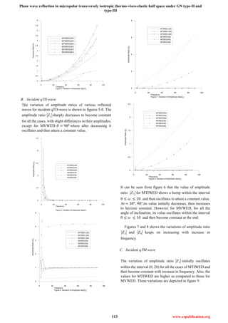
A. Incident qLD wave
It is observed from figure 1 that the amplitude ratio 1Z of
reflected qLD-wave first increases sharply to peak value and
then decreases sharply to attain a constant value, when
𝜃 = 45 𝑜
for MTIWED. While, for all the other cases, its
value initially increase and then oscillate to become constant
ultimately.
0 20 40 60 80 100
Frequency
Figure 1. Variation of Amplitude ratio |Z1|
0
0.1
0.2
0.3
0.4
0.5
0.6
0.7
0.8
0.9
1
1.1
1.2
1.3
AmplitudeRatio|Z1|
MTIWED(30o
)
MTIWED(45o)
MTIWED(90o
)
MVWED(30o)
MVWED(45o
)
MVWED(90o)
0 20 40 60 80 100
Frequency
Figure 2. Variation of Amplitude ratio|Z2|
0
10
20
30
40
50
AmplitudeRatio|Z2|
MTIWED(30o
)
MTIWED(45o
)
MTIWED(90o
)
MVWED(30o
)
MVWED(45o
)
MVWED(90o
)
Figure 2, 3 and 4 indicate the variations of amplitude
ratio 2Z , 3Z and 4Z of reflected qTD-wave which
shows that for all the cases, the value of 2Z , 3Z and
4Z initially oscillate with very small amplitude and then
steadily increases with increase in frequency, for all the
three angles of inclination.
0 20 40 60 80 100
Frequency
Figure 3. Variation of Amplitude ratio|Z3|
0
1.5
3
4.5
6
7.5
9
10.5
12
13.5
15
16.5
AmplitudeRation|Z3|
MTIWED(30o)
MTIWED(45o)
MTIWED(90o
)
MVWED(30o)
MVWED(45o
)
MVWED(90o)](https://image.slidesharecdn.com/ijetr042201-200501112726/85/Ijetr042201-5-320.jpg)
![Plane wave reflection in micropolar transversely isotropic thermo-visco-elastic half space under GN type-II and
type-III
115 www.erpublication.org
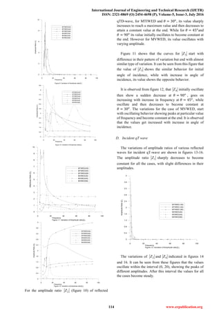
0 20 40 60 80 100
Frequency
Figure 14. Variation of Amplitude ratio|Z2|
0
5
10
15
20
25
30
35
AmplitudeRatio|Z2|
MTIWED (30)
MTIWED (45)
MTIWED (90)
MVWED(30)
MVWED(45)
MVWED(90)
0 20 40 60 80 100
Frequency
Figure 15. Variation of Amplitude ratio|Z3|
0
10
20
30
40
50
AmplitudeRatio|Z3|
MTIWED(30)
MTIWED(45)
MTIWED(90)
MVWED(30)
MVWED(45)
MVWED(90)
0 20 40 60 80 100
Frequency
Figure 16. Variation of Amplitude ratio|Z4|
0
0.5
1
1.5
2
2.5
3
3.5
4
AmplitudeRatio|Z4|
MTIWED(30)
MTIWED(45)
MTIWED(90)
MVWED(30)
MVWED(45)
MVWED(90)
Variations in the values of 3Z indicate that viscoelasticity as
well as angle of incidence show a significant impact on it
throughout the whole range (figure 15). The behavior of 3Z
oscillatory, within the range 0 ≤ 𝜔 ≤ 20 . The values of
maximum with amplitude ratio 3Z first increase from small
values to small oscillations and ultimately decrease to
become steady. The values for MVWED are higher as
compared to those for MVWED at 𝜃 = 30 𝑜
𝑎𝑛𝑑 45 𝑜
, but the
behavior is reversed with further increase in the angle of
incidence. Viscoelasticity show a greater impact on iZ ,
i=1,2,3,4 as compared to the angle of incidence.
VIII. CONCLUSION
The analytic expressions of amplitude ratios for various
reflected waves are obtained for the transversely isotropic
micropolar viscoelastic medium under the theory of
thermoelasticity of type-II and type-III. It is concluded
from the graphs that the values of amplitude ratios
21 , ZZ and 3Z show sharp oscillations at initial
frequencies for incident qLD and qTD waves, as compared
to qTM and qT incident waves. An appreciable effect of
viscoelasticity and angle of incidence is observed on
amplitude ratios of various reflected waves.
REFERENCES
[1] Eringen A C. “Microcontinuum fields theories I: Foundations and
Solids”, Springer Verlag, New York, 1999.
[2] Hu G K, Liu X N and Lu T J. “A variational method for nonlinear
micropolar composite”, Mechanics of Materials. 2005 37, pp. 407-425.
[3] Lakes R S. “Size effects and micromechanics of a porous solid”,
Journal of Material Science, 1983, 18(9), pp. 2572-2581.
[4] Green A E and Naghdi P M. “Thermoelasticity without energy
dissipation”, Journal of Elasticity, 1993, 31, pp. 189-208.
[5] Chandrasekharaiah D S and Srinath K S. “One-dimensional waves in a
thermoelastic half-space without energy dissipation”, International
Journal of Engineering Science, 1996, 34(13), pp. 1447-1455.
[6] Gauthier R D. “In Experimental investigations on micropolar media,
Mechanics of micropolar media (eds)” 1982, O. Brulin, RKT Hsieh.
(Singapore: World Scientific) interfaces (Translation Journals style),”
IEEE Transl. J. Magn.Jpn., vol. 2, Aug. 1987, pp. 740–741 [Dig. 9th
Annu. Conf. Magnetics Japan, 1982, p. 301].
Rajani Rani Gupta earned her Bachelors and
master’s degree from University of Pune, India by achieving third and first
positions respectively. She completed her Ph. D. from Kurukshtera
University, India in 2012. She has 28 research papers published in the
Journals of internal repute and also served as a reviewer in many
international journals. Her field of research is based on the theory of
Micropolar Elasticity involving the effects of thermoelasticity,
Viscoelasticity, Initial stress, rotation. She attended various national and
international level workshops and conferences. Presently she’s working in
the field of teaching experiences using technology.
Raj Rani Gupta earned her master’s degree from
University of Pune by achieving overall first position in 2003, M. Phill
degree from Kurukshetra University. She qualified JRF (NET) conducted by
U. G. C. She has more than 16 research papers published in the journals of
international repute. Her area of research work is Continuum Mechanics
(Thermoelasticity, Viscoelasticity, Initial stress, rotation). She also managed
various activities like Member of Grievance Cell, Women Cell,
Convocation, Exam center etc..](https://image.slidesharecdn.com/ijetr042201-200501112726/85/Ijetr042201-8-320.jpg)

The paper investigates the reflection of waves at the surface of a transversely isotropic micropolar viscoelastic medium based on type-II and type-III thermoelastic theory. Four distinct wave types are identified, and their amplitude ratios are analyzed for varying angles of incidence. The research integrates micropolar theory and addresses complex materials with microstructures, highlighting its applications across various scientific and engineering fields.


![3.[15 25]modeling of flexural waves in a homogeneous isotropic rotating cylin...](https://cdn.slidesharecdn.com/ss_thumbnails/3-15-25modelingofflexuralwavesinahomogeneousisotropicrotatingcylindricalpanel-111207105131-phpapp01-thumbnail.jpg?width=640&height=640&fit=bounds)


