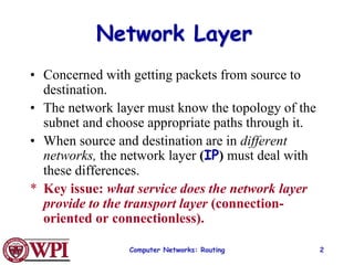
The document discusses routing in computer networks at the network layer. It covers routing algorithms like distance vector routing, link state routing, OSPF, and BGP. Distance vector routing uses hop counts as the metric and is prone to slow convergence. Link state routing floods link state information to all routers to compute shortest paths more quickly. OSPF and BGP are examples of link state and path vector routing protocols used between autonomous systems on the Internet.
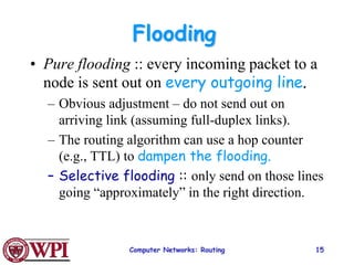
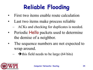
![Computer Networks: Routing 16
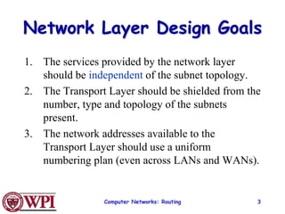
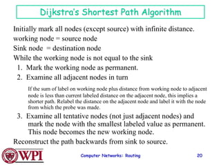
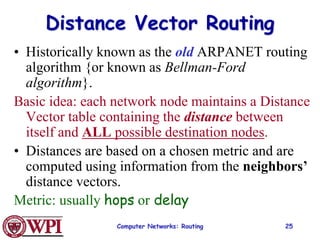
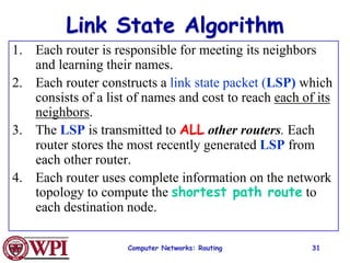
Shortest Path Routing
1. Bellman-Ford Algorithm [Distance Vector]
2. Dijkstra’s Algorithm [Link State]
What does it mean to be the shortest (or optimal)
route?
Choices:
a. Minimize the number of hops along the path.
b. Minimize mean packet delay.
c. Maximize the network throughput.](https://image.slidesharecdn.com/networklayer-220425140655/85/Network_Layer-ppt-16-320.jpg)
![Computer Networks: Routing 21
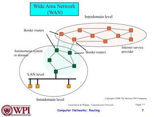
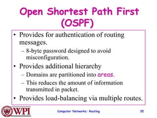
Internetwork Routing [Halsall]
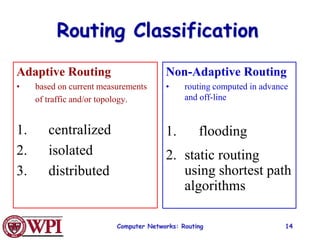
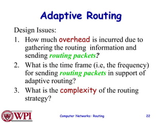
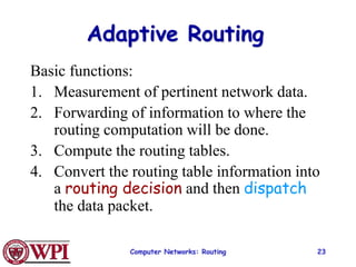
Adaptive Routing
Centralized Distributed
Intradomain routing Interdomain routing
Distance Vector routing Link State routing
[IGP] [EGP]
[BGP,IDRP]
[OSPF,IS-IS,PNNI]
[RIP]
[RCC]
Interior
Gateway Protocols
Exterior
Gateway Protocols
Isolated](https://image.slidesharecdn.com/networklayer-220425140655/85/Network_Layer-ppt-21-320.jpg)
![Computer Networks: Routing 27
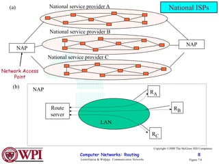
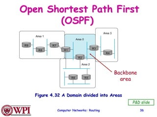
Distance Vector Algorithm
[Perlman]
1. A router transmits its distance vector to each of its
neighbors in a routing packet.
2. Each router receives and saves the most recently
received distance vector from each of its
neighbors.
3. A router recalculates its distance vector when:
a. It receives a distance vector from a neighbor containing
different information than before.
b. It discovers that a link to a neighbor has gone down (i.e., a
topology change).
The DV calculation is based on minimizing the cost
to each destination.](https://image.slidesharecdn.com/networklayer-220425140655/85/Network_Layer-ppt-27-320.jpg)
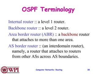
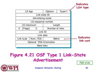
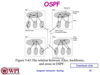
![Computer Networks: Routing 39
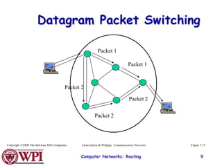
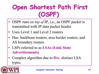
OSPF LSA Types
1. Router link advertisement [Hello message]
2. Network link advertisement
3. Network summary link advertisement
4. AS border router’s summary link
advertisement
5. AS external link advertisement](https://image.slidesharecdn.com/networklayer-220425140655/85/Network_Layer-ppt-39-320.jpg)
![Computer Networks: Routing 41
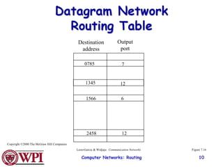
Area 0.0.0.1
Area 0.0.0.2
Area 0.0.0.3
R1
R2
R3
R4
R5
R6 R7
R8
N1
N2
N3
N4
N5
N6
N7
To another AS
Area 0.0.0.0
R = router
N = network
Figure 8.33
Copyright ©2000 The McGraw Hill Companies Leon-Garcia & Widjaja: Communication Networks
OSPF Areas
[AS Border router]
ABR](https://image.slidesharecdn.com/networklayer-220425140655/85/Network_Layer-ppt-41-320.jpg)


![Unit-3-Part-1 [Autosaved].ppt](https://cdn.slidesharecdn.com/ss_thumbnails/unit-3-part-1autosaved-230216062941-16596250-thumbnail.jpg?width=640&height=640&fit=bounds)