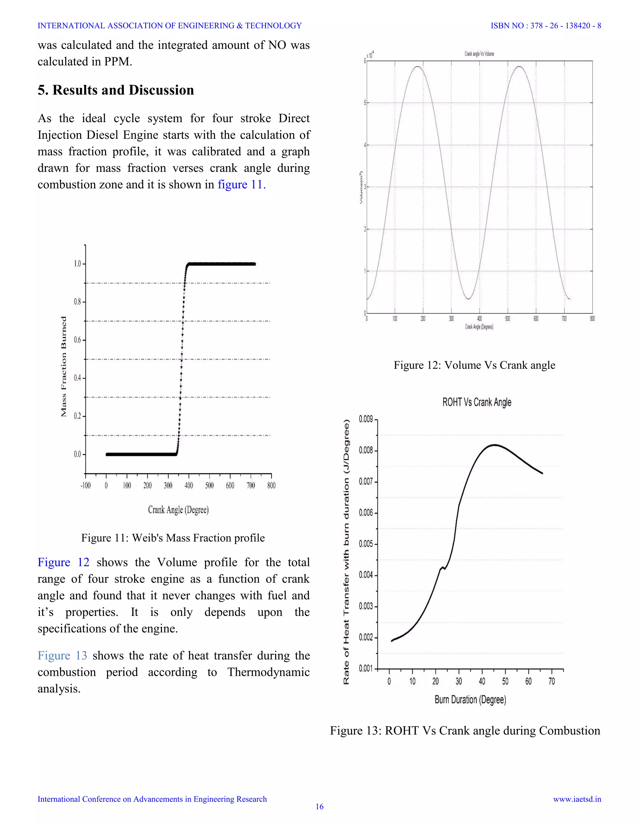
Iaetsd computer simulation of compression ignition engine through matlab

Computer Simulation of Compression Ignition Engine through
MATLAB
K. Hareesh1*, Rohith Teja. N2
, B. Konda Reddy3
1,
rgu.konankihareesh.1820@gmail.com, 2,
rohithteja.ps91221@gmail.com, 3,
bkondareddy.rkv@rgukt.in
1,2
Students in Bachelor of Technology, 3
Asst. Professor in Department of Mechanical Engineering.
1,2,3
Rajiv Gandhi University of Knowledge Technology, RK Valley, Andhra Pradesh – 516329.
Abstract:
In the present work, a computer simulation has been developed using MATLAB to determine the performance of
a four stroke Compression Ignition internal combustion (IC) engine. The modeling of this process begins with the
simulation of one cylinder of the four stroke IC engine which is assumed to have an ideal pressure-volume (p-V)
relationship allowing for computation of peak performance. The computer simulation is modeled for Ideal Cycle
System with encryption of thermodynamic laws of heat transfer and then it is also modeled for the prediction of
emissions.
The second phase of the model focuses on fuel cycle system where all the real factors are to be considered
for the prediction of performance parameters and emissions. Along with the thermodynamic model to compute
heat release some standard models like Woschni and Annand models are also used to predict the heat release.
Performance parameters computed include brake power and brake specific fuel consumption for an engine's entire
operating range.
Keywords: Computer simulation, IC engines, Ideal cycle system, Heat release models, Performance parameters,
Specific fuel consumption, MATLAB simulation.
1. Introduction
One of the major polluting contributors to our
environment today is the internal combustion engine,
either in the form of spark ignition (Otto) or Diesel
versions. In parallel to this serious environmental
threat, the main source of fuel for these engines, crude
oil, is being depleted at high rates, so that the
development of less polluting and more efficient
engines is today of extreme importance for engine
manufacturers. Also, to this end, the fact of the
increasing threat posed by the rivals of the internal
combustion engine, for smaller size engines, such as the
electric motors, the hybrid engines, the fuel cells and
the like corroborates the importance [1].
Experimental work aimed at fuel economy and low
pollutants emissions from Diesel and Otto engines
includes successive changes of each of the many
parameters involved, which is very demanding in
terms of money and time. Today, the development of
powerful digital computers leads to the obvious
alternative of simulation of the engine performance
by a mathematical model. In these models, the effects
of various design and operation changes can be
estimated in a fast and non-expensive way, provided
that the main mechanisms are recognized and
correctly modelled [2, 3].
The process of combustion in a Diesel engine is
inherently very complex due to its transient and
heterogeneous character, controlled mainly by turbulent
mixing of fuel and air in the fuel jets issuing from the
nozzle holes. High speed photography studies and in-
INTERNATIONAL ASSOCIATION OF ENGINEERING & TECHNOLOGY
International Conference on Advancements in Engineering Research
ISBN NO : 378 - 26 - 138420 - 8
www.iaetsd.in
5

cylinder sampling techniques have revealed some
interesting features of combustion [4]. The first
attempts to simulate the Diesel engine cycle substituted
the ‘‘internal combustion’’ by ‘‘external heat
addition’’. Apparent heat release rates were empirically
correlated to fuel injection rates and eventually used in
a thermodynamic cycle calculation to obtain the
cylinder pressure in a uniform mixture [5]. Models
based on droplet evaporation and combustion, while
still in a mono-zone mixture, can only partially take
into account the heterogeneous character of Diesel
combustion [4].
The need for accurate predictions of exhaust emissions
pollutants forced the researchers to attempt developing
two zone combustion models [1–4]. Eventually, some
multi-zone combustion models have appeared, carrying
the expected drawbacks of the first attempts, where the
detailed analysis of fuel-air distribution permits
calculation of the exhaust gas composition with
reasonable accuracy [3-6]. However, this happens under
the rising computing time cost when compared to lower
zones Diesel combustion models. At this point, it is
mentioned that multi-dimensional models have proved
useful in examining problems characterized by the need
for detailed spatial information and complex
interactions of many phenomena simultaneously [6, 7].
However, these are limited by the relative inadequacy
of sub-models for turbulence, combustion chemistry
and by computer size and cost of operation to crude
approximations to the real flow and combustion
problems.
Therefore, it is felt that a reasonable choice seems to be
a two zone model, which includes the effects of
changes in engine design and operation on the details of
the combustion process through a phenomenological
model where the geometric details are fairly well
approximated by detailed modelling of the various
mechanisms involved [1, 8]. This is going to have the
advantage of relative simplicity and very reasonable
computer time cost.
Thus, the object of the present work concerns a
comprehensive two zone model, applied to a direct
injection (DI) Diesel engine, similar in broad outline to
others, but with several differences that one must
expect from an independent research source. The model
contains upgraded jet mixing, heat transfer and
chemistry sub-models, using as simply as possible the
numerical analysis treatment of the governing
differential and algebraic equations, thus leading to
good solution convergence with reduced computer time
cost [9, 10].
Extending that work further, the present paper, after
exposing a rather short description of the model, as a
first step, verifies its validity by using data from a
vast experimental investigation. This data is taken at
the authors laboratory on a fully automated test bed,
four stroke, water cooled, standard ‘‘Hydra’’, direct
injection, high speed, Diesel engine. Plots of pressure,
temperatures in the two zones, nitric oxide (NO)
concentration, soot density, efficiency and other
interesting quantities are presented as a function of
crank angle, for various loads and injection timings,
providing insight into the physical mechanisms
governing the combustion and pollutants formation.
After gaining confidence in the predictive
capabilities of the model, the second step follows with
an extensive investigation of the sensitivity of the
model to variation of the constants used in the fuel
preparation and reaction sub-models, which are
proved critical to the model predictions. For this
purpose, the coincident experimental and predicted
points are used as baseline values around which
changes to these constants are effected. As a
feedback, this leads to a better understanding of the
physical mechanisms governed by these constants,
explaining the behavior of the combustion and
pollutants formation for various fuels and conditions
used, as reported in the literature. At the same time,
this analysis paves the way for the construction of a
reliable and relatively simple multi-zone model,
which incorporates in each zone (packet) the
philosophy of the present two zone model, while it
may also be useful for the construction of a
combustion model during transient engine operation
[8,11,12].
ISBN NO : 378 - 26 - 138420 - 8
www.iaetsd.in
6

2. Thermodynamic Analysis
Two-zone model views the entire combustion in to
burned zone and unburned zone as shown in the
Figure 1.
fat mmm 
  itib mmm 
After amount of mass fraction burned inside the
combustion chamber was found out, the next
important parameter to find out is instantaneous
Volume of the cylinder. This volume can be obtained
by the equation in relation with the crank angle as:
Figure 1: Two Zone Combustion Model
However, the two-zone model recognizes a burned
and unburned zone, thus predicting heat transfer and
emissions more accurately. The construction of two
zone model begins with weibe function to identify
burned and unburned regions.
 
 
)908.6exp(1
1





 

b
d
i



The mass fraction profile follows the ‘S’. So, that’s
why it is called as S-function. The burn profile is
engine-specific.
So, from the mass fraction profile the total amount of
mass burned inside the chamber can be find out as:
int
intint
TR
VP
m
g
a



fm mass of fuel
     
 2/1221
2
sincos1
4








 
r
D
VclV
The peculiarity of this process among all other
processes of combustion analysis is, here the total
combustion range is divided into six regions such as
suction, Compression, Combustion, expansion,
constant volume heat rejection and exhaust. All the
processes in the above listed will follow the ideal
relations show in the below Figure 2.
Figure 2: Diesel Cycle
But, the prediction of performance parameters in
combustion zone is bit complicated and doesn’t
follow the ideal relations. Generally in the
combustion region, Volume and Temperature does
not remains constant which leads to the increasing of
Burned
zone
Unburned
zone
ISBN NO : 378 - 26 - 138420 - 8
www.iaetsd.in
7

Figure 4(b): PV Diagram
Figure 4(a): Pressure Vs Theta
pressure as the combustion proceeds. Inorder to find
the pressure the temperature has to be obtained by
using heat equations shown below:
    )( TTCmLHVmQ newpubin  
From the above relation new temperature can be
obtained as
   
pu
b
new
Cm
LHVm
TT





Temperature increases rapidly during the combustion
and then decreases due to heat convection by cooling
water. The temperature in the total cycle changes as
show in below Figure 3.
Figure 3: Variation of Temperature in combustion zone
Now the new pressure can be obtained as
 
 
 


V
TRm
P
newgt
new


In actual combustion process unlike the idea case the
pressure doesn’t remain constant at heat addition
process, rather it reaches a maximum value at
maximum heat addition point and then decreases.
This is because that there was no assumption that the
pressure remains constant in the region of
combustion. The following Figure 4a, 4b justify the
above information and also gives an idea of PV-
Diagram:
ISBN NO : 378 - 26 - 138420 - 8
www.iaetsd.in
8

Rated Powers and Efficiencies
This section starts with the calculation of total work
done in the cycle from where mean effective pressure
can be calculated which is equal to the Indicated
mean effective pressure when the friction is neglected
[5]. The work output can be obtained from
 
11
112max4433
23max







VPVPVPVP
VVPW
Then the Indicated power is







60
n
WI p (KW), where n = N/2 for four stroke
engine
From the pI mean effective pressure was obtained
from,
LAnK
I
imep
p

60000
(Pa)
Friction mean effective pressure for direct injection
diesel engine is given [6] as
2
4.0
1000
48 pU
RPM
Cfmep 






Where C is constant which is equal to 75 Kpa and Up
is the mean piston speed.
Then friction power is,
60000
LAnKfmep
Fp


Now, the brake Power and brake mean effective
pressure are obtained from the following relations
ppp FIB 
LAnK
B
bmep
p

60000
Once the all rates powers were obtained calculation of
their efficiencies becomes easy. The brake thermal
efficiency is obtained [4] as
CVMFVL
B
BTH
p


Where MFVLis the fuel in terms of Kg/s
Then the brake specific fuel consumption is
determined as
pB
MFVL
BSFC
3600

The brake specific fuel consumption varies with the
load, fuel and engine model. It is high at full load
condition where maximum power output is generated
in the form of brake power [4].
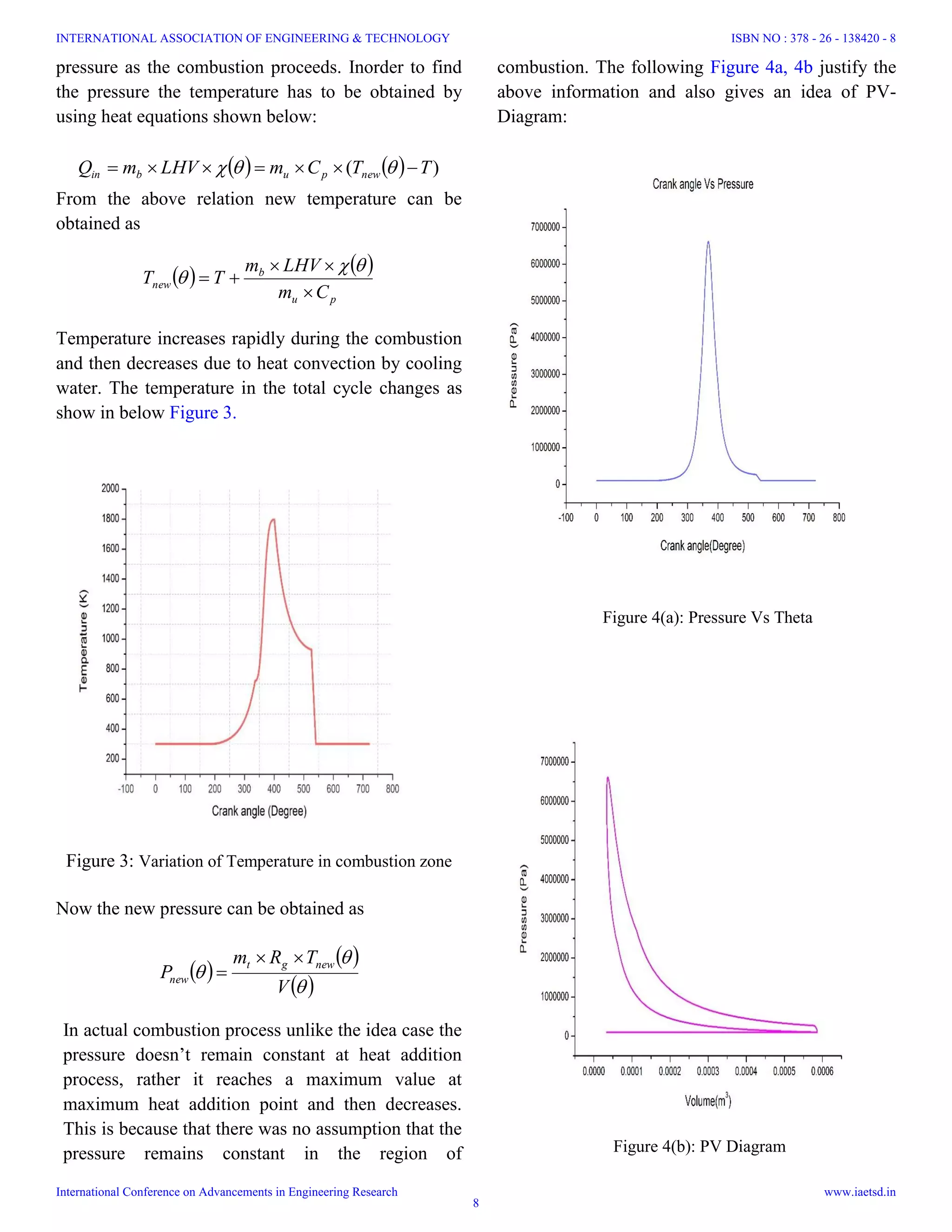
Heat Release Models
This section starts with the first law of
thermodynamics for the four stroke engine energy
balance [3] is
WQU 
Where Q the total energy is transferred into the
system, W is the work transferred out of the system,
and U is the change in internal energy within the
system. In differentiating equation the above equation
with respect to d







 d
dT
mC
d
dW
d
dQ
d
dU
v
Where vC is the specific heat of the combustion
chamber gas. Upon dividing the specific heat by the
universal gas constant [9],
1
1




vp
vv
CC
C
R
C
Where  is the specific heat ratio.
The above equations can be used to describe the
formation of work and the net heat input:







 d
dV
P
d
dW
 d
dQ
d
dQ
d
dQ lossinn

Which can be expanded as,


 d
dQ
d
d
LHVm
d
dQ loss
f
n







ISBN NO : 378 - 26 - 138420 - 8
www.iaetsd.in
9

Figure 5: Rate of change of convective heat transfer
coefficient with crank angle
If we further implements the heat model to get net
heat with respect to crank angle [3], the equation
becomes:


 d
dP
V
d
dV
P
d
dQn
1
1
1 



However, it is also necessary to continue discussion
to get more accuracy for more complex heat release
models. Lastly the change in pressure [6] is defined
by:




 d
dV
V
P
d
dQ
d
dQ
Vd
dP lossin









1
The rate of heat loss can be expressed as
       









1
w
loss
TTAh
d
dQ
This can be modelled by two models namely
woschni’s heat transfer model and Annand’s heat
transfer model.
Woschni’s Heat Release Model
Woschni’s method is a set of empirical equations that
predicts the heat transfer coefficient between in-
cylinder gasses and walls [5]. The convective losses
between in-cylinder gasses and walls can be predicted
using Newton’s law of cooling:
     














100100
76.5
1
44
w
w
ht TT
TTAh
d
dQ 




 h is the instantaneous heat transfer coefficient,
 A is the instantaneous heat transfer area, T is the
instantaneous bulk gas temperature, and wT is the
cylinder wall temperature. With the heat loss
modelled angularly, the convective heat transfer
coefficient is now defined as:
  8.055.08.02.0
26.3 wTPDh 

Where that w denotes the woschni’s factor which
also changes with the crank angle and it is expressed
[11] [12] [4] as,
    m
rr
r
p PP
VP
TV
CUw   
128.2
Where 1C the constant is varies with the process. For
combustion process 1C =0.00324, pU is mean piston
speed, V is the instantaneous volume, rT is the
reference temperature, rP is the reference pressure, rV
is the reference volume,  P instantaneous pressure
at the combustion period and mP is the motored
cylinder pressure.
In compression and expansion processes, Watson and
Janota [6] suggested modelling the motored cylinder
pressure as a polytrophic process:









V
V
PP r
rm
With all of these variables previously expressed, the
convective heat transfer coefficient and corresponding
heat loss could then be calculated.
ISBN NO : 378 - 26 - 138420 - 8
www.iaetsd.in
10

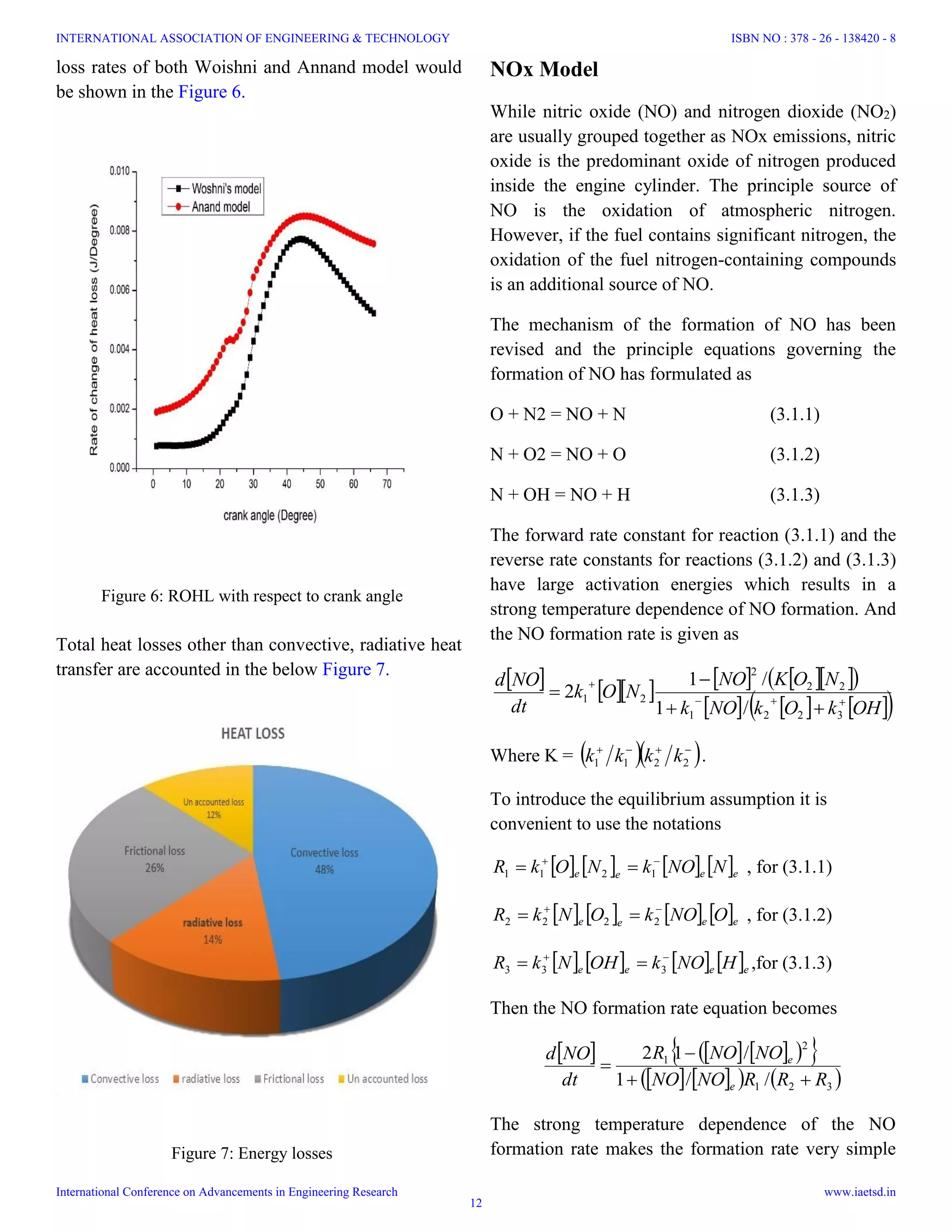
The change in convective heat transfer coefficient
with the crank angle during combustion according
woschni’s has represented in the Figure 5.
Annand’s Heat Release Model
Annand’s and Woschni’s heat transfer models
differed in the fact that Annand’s approach separated
the convective and radiation terms. Annand’s method
solved for the heat transfer coefficient by assuming
pipe-like fluid dynamics, and using the in-cylinder
density, and Reynolds and Nusselt numbers as
functions of time.
Using Annand’s method, Newton’s law of cooling
can be broken into convective and radiation terms [3]
as follows:
        








 
1
wrc TTAhh
d
dQ
Where  ch is the convective heat transfer
coefficient and  rh is the radiation heat transfer
coefficient. The convective heat transfer coefficient
can be extracted from the relationship between the
Nusselt number and fluid properties [7] as
D
Nuk
h
gas
c 
Where gask is the gas thermal conductivity, Nu is the
Nusselt number, and Dis the cylinder bore. With an
iterative solver, the thermal conductivity of the
cylinder gas can be modelled using a polynomial
curve-fitting of experimental data. Heywood [2]
suggests using the curve fitted equation:
2853
102491.1103814.7101944.6  TTkgas


, units are 





Km
W
*
The Nusselt number can be described relative to the
Reynolds number and the type of engine:
7.0
ReaNu 
Where a is a constant having a value of 0.26 for a
two-stroke engine and 0.49 for a four stroke engine
[2], and is the instantaneous Reynolds number. The
Reynolds number is expressed as:
gas
pgas DU


Re
Where gas is the instantaneous cylinder gas density,
pU is the mean piston velocity, and gas is the
instantaneous gas viscosity. Since the model assumes
ideal gas behavior, the cylinder gas density can be
found by rearranging the ideal gas law:
TR
P
gas
gas 
Where gasR is the fluid-specific gas constant, and an
assumed value of 287[
KgK
J
] was used for this
variable.
As with the thermal conductivity, the cylinder gas
viscosity was modelled using empirical equations.
According to Heywood [2], the cylinder gas viscosity
can be expressed as:
212
104793.7
8
101547.4
6
.10457.7
*
 TT
sm
kg
gas











Although the radiative heat transfer coefficient is
small [2], it was decided that radiation should be
included in considering overall heat losses in the
model. The radiative heat transfer coefficient is
defined as [5]:















 
w
w
r
TT
TT
Km
w
h


4
9
2
1025.4
*
Where the instantaneous cylinder temperature and
wall temperature must be provided in units of [K].
With known pressure and temperature traces from the
calculations, Annand’s method could then be used to
calculate heat losses. A comparison of predicted heat
ISBN NO : 378 - 26 - 138420 - 8
www.iaetsd.in
11

Figure 7: Energy losses
Figure 6: ROHL with respect to crank angle
loss rates of both Woishni and Annand model would
be shown in the Figure 6.
Total heat losses other than convective, radiative heat
transfer are accounted in the below Figure 7.
NOx Model
While nitric oxide (NO) and nitrogen dioxide (NO2)
are usually grouped together as NOx emissions, nitric
oxide is the predominant oxide of nitrogen produced
inside the engine cylinder. The principle source of
NO is the oxidation of atmospheric nitrogen.
However, if the fuel contains significant nitrogen, the
oxidation of the fuel nitrogen-containing compounds
is an additional source of NO.
The mechanism of the formation of NO has been
revised and the principle equations governing the
formation of NO has formulated as
O + N2 = NO + N (3.1.1)
N + O2 = NO + O (3.1.2)
N + OH = NO + H (3.1.3)
The forward rate constant for reaction (3.1.1) and the
reverse rate constants for reactions (3.1.2) and (3.1.3)
have large activation energies which results in a
strong temperature dependence of NO formation. And
the NO formation rate is given as
          
      OHkOkNOk
NOKNO
NOk
dt
NOd





3221
22
2
21
/1
/1
2
Where K =   
2211 kkkk .
To introduce the equilibrium assumption it is
convenient to use the notations
       eeee NNOkNOkR 
 1211 , for (3.1.1)
       eeee ONOkONkR 
 2222 , for (3.1.2)
       eeee HNOkOHNkR 
 333 ,for (3.1.3)
Then the NO formation rate equation becomes
       
      321
2
1
//1
/12
RRRNONO
NONOR
dt
NOd
e
e



The strong temperature dependence of the NO
formation rate makes the formation rate very simple
ISBN NO : 378 - 26 - 138420 - 8
www.iaetsd.in
12

Crevices
48%
oil layers
22%
valves
5%
others
25%
HC EMISSION
CONTRIBUTIONS
Figure 9: % of factors contributing to HC emissions
Figure 8: NOx emissions with respect to Temperature.
and depends on the equilibrium concentration of
Oxygen and Nitrogen and it is given as
     ee NO
T
T
dt
NOd
2
2/1
2
2
1
16
69090
exp
106





 

The strong dependence of
 
dt
NOd
on temperature in
the exponential term is evident. High temperatures
and high oxygen concentrations result in high NO
formation rates. The characteristic time for the NO
formation process is
 
2/1
16
/58300exp108
P
TT
NO



By multiplying this time with NOx formation rate we
can get the NOx in to PPM as
NOx (PPM) =
 












3600
1000
106
NO
dt
NOd

The change in NOx emission in PPM with respect to
temperature is shown in the Figure 8.
HC Model
Hydrocarbons, or more appropriately organic
emissions, are the consequence of incomplete
combustion of the hydrocarbon fuel. The level of
unburned hydrocarbons (HC) in the exhaust gases is
generally specified in terms of the total hydrocarbons
concentration expressed in parts per million carbon
atoms.
A reasonable fit to the experimental data on unburned
HC burn up is the rate expression [9] as
  2
15
2
18735
exp107.6 










 

RT
P
xx
Tdt
HCd
OHC
Where 2
, OHC xx are the mole fraction of HC and mole
fraction of Oxygen respectively.
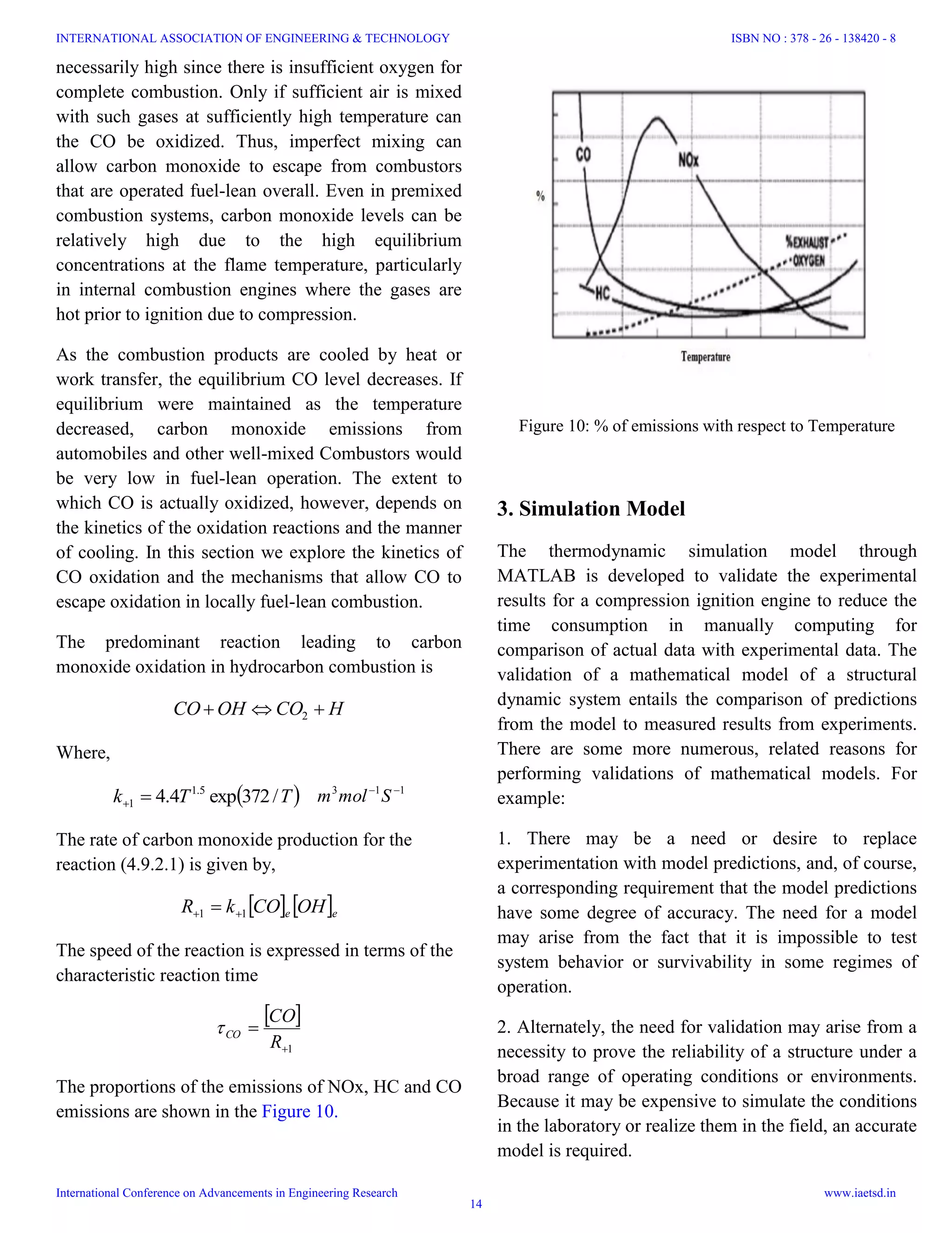
The main contribution of unburned Hydro Carbons
are depicted in the Figure 9.
CO Emissions
Carbon monoxide is an intermediate species in the
oxidation of hydrocarbon fuels to CO2 and H2O. In
fuel-rich regions of a flame, the CO levels are
ISBN NO : 378 - 26 - 138420 - 8
www.iaetsd.in
13

necessarily high since there is insufficient oxygen for
complete combustion. Only if sufficient air is mixed
with such gases at sufficiently high temperature can
the CO be oxidized. Thus, imperfect mixing can
allow carbon monoxide to escape from combustors
that are operated fuel-lean overall. Even in premixed
combustion systems, carbon monoxide levels can be
relatively high due to the high equilibrium
concentrations at the flame temperature, particularly
in internal combustion engines where the gases are
hot prior to ignition due to compression.
As the combustion products are cooled by heat or
work transfer, the equilibrium CO level decreases. If
equilibrium were maintained as the temperature
decreased, carbon monoxide emissions from
automobiles and other well-mixed Combustors would
be very low in fuel-lean operation. The extent to
which CO is actually oxidized, however, depends on
the kinetics of the oxidation reactions and the manner
of cooling. In this section we explore the kinetics of
CO oxidation and the mechanisms that allow CO to
escape oxidation in locally fuel-lean combustion.
The predominant reaction leading to carbon
monoxide oxidation in hydrocarbon combustion is
HCOOHCO  2
Where,
 TTk /372exp4.4 5.1
1 
113 
Smolm
The rate of carbon monoxide production for the
reaction (4.9.2.1) is given by,
   ee OHCOkR 11  
The speed of the reaction is expressed in terms of the
characteristic reaction time
 
1

R
CO
CO
The proportions of the emissions of NOx, HC and CO
emissions are shown in the Figure 10.
3. Simulation Model
The thermodynamic simulation model through
MATLAB is developed to validate the experimental
results for a compression ignition engine to reduce the
time consumption in manually computing for
comparison of actual data with experimental data. The
validation of a mathematical model of a structural
dynamic system entails the comparison of predictions
from the model to measured results from experiments.
There are some more numerous, related reasons for
performing validations of mathematical models. For
example:
1. There may be a need or desire to replace
experimentation with model predictions, and, of course,
a corresponding requirement that the model predictions
have some degree of accuracy. The need for a model
may arise from the fact that it is impossible to test
system behavior or survivability in some regimes of
operation.
2. Alternately, the need for validation may arise from a
necessity to prove the reliability of a structure under a
broad range of operating conditions or environments.
Because it may be expensive to simulate the conditions
in the laboratory or realize them in the field, an accurate
model is required.
Figure 10: % of emissions with respect to Temperature
ISBN NO : 378 - 26 - 138420 - 8
www.iaetsd.in
14

3. Another reason for model validation is that a system
may be undergoing changes in design that require
analyses to assure that the design modifications yield
acceptable system behaviour. A validated model can be
used to assess the system behaviour. In all these
situations it is useful to confirm analysts’ abilities to
produce accurate models.
In this work, the task of developing the MATLAB
simulation model for compression ignition engine is for
testing different fuels at different conditions to select
the best to have high efficiency and less emissions.
4. MATLAB Script Procedure
In selecting a computer program to execute the
demands of a two-zone model, Matrix Laboratory
(MATLAB) was considered. It was considered as
because of its ease of simulation and speed of
validation. With keeping all constraints in mind total
script was developed in MATLAB for the future use.
The bulk of MATLAB code was set up through the use
of script and the total script is divided in to some sub
sections.the purpose of these sub-sections and the
organization of the MATLAB model will be elucidated
in subsequent sections.
4.1 Engine Geometry and Atmospheric inputs
The MATLAB script began with known engine inputs.
The bore, stroke, connecting rod length, number of
cylinders, compression ratio, and operating
characteristics has to mentioned to the program as
inputs for the validation of an experimental details.
Based on the inputs script would calculate the area of
the cylinder, clearance volume of the cylinder and
surface area of the piston head. And the atmospheric
conditions were chosen like, the initial inlet
Temperature 300K (room temperature) and pressure as
1 atm.
4.2 Pre-allocation of Arrays
Through experimentation, it was found that pre-
allocating arrays and matrices drastically improved
the efficiency of the program. This prevented
MATLAB from having to re-size arrays or matrices
between iterations, thus decreasing the overall
computation time. Pre-allocated arrays and matrices
were also used as a means of setting appropriate
properties for the recursion of the program to
compare between the graphs of multiple fuel tests.
4.3 Fuel inputs
Fuel inputs such as mass of the fuel, Calorific value,
Lower Heat Values and air-fuel ratio were taken as
per the experiment model of the engine.
4.4 Instantaneous Engine and Fluid Properties
In order to that the main program has divided in to
two sub loops where in the first loop with a
specified index (i=0:720) calculated instantaneous
engine properties discussed in the above section. In
addition to the properties of instantaneous
properties like volume, pressure and temperature it
has also scripted for to calculate work done during
the total range of the cycle, Indicated power,
friction power, brake power, correction factor for
the calculation of brake power and brake specific
fuel function.
The second loop with specified index in the range
of combustion, MATLAB script has statements to
cope up with heat release and heat loss model in
Woschni and Annand model.
4.5 Plot statements
Each plot was sized based on the minimum and
maximum variable values, and each plot was given
a title appropriate to the variable being plotted.
MATLAB script was so developed to have a plots
between all the performance parameters as a
function of crank angle, PV diagrams and for the
relation between pressure and temperature. Plots
were modelled for mass-fraction, heat release and
heat loss as a function of crank angle.
4.6 Emission Predictions
The NO prediction model was included in the
MATLAB script, predicted the quantitative fraction
of NO particles. The residence time for NO formation
ISBN NO : 378 - 26 - 138420 - 8
www.iaetsd.in
15

was calculated and the integrated amount of NO was
calculated in PPM.
5. Results and Discussion
As the ideal cycle system for four stroke Direct
Injection Diesel Engine starts with the calculation of
mass fraction profile, it was calibrated and a graph
drawn for mass fraction verses crank angle during
combustion zone and it is shown in figure 11.
Figure 12 shows the Volume profile for the total
range of four stroke engine as a function of crank
angle and found that it never changes with fuel and
it’s properties. It is only depends upon the
specifications of the engine.
Figure 13 shows the rate of heat transfer during the
combustion period according to Thermodynamic
analysis.
Figure 13: ROHT Vs Crank angle during Combustion
Figure 11: Weib's Mass Fraction profile
Figure 12: Volume Vs Crank angle
ISBN NO : 378 - 26 - 138420 - 8
www.iaetsd.in
16

Figure 14: Comparison of Heat transfer Coefficients of
both Woschni's and Annand Heat Release Models
Figure 14 show the difference between the heat
transfer coefficient for both Woschni’s and Annand
heat release models and found they follow same trend
as they follow for standard cycles systems.
Using the burned-zone temperature, sub-functions
were created to calculate NOx and HC emissions and
graphs were generated as shown in Figure 10.
Conclusion
It was found that the model could be used in
simulating any diesel engine. This could save an
enormous amount of time in tuning an engine,
especially when little is known about the engine. With
an air-fuel ratio and volumetric efficiency map,
Injection-timing could be optimized, thus minimizing
wear-and-tear on the engine and dynamometer
equipment. Much research could be directed towards
refining the model and using it for the improvement
of engine performance and reducing the NOx
emissions by testing different fuels.
References
1. C.D. Rakopoulos, E.G. Giakoumis and D.C.
Kyritsis - “Validation and sensitivity analysis of a
two zone Diesel engine model for combustion and
emissions prediction”, Energy Conversion and
Management 45 (2004).
2. Jeremy L. Cuddihy - University of Idaho, “A
User-Friendly, Two-Zone Heat Release Model for
Predicting Spark-Ignition Engine Performance
and Emissions”, May 2014.
3. “Computer Simulation of Compression Engine”
by V. Ganesan –1st
edition, 2000.
4. J. Heywood, Internal Combustion Engine
Fundamentals. Tata Mcgraw Hill Education, 2011.
5. V. Ganesan, Internal Combustion Engines, 6th
edition, Tata Mcgraw Hill Education, 2002.
6. Zehra Sahin and Orhan Durgun - “Multi-zone
combustion modeling for the prediction of diesel
engine cycles and engine performance
parameters”, Applied Thermal Engineering 28
(2008).
7. G. P. Blair, Design and Simulation of Four Stroke
Engines [R-186]. Society of Automotive
Engineers Inc, 1999.
8. C.D. Rakopoulos, K.A. Antonopoulos and D.T.
Hountalas -“Multi-zone modeling of combustion
and emissions formation in DI diesel engine
operating on ethanol–diesel fuel blends”, Energy
Conversion and Management 49 (2008) 625–643.
9. Hsing-Pang Liu, Shannon Strank, MikeWerst,
Robert Hebner and Jude Osara - “COMBUSTION
EMISSIONSMODELING AND TESTING OF
CONVENTIONAL DIESEL FUEL”, Proceedings
of the ASME 2010, 4th International Conference
on Energy Sustainability (May 17-22, 2010).
10. A. Sakhrieh, E. Abu-Nada, I. Al-Hinti, A. Al-
Ghandoor and B. Akash - “Computational
thermodynamic analysis of compression ignition
engine”, International Communications in Heat
and Mass Transfer 37 (2010) 299–303 .
11. D. Descieux, M. Feidt - “One zone thermodynamic
model simulation of an ignition compression
engine”, Applied Thermal Engineering 27 (2007)
1457–1466.
12. Mike Saris, Nicholas Phillips - Computer
Simulated Engine Performance, 2003.
ISBN NO : 378 - 26 - 138420 - 8
www.iaetsd.in
17

Iaetsd computer simulation of compression ignition engine through matlab

More Related Content

What's hot

Viewers also liked

Similar to Iaetsd computer simulation of compression ignition engine through matlab

More from Iaetsd Iaetsd

Recently uploaded

Iaetsd computer simulation of compression ignition engine through matlab