Download to read offline


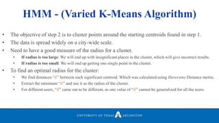
![• Our variation of the K-Means algorithm was influenced by [1] and [2].
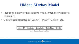
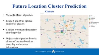
• Mainly focused on “where the user is instead of how the user got there”.
• Find the locations where a user spent most of their time.
• Targeted our algorithm to find the time elapsed between two consecutive
points.
• Identified the points which have more than “𝜏” between them and their
corresponding previous point.
• Another challenge was to find a significant value of “𝜏”.
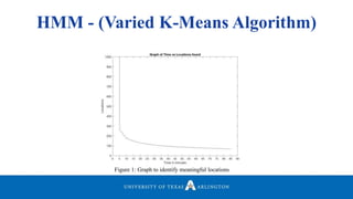
• Plotted a graph of Graph to Identify Meaningful Locations.
HMM - (Varied K-Means Algorithm)](https://image.slidesharecdn.com/defenseppt05292018-180611183402/85/Hyperoptimized-Machine-Learning-and-Deep-Learning-Methods-For-Geospatial-and-Temporal-Function-Estimation-11-320.jpg)
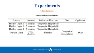
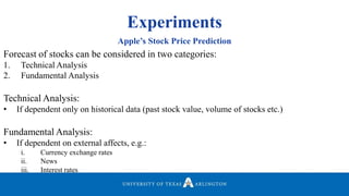
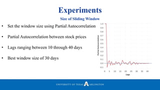
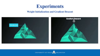
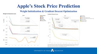
![Experiments
Weight Initialization and Gradient Descent
• 𝑍 = 𝑤1 𝑥1+ 𝑤2 𝑥2 + ⋯ + 𝑤 𝑛 𝑥 𝑛
• Good rule of thumb:
• Var(𝑊𝑖) =
1
𝑛
• Set variance of weights equal to
1/number of features in the dataset
• Lecun_Uniform: Named after its creator
Yann LeCun
• Lecun_uni: Draws samples from
uniform distribution within [-lim, lim]
• lim = 𝑠𝑞𝑟𝑡(
3
𝑓𝑎𝑛𝑖𝑛
)
• He_normal: Named after its creator
Kaiming He
• StdDev(𝑊𝑖) = 𝑠𝑞𝑟𝑡(
2
𝑓𝑎𝑛𝑖𝑛
)](https://image.slidesharecdn.com/defenseppt05292018-180611183402/85/Hyperoptimized-Machine-Learning-and-Deep-Learning-Methods-For-Geospatial-and-Temporal-Function-Estimation-68-320.jpg)
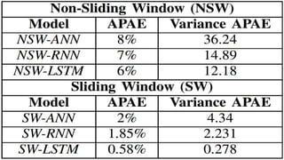

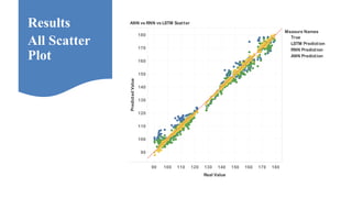


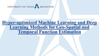
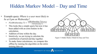
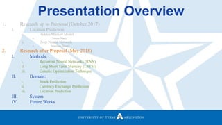
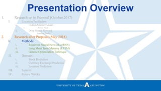
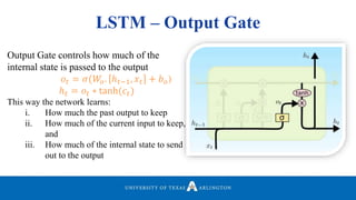
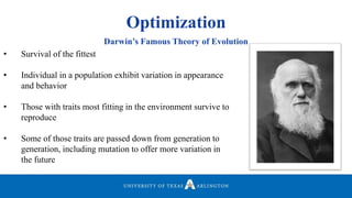
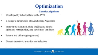
Neelabh Pant successfully defended his PhD thesis titled "Hyper-optimized Machine Learning and Deep Learning Methods for Geo-Spatial and Temporal Function Estimation" at the University of Texas at Arlington. His research focused on developing recurrent neural networks, long short-term memory models, and genetic optimization techniques to predict locations, stock prices, and currency exchanges based on spatio-temporal data. Pant's dissertation committee included Dr. Ramez Elmasri as his advisor along with four other professors who evaluated his work.