Download to read offline
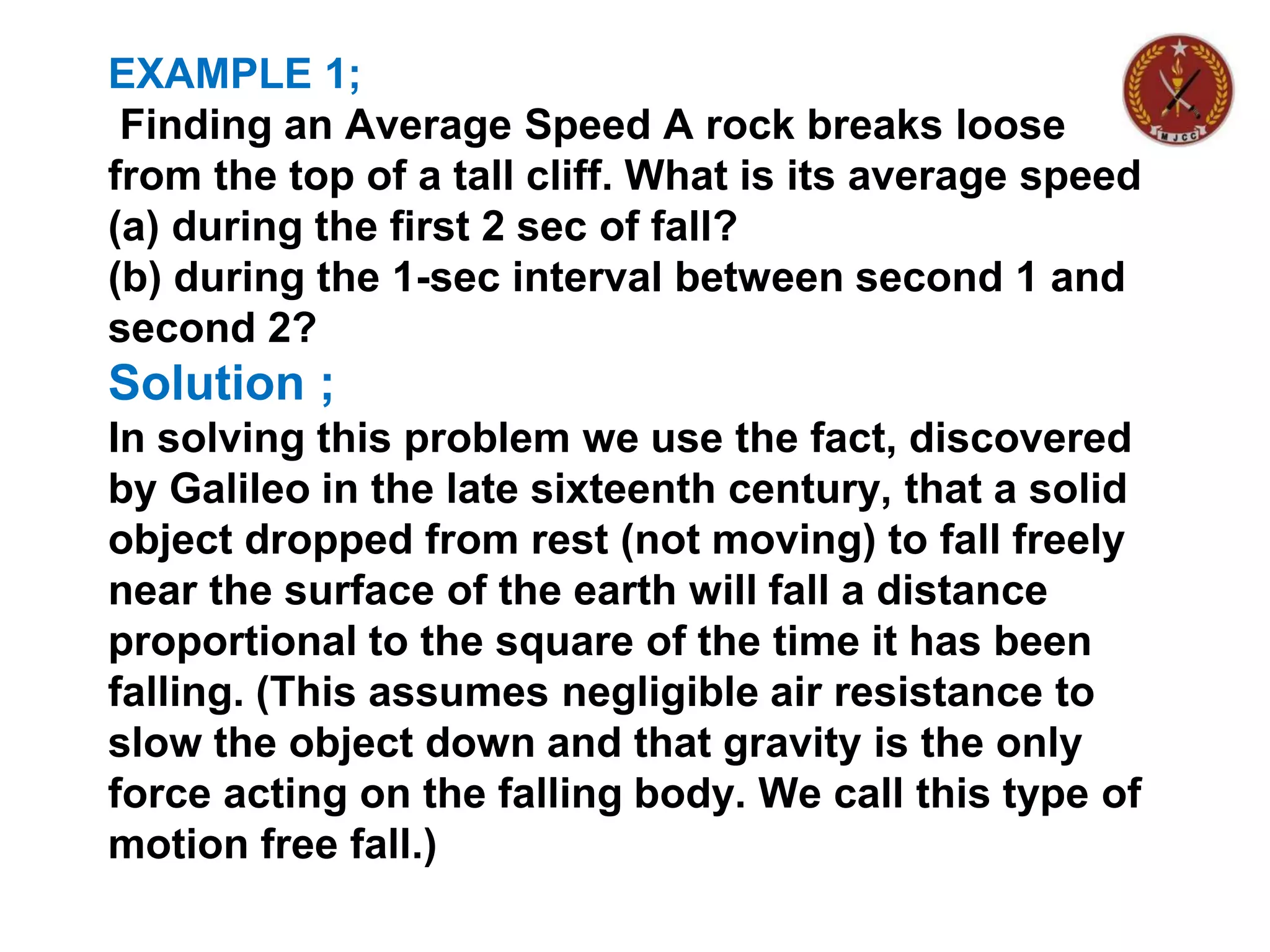
![EXAMPLE 2; Finding an Instantaneous Speed
The next example examines what happens when we look at
the average speed of a falling object over shorter and
shorter time intervals
Find the speed of the falling rock at t=1sec and t=2 sec.
Solution ; We can calculate the average speed of the rock
over a time interval [t0 t0+h] having length ∆t=h as
eq(1).
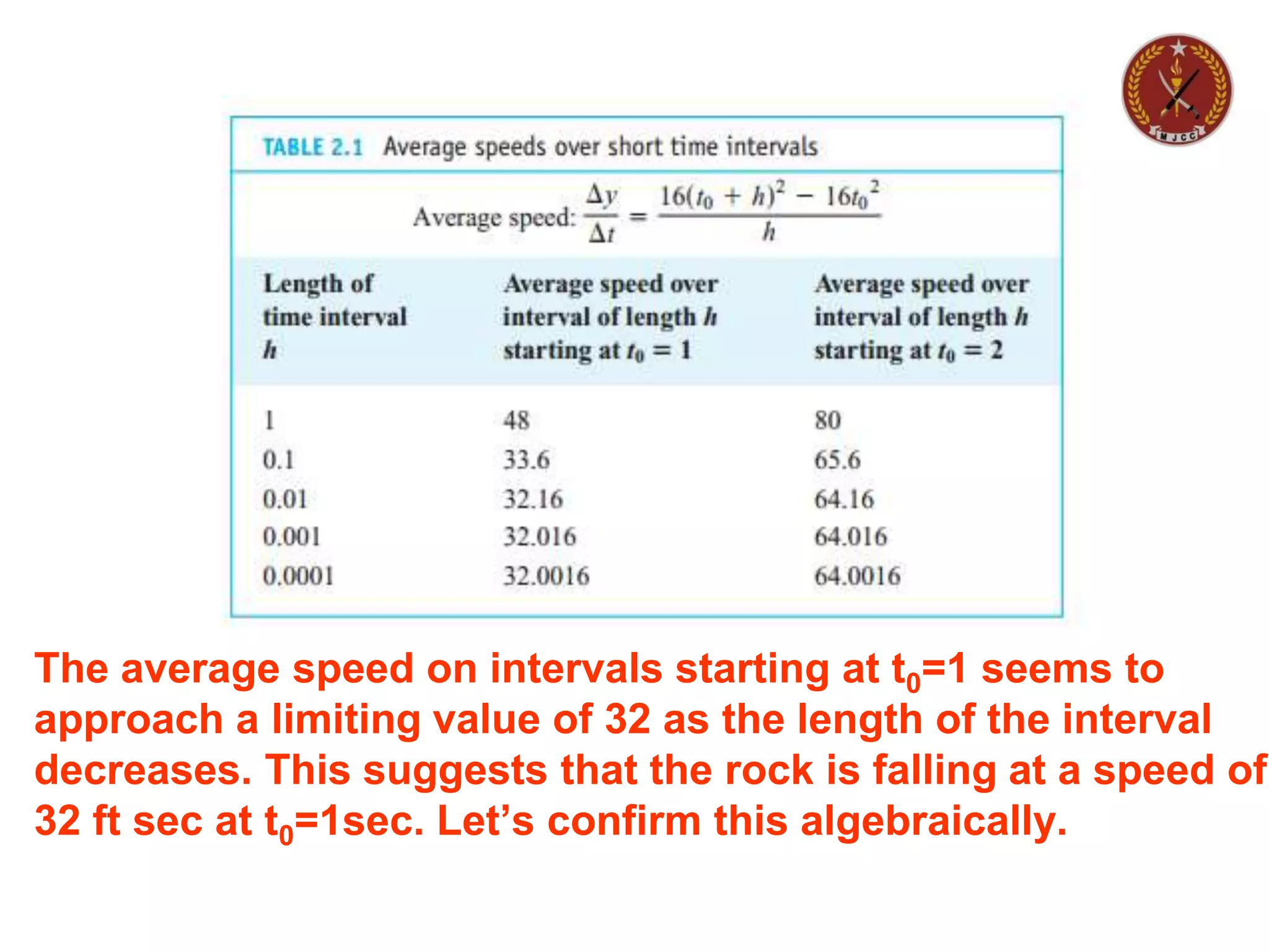
We cannot use this formula to calculate the “instantaneous” speed
at t0 by substituting h=0 because we cannot divide by zero. But we
can use it to calculate average speeds over increasingly short time
intervals starting at t0=1 &t0=2 and When we do so, we see a pattern
inTable](https://image.slidesharecdn.com/hsscii-introductionoflimits-210810070258/75/Hssc-ii-introduction-of-limits-9-2048.jpg)
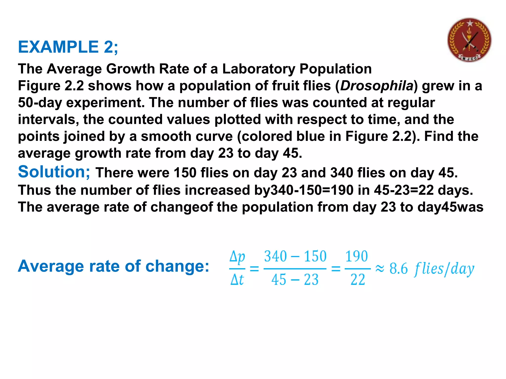
![Average Rates of Change and Secant Lines
Given an arbitrary function y=f(x). we calculate the average
rate of change of y with
respect to x over the interval [x1 x2], by dividing the change in
the value of y, ∆y=f(x2)-f(x1).by the length
∆x=x2-x1=h of the interval over which the
change occurs.](https://image.slidesharecdn.com/hsscii-introductionoflimits-210810070258/75/Hssc-ii-introduction-of-limits-12-2048.jpg)
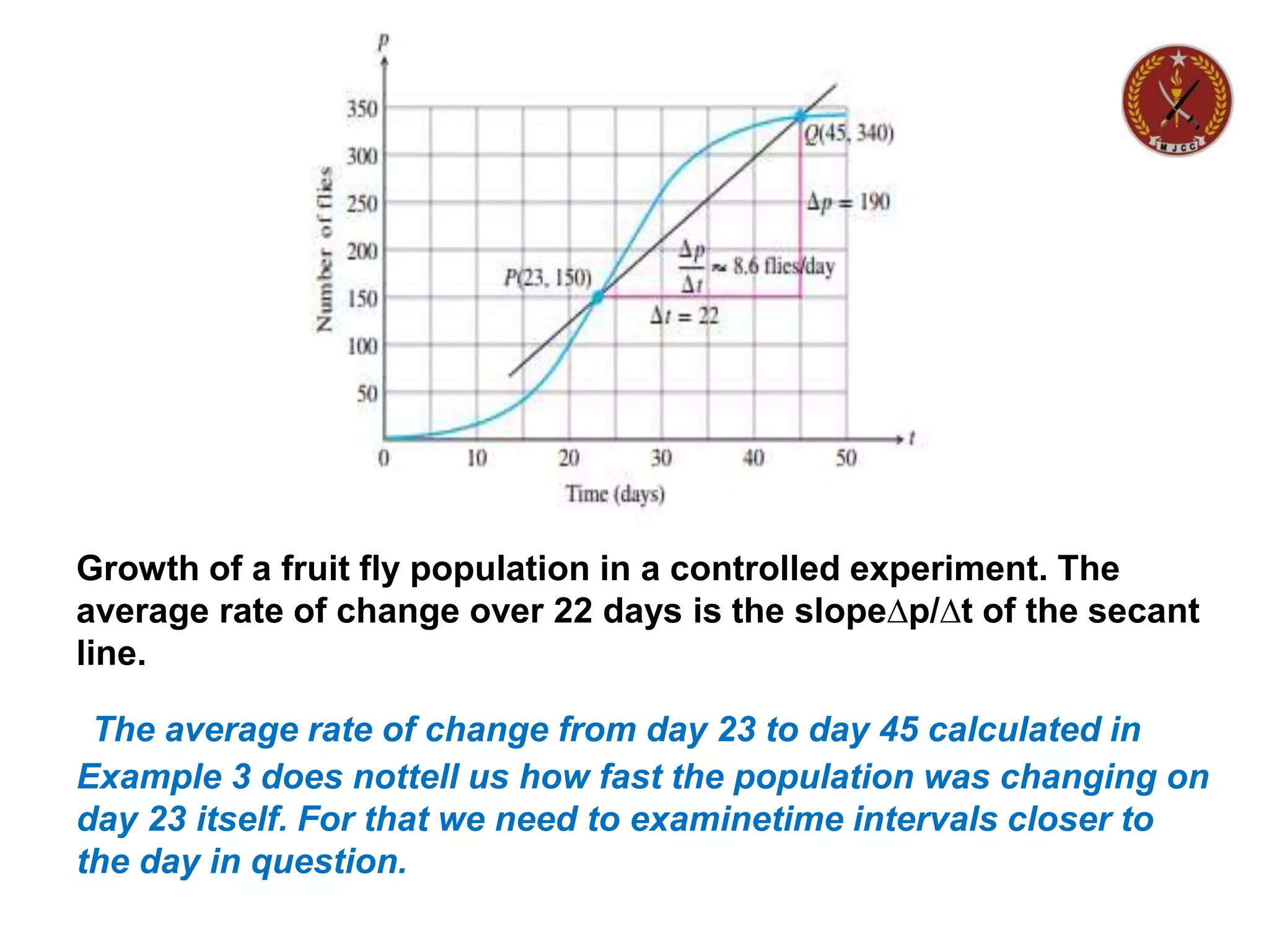
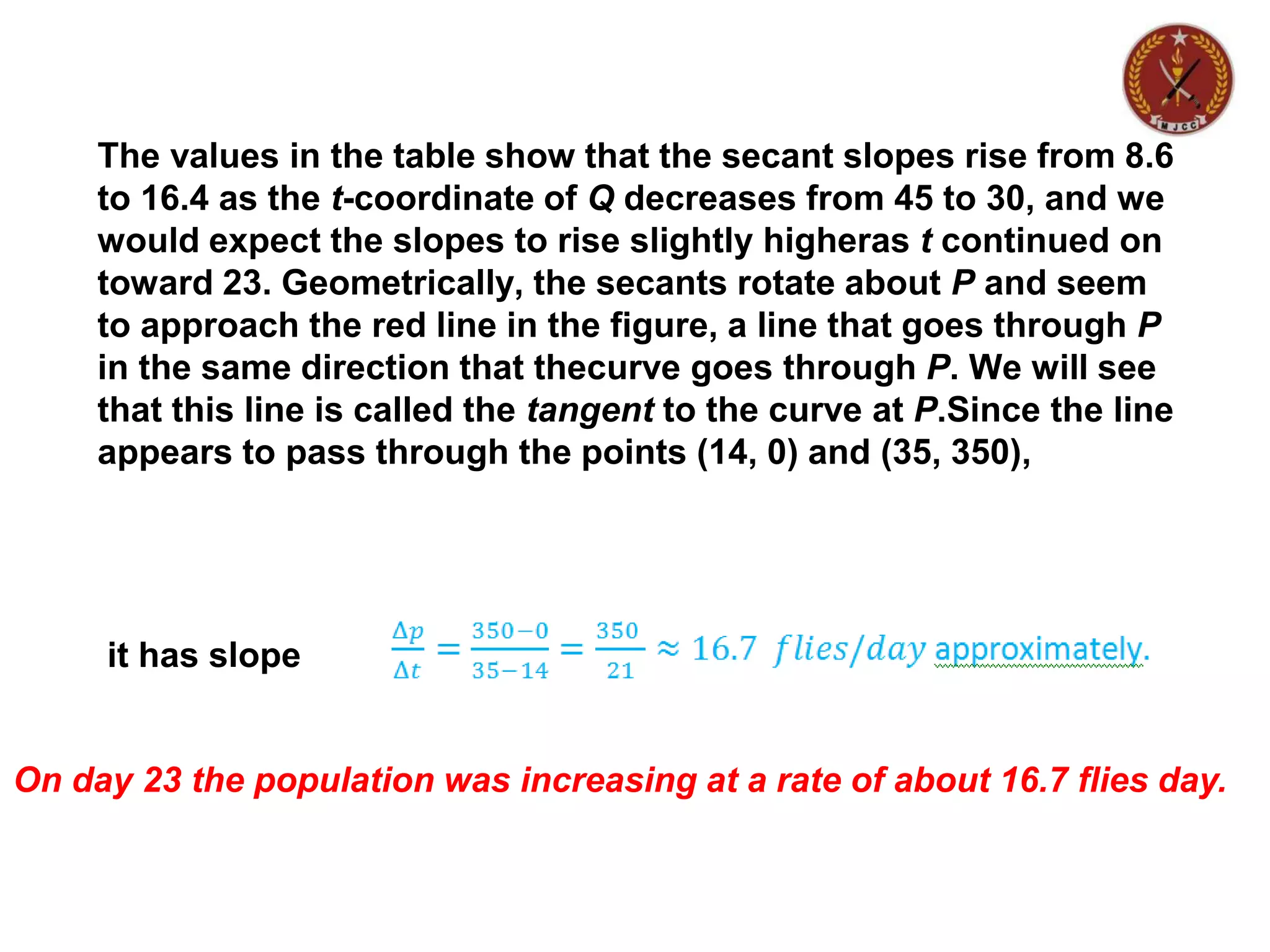
![Conclusion;
Geometrically, the rate of change of ƒ over [x1 x2], is the slope of
the line through the pointsP(x1,f(x1)) and Q(x2,f(x2)) Figure . In
geometry, a line joining two points of a curve is a secant to the
curve. Thus, the average rate of change of ƒ from x1 to x2 is
identical with the slope of secant PQ.
Experimental biologists often want to know the rates at which
populations grow undercontrolled laboratory conditions](https://image.slidesharecdn.com/hsscii-introductionoflimits-210810070258/75/Hssc-ii-introduction-of-limits-13-2048.jpg)
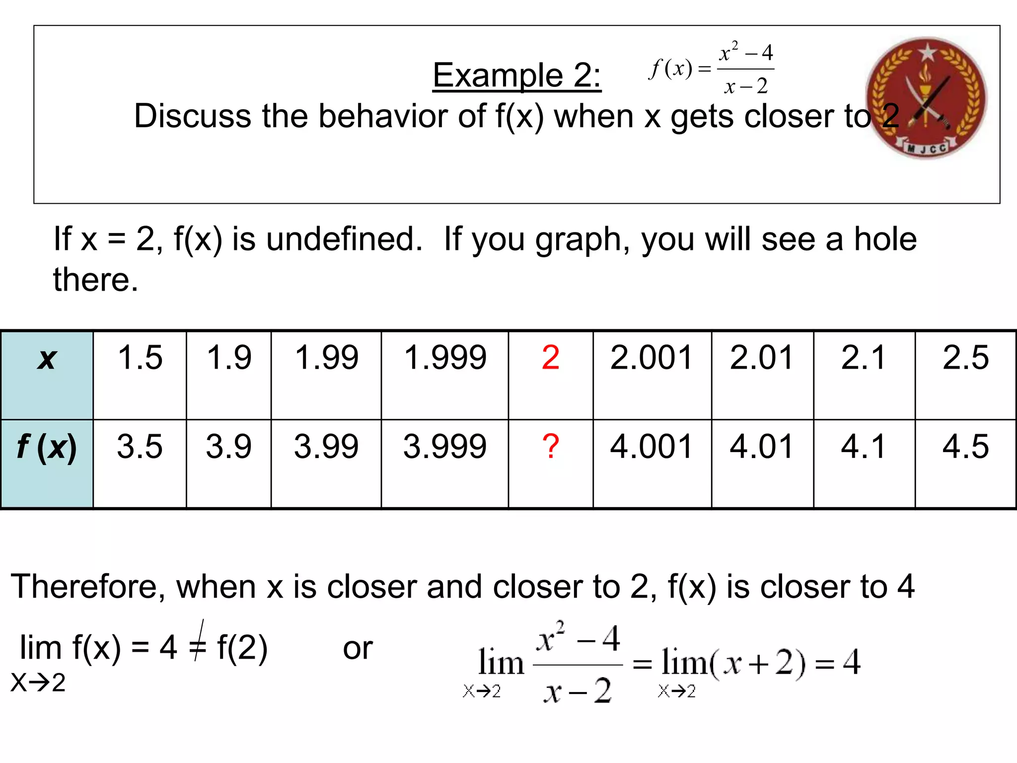
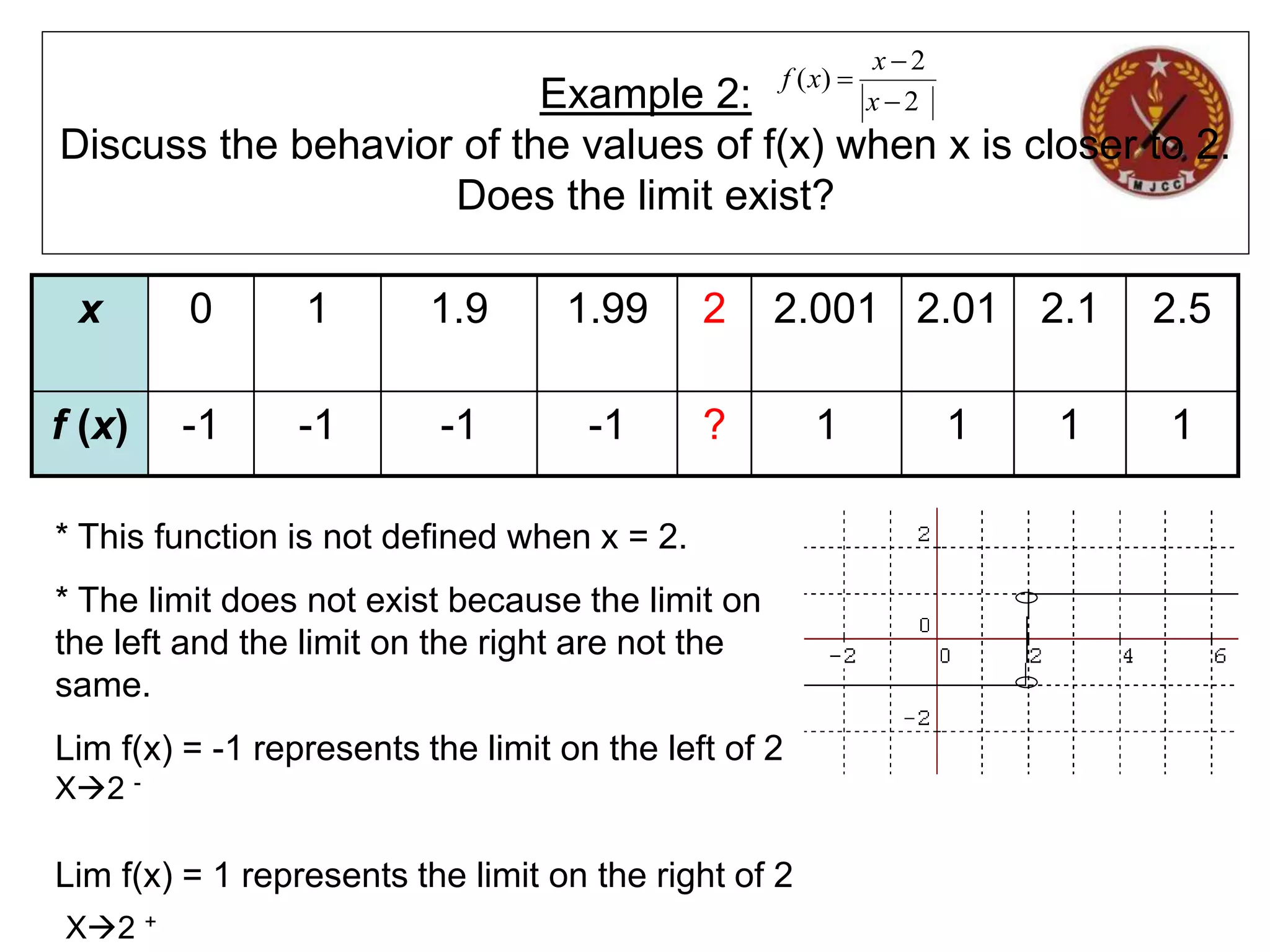
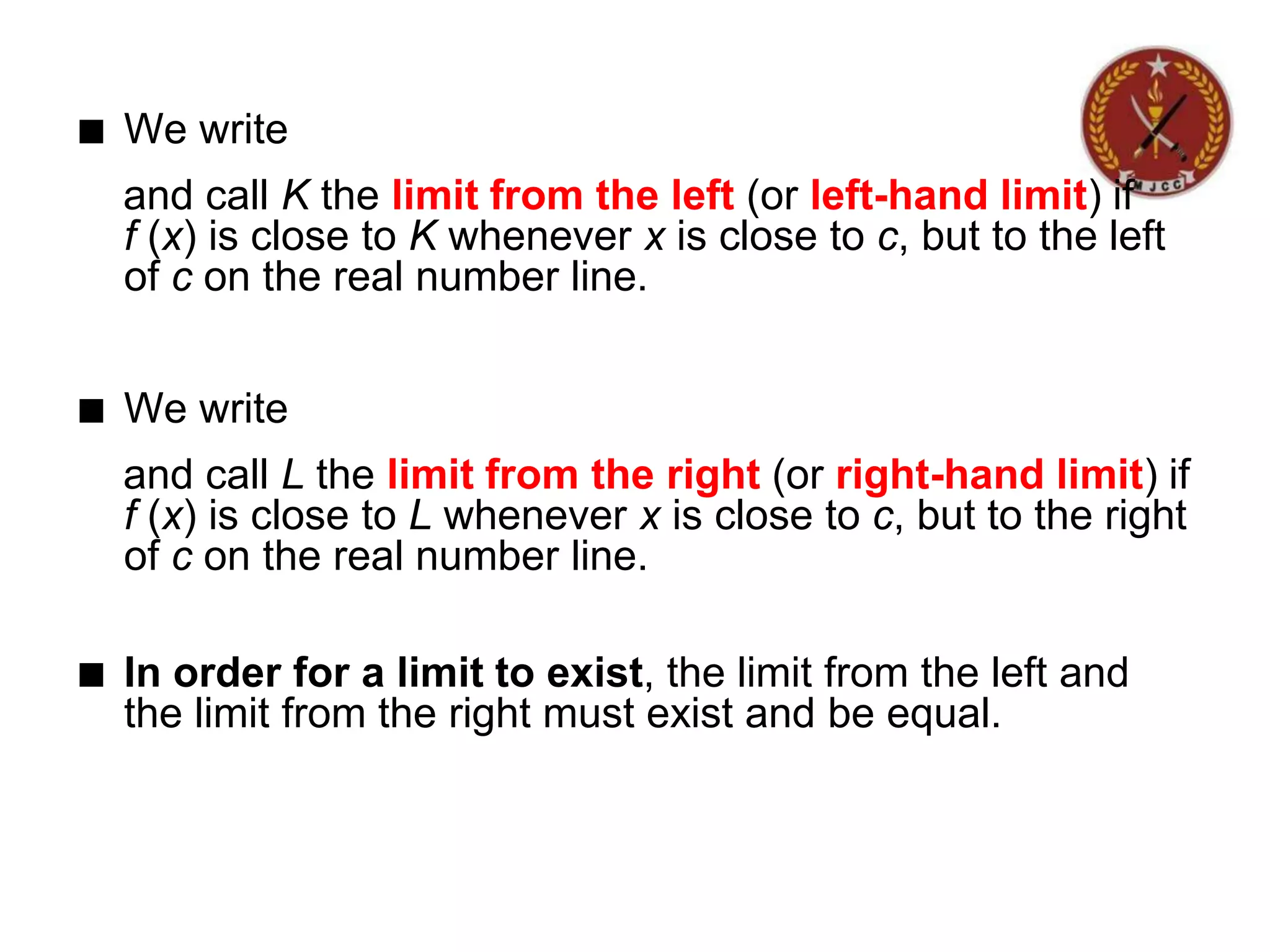
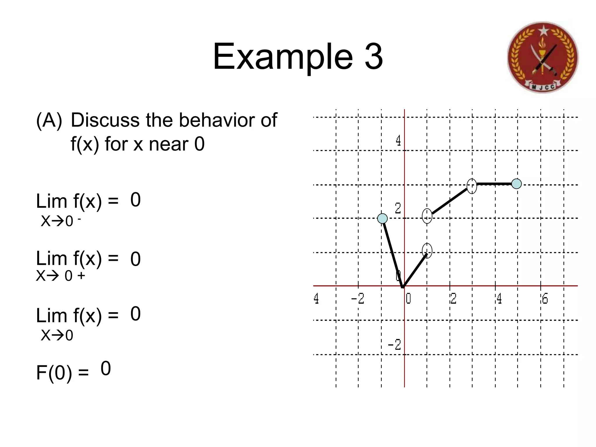
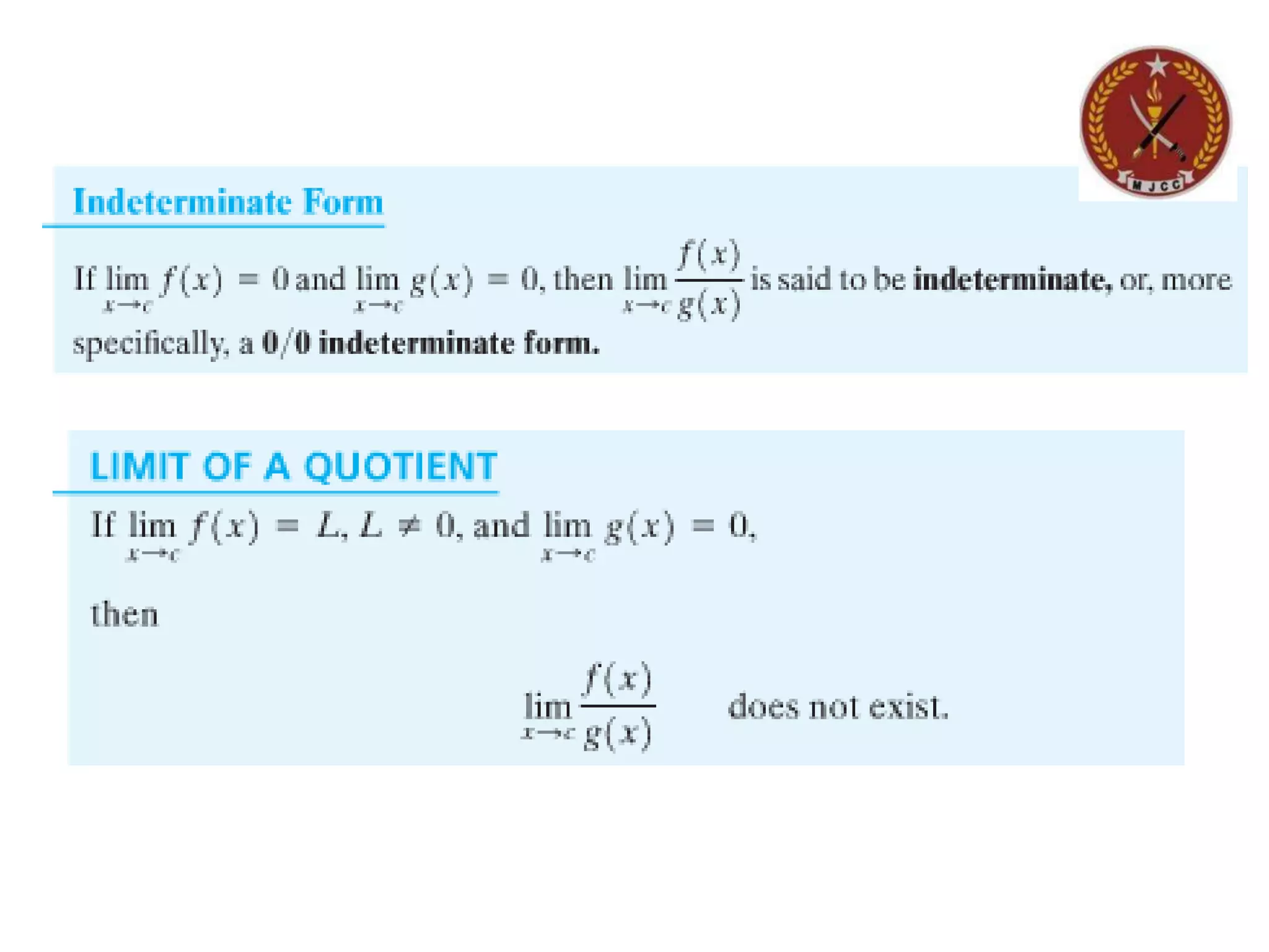
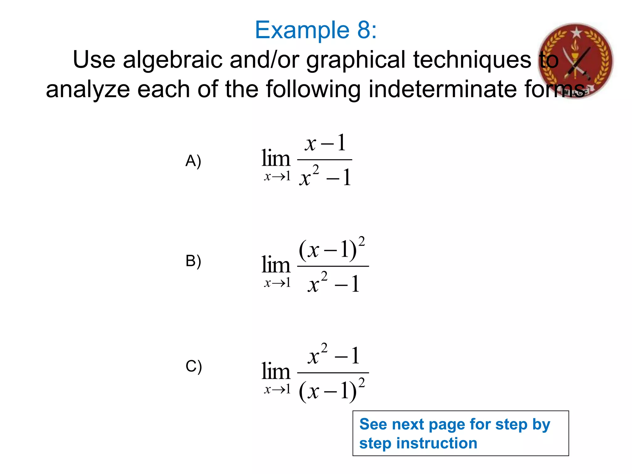
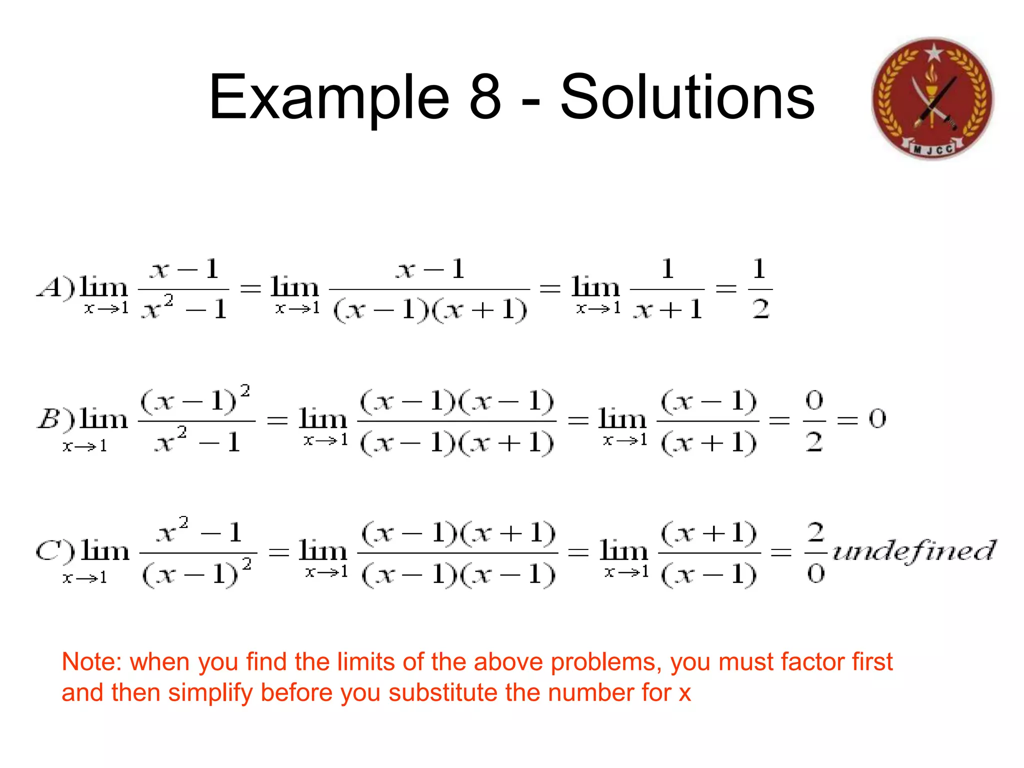
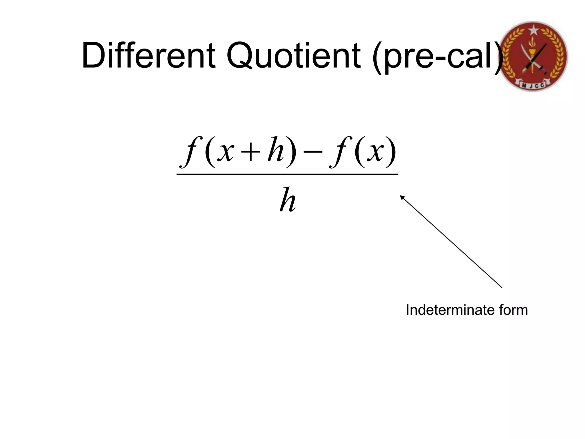
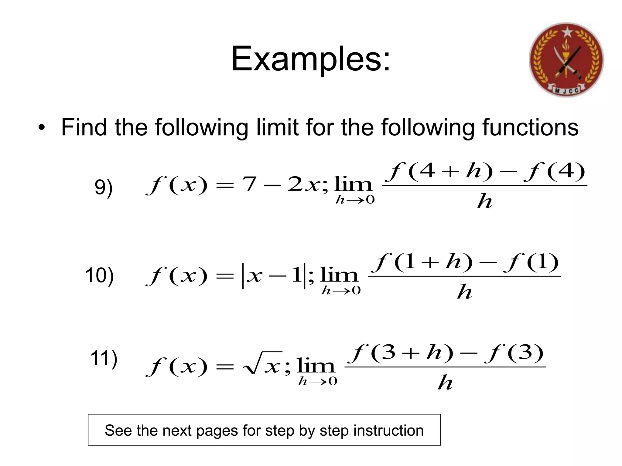


The document discusses limits of functions. It begins by defining key terms like "x approaches zero" and outlines learning outcomes related to limits. Examples are provided to illustrate calculating average and instantaneous rates of change using limits, as well as one-sided limits. The document explains that a limit exists only if the left-hand and right-hand limits are equal. Several examples demonstrate evaluating limits algebraically and graphically for various functions, including limits of rational functions. The document concludes by discussing indeterminate forms that arise when evaluating certain limits.