(1) The document discusses linear perturbations of the metric around a Schwarzschild black hole. It derives the Regge-Wheeler equation, which governs axial perturbations and takes the form of a wave equation with an effective potential. (2) It shows that the Regge-Wheeler potential has a maximum just outside the event horizon. This allows it to be considered as a scattering potential barrier for wave packets. (3) It concludes that Schwarzschild black holes are stable under smooth, compactly supported exterior perturbations, as these perturbations will remain bounded for all times according to properties of the Regge-Wheeler equation and solutions to the Schrodinger equation.

1. Hashiam Kadhim
Linearized Einstein Equations around the
Schwarzschild black hole
April 4, 2014

2. Contents
Introduction 1
Appropriate Metric 1
Cotton-Darboux Theorem 1
Perturbations of the Schwarzschild Black-Hole 3
Ricci Tensors 3
Metric Perturbations 4
Axial Perturbation of the Metric 4
Stability of the Schwarzschild Black-Hole 8
Summary 9
References 10

3. 1
(1)
(2)
Introduction
In their original work, Regge and Wheeler (1957) studied perturbations of the metric around a
Schwarzschild black hole [2]. Roughly speaking, this is done by introducing a perturbation
to the metric such that the new metric is:
where | | Thus, only terms linear in are retained in the calculations. Eventually, we
will show that a wave equation (named after Regge and Wheeler) with an effective potential
governs linear perturbations of a Schwarzschild black hole.
Appropriate Metric for Axisymmetric Spacetimes
Our principle concern is to be able to treat, in full generality, perturbations of axisymmetric
spacetimes. In order to do this, we must first find the metric in its most general form given the
conditions on our spacetime.
We start by taking two of our coordinates as the time t and the azimuthal angle ϕ
about the axis of symmetry. We study the case of space-times that retain their axisymmetry at all
times. This restrictions on our space-time requires that the coefficients of the contravariant form
of the metric
be independent of ϕ [1]. Our first goal is to show that the 3x3-matrix (where i,j = 0,2,3) can
be made into diagonal form by local coordinate transformation. This is done through the
application of the Cotton-Darboux theorem.
Cotton-Darboux Theorem
Theorem (Cotton-Darboux): the metric
in three dimensional space can always be brought to a diagonal form by a local
coordinate-transformation.

4. 2
(3)
(4)
(5)
(6)
Proof (taken from Chandrasekhar (1983) [1]):
Definition: a geodesic system of coordinates is constructed by considering a surface
such that , letting the geodesics, normal to , be the coordinate
lines , and choosing the coordinates on the surfaces geodesically parallel to f.
Now observe that by choice of geodesic system of coordinates, the metric can be brought to the
form:
{ }
Consider the coordinate transformation:
{ }
Where are functions of which we try to solve by condition that the metric (3) in the
new coordinate system is diagonal. This condition amounts to:
Or explicitly:
So,
( )
( )
( )
Now suppose that are functions of two variables , and are specified on the
surface (say ); and that are smooth and nowhere zero on the surface. Then

5. 3
(7)
(8)
(9)
(10)
(11)
(12)
(13)
by the Cauchy-Kowalewski theorem, there exists unique functions which satisfy the
system of equations (5) and which reduce to the values specified on the surface. The existence of
a local coordinate transformation which will bring the metric to the diagonal form is thus
established.
Thus, applying the Cotton-Darboux theorem to coordinates and assuming the
desirable coordinate transformation, we find that:
We don’t have to list all the coefficients due to the symmetry of the metric. We will write the
remaining coefficients to in the form:
where are functions of and [1]. Thus the covariant form the
metric obtained by lowering indices and writing each term of the metric out is of the form
Now we have obtained the general metric that we were looking for.
Perturbations of the Schwarzschild Black-Hole
Ricci Tensors for our metric
Our goal is to obtain the relevant perturbation equations by linearizing the field equations about
the Schwarzschild solution. The following Ricci tensors of our metric (11) will be useful in our
endeavors. In what follows, we use the notation that a comma signifies ordinary partial
differentiation. For example: .
These tensors are calculated by Chandrasekhar (1983) and are found to be [1]:
[( ) ( ) ]
[( ) ( ) ]

6. 4
(14)
(15)
(16)
(17)
(18)
(19)
Where
{ }
Metric Perturbations
In the unperturbed case, the metric corresponds to the Schwarzschild metric
( ) ( )
So we associate with r,θ respectively and the metric coefficients are:
When the metric (14) is perturbed by an external agent and only linear terms are kept:
 become first order quantities
 The functions experience linear increments respectively
It’s easy to see that a perturbation leading to non-vanishing values of is a different kind
of perturbation than one leading to increments in . More specifically, the first
kind induces a rotation of the black hole while the second kind does not because it is independent
of the sign of [2]. The first kind of perturbation will be referred to as axial, and the second
kind will be referred to as polar [1]. As it turns out, these two kinds of permutations decouple in
the sense that they can be considered independently of each other. Our interest in the Regge-
Wheeler equation leads us to study the axial perturbations.
Axial Perturbation of the Metric
The equations governing non-vanishing are given by
From (12,13) we see that we could plug in into and we get:
( )

7. 5
(20)
(21)
(22)
(23)
(24)
(25)
(26)
(27)
(28)
(29)
( )
Let
and substituting for their unperturbed values (16), we get:
( )
( )
Further, we assume harmonic time dependence of the perturbation where ω is generally a
real constant [2]. This corresponds to a Fourier component with frequency –ω when conducting
a Fourier analysis of the perturbation [1]. From this time dependence, we can re-write equations
(21) and (22) as [1]:
Eliminating from the previous two equations, we obtain:
( ) ( )
The variables r and θ in (25) can be separated by the substitution [1]:
Where denotes the Gegenbauer function governed by:
or
( )
Where are the Legendre polynomials. The substitution (26) into (25) we get the radial
equation [1]:
( )

8. 6
(30)
(31)
(32)
(33)
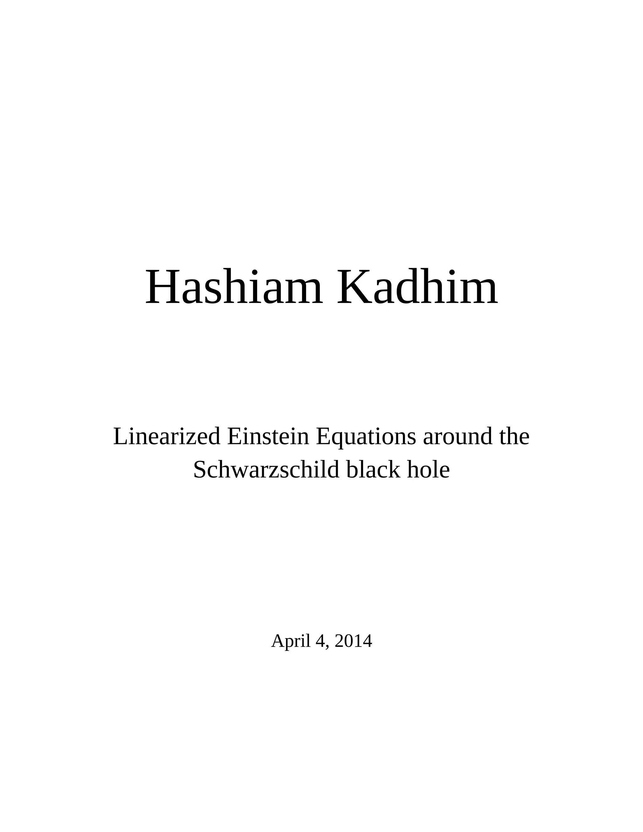
Changing to the tortoise coordinates [2]:
( )
which satisfies
( )
Letting:
[( ) ]
We find that satisfies the Schrodinger wave equation
( )
This is the Regge-Wheeler equation that governs the axial perturbations of Schwarzschild black
holes. The potential is referred to as the Regge-Wheeler potential. This potential has a
maximum just outside the event horizon r ~ 3.3M as shown in Figure 1 below [3].

9. 7
(34)
(35)
(36)
Because the Regge-wheeler equation satisfies the Schrodinger equation, we can assert that the
Regge-wheeler equation shares the well-known properties of a wave equation. We first assert
that the Regge-Wheeler potential V is positive everywhere and smooth. Further, the potential
decays at infinity. More specifically [1]:
Further, since V decays faster than , the asymptotic behavior of Z is given by:
For real ω, the solution represents ingoing and outgoing waves at .
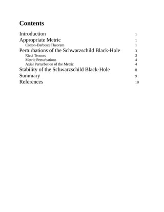
Figure 1 [3]
This graph shows the Regge-Wheeler potential vs. r/M. The maximum is seen to be around r ~
3.3M. Because the Regge-Wheeler satisfied the Schrodinger equation, the potential can be
thought of as a scattering potential barrier. Q represents an incoming wave packet from positive
spatial infinity; the other two wavy lines show the reflected and transmitted portion of the
incident wave packet.

10. 8
(37)
(39)
(38)
The Regge-Wheeler potential can be thought of as a scattering potential [3] as in quantum
mechanics. Figure 1 above depicts an incident wave packet Q originating from positive spatial
infinity interacting with the scattering potential barrier (in this case the Regge-Wheeler
potential). Some of the wave packet is transmitted and the rest is reflected.
Stability of the Schwarzschild Black Hole
The question we wish to answer in this section is the following: given an initial smooth
perturbation with a compact support in the exterior region of the black hole, will it remain
bounded at all times as it evolves?
We shall take for granted that the linearized equations of polar perturbations of a Schwarzschild
black hole are of the form (33), just with a different effective potential. This was derived by
Zerilli and is known as the Zerilli equation [2].
The solution comes from elementary quantum theory. The properties we have explored of the
potential imply that it is integrable (since it’s smooth and decays fast enough). Theorems from
quantum theory guarantee that the wave functions belonging to any observable form a complete
set, and that any square integrable function that can describe a state of the system can be
expanded in terms of them, and further, that the integral of the absolute square of any state
function must remain constant with time [1].
We have seen that perturbations of the Schwarzschild black hole are governed by the 1-
dimensional wave equation
( )
With asymptotic behavior
The solutions to equation (36), satisfying (37) provide the basic complete set of wave
functions [1]. Therefore any smooth compactly supported exterior perturbation can be expressed
as an integral over the functions in the form [1]:
√
∫ ̂
Therefore, from quantum theory, the evolved perturbation is expressed by:

11. 9
(40)
(41)
√
∫ ̂
Thus, from the following:
∫ ∫ ̂ ∫
we assert that the perturbation is bounded for all times which implies the stability of the
Schwarzschild black hole for smooth compactly supported exterior perturbations.
Summary
We started with the task of finding a suitably general metric. After obtaining this metric, we
applied a small linear axial perturbation to it. After doing this, we found the linearized Einstein
field equations around a Schwarzchild black hole. The resulting Regge-Wheeler equation turns
out to satisfy the Schrodinger equation and therefore has nice properties that we know from the
study of solutions to the Schrodinger equation. Finally, smooth compactly supported exterior
perturbations will remain bounded, therefore implying that Schwarzschild black holes are stable
under such perturbations.

12. 10
References
[1] Chandrasekhar S. The mathematical theory of black holes
[2] V. Frolov, I. Novikov. Black Hole Physics: Basic Concepts and New Developments
[3] L. Rezolla. Gravitational Waves from Perturbed Black Holes and Relativistic Stars