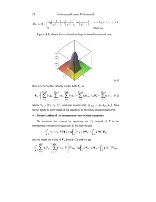
This document presents the mathematical modeling of heat transfer and phase change in three dimensions using the finite element method. It begins with the governing equations - the continuity, Navier-Stokes, and heat equations along with the Stefan free boundary condition. It then derives the variational formulation and discretizes the equations using finite elements. The nonlinear system is solved using Newton's method to find the numerical solution for temperature, velocity, and the moving solid-liquid interface over time.

1. Advances and Applications in Fluid Mechanics
© 2016 Pushpa Publishing House, Allahabad, India
Published Online: December 2015
http://dx.doi.org/10.17654/FM019010023
Volume 19, Number 1, 2016, Pages 23-34 ISSN: 0973-4686
Received: May 20, 2015; Accepted: July 6, 2015
2010 Mathematics Subject Classification: 76A02.
Keywords and phrases: heat transfer, Navier-Stokes, finite element method, Stefan condition.
Communicated by Shahrdad G. Sajjadi
MATHEMATICAL MODELING OF HEAT
TRANSFER AND TRANSPORT PHENOMENA IN
THREE-DIMENSION WITH STEFAN FREE BOUNDARY
Mohammad Hassan Mohammadi
Institute of Mathematics
National Academy of Sciences of Republic of Armenia
Armenia
e-mail: mohamadi.mh.edu@gmail.com
Abstract
In this paper, we state the mathematical modeling of heat transfer in
the furnaces in the three-dimensional case. This modeling consists of
the continuity equation, the Navier-Stokes equations, and the heat
equation with the free boundary Stefan condition. We derive the
variational formulation of the equations, and we invoke the finite
element method technique to get the numerical solution of the system.
1. Introduction
Mathematical modeling of glass melting and heat transfer is one of
the basic tools to analyze the melting and freezing process. It helps to
the engineers to optimize the process of melting and freezing, and even
in furnace design stage, and the other approaches are much more expensive
[1-3]. Many researchers prepared the different techniques to find the

2. Mohammad Hassan Mohammadi24
mathematical modeling and solution of the melting and freezing process
[4-6].
In this work, we express the mathematical modeling of melting process
in the Garnisazh furnace for the Newtonian fluid. The melted material inside
the furnace in the center part has very high temperature, but the material near
the body of the furnace does not get enough heat, then it is going to be solid.
The boundary between the liquid and solid material is moving all the time,
and it is unknown for us, then the geometry, velocity, and the behavior of
the free boundary are unknown too. Prediction of the behavior of the free
boundary is very important during the melting process and it is necessary to
use it in the modeling process of glass melting. Stefan condition is the
convenient model for the free boundary between solid and liquid material
[9, 10], then we will use it in our work.
After deriving the strong formulation of melting process, we convert all
of the equations to the weak formulation and then we invoke the finite
element method to find the numerical solution of the system. The system that
is introduced in the numerical approach would be nonlinear, thus, we use the
Newton method to transfer the nonlinear system into a linear and every
classical method can be used to find the solution of the linear system.
2. Mathematical Modeling
We start the modeling of changing the phase from solid to liquid in
three-dimension [1, 2, 4, 5], and we assume that the flow is Newtonian.
Also, suppose that the material occupying the bounded domain 3
R⊂Ω that
separated to two phases, the solid phase
{ },0<θ|θ=S
the liquid phase
{ },0>θ|θ=L
and the free boundary between the solid and liquid phase
{ }.0=θ|θ=Φ

3. Mathematical Modeling of Heat Transfer … 25
The strong formulation of the Stefan problem with convection is as
( ) 0=θ∆−θ∇⋅V in ,LS ∪ (2.1)
[ ] txx nλ=⋅λ−=⋅θ∇ +
− nwn on ,Φ (2.2)
where ( )tx n,n is the normal vector to the free boundary ,Φ w is the
velocity of the free boundary, and 0>λ is the latent heat.
Assume that
0=θ on ,Ω∂
0=V in ,S
and
0=⋅∇ V in ,L (2.3)
( ) ( )θ=∇+⋅∇−∇⋅ fVV pτ in ,L (2.4)
where ( )ijτ=τ is the viscous stress tensor, p is the pressure, and ( )θf is
the density of forces. For the incompressible flow, we have
,





∂
∂
+
∂
∂
µ=τ
i
j
j
i
ij x
u
x
u
and the Navier-Stokes equations (2.4) for an incompressible flow can be
restated as
( ) ( ).θ=∇+∆µ−∇⋅ fVVV p (2.5)
We also assume that
0=V on ( ) .SL ∪∪ Φ∂
All the equations and the boundary conditions describe the transport
phenomena in the mechanic of fluids, and these equations express the
mathematical modeling and the strong formulation of the transport
phenomena.

4. Mohammad Hassan Mohammadi26
3. Variational Formulation
In this part, we get the variational (weak) formulation of the transport
phenomena [9, 10], we start the converting by the heat equation (energy
conservation law), then we refer to the continuity equation (mass
conservation law), and finally we derive the weak formulation of the Navier-
Stokes equations (momentum conservation law).
3.1. Heat equation
We multiply the heat equation (2.1) by ,η and integrate the equality over
the domain ,Ω then
( )∫ ∫Ω Ω
=θη∆−θ∇⋅η ,0V
where ( ),1
0 Ω∈η H and ( )Ω1
0H is the Sobolev space. Integration by parts
and the Green’s first identity imply that
( ) ([ ] )∫ ∫ ∫Ω Ω Φ
+
− η⋅θ∇=η∇⋅θ∇+η∇⋅θ− .xnV (3.1)
Define the function H as
( )



≤θ
>θλ−
=θ
,0;0
,0;
H
then by integrating the Stefan condition (2.2), we get
([ ] ) ( ) ( )∫ ∫ ∫ ∫Φ Φ Ω
+
− η∇⋅θ=η∇⋅λ−=η⋅λ−=η⋅θ∇
L
,wwnwn Hxx (3.2)
then by using (3.2), we rewrite the relation (3.1) as
( ) ( )∫ ∫ ∫Ω Ω Ω
=η∇⋅θ∇−η∇⋅θ+η∇⋅θ .0VwH (3.3)
3.2. Continuity equation
Now we focus on the continuity equation (2.3) by the same approach to
get the integral equation

5. Mathematical Modeling of Heat Transfer … 27
( )∫ =ξ⋅∇
L
,0V
where ( ),1
0 LH∈ξ then integration by parts leads to the integral equation
∫ =ξ∇⋅
L
.0V (3.4)
3.3. Navier-Stokes equations
In the final part, we want to compute the variational formulation of the
Navier-Stokes equations (2.5) for an incompressible flow
( ) ( )∫ ∫ ∫ ∫ ⋅θ=⋅∇+⋅∆µ−∇⋅⋅
L L L L
,ΨΨΨΨ fVVV p (3.5)
where ( ( )) .31
0 LH∈Ψ Assume that the pressure is constant in the liquid
zone, and by using the integration by parts and the Green’s first identity we
will get
( ) ( )∫ ∫ ∫ ⋅θ=µ+∇⋅⋅−
L L L
,: ΨΨΨ fVVV DD (3.6)
where
∑∑
= =
∂
ψ∂
∂
∂
=
3
1
3
1
.:
i j
j
i
j
i
xx
u
DD ΨV
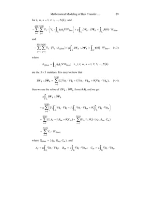
4. Discretization of the Domain
We start the finite element method by the discretization of the domain Ω
[15-17], and for this aim suppose that ( )hhhh wvu ,,=V is the velocity
vector field in the finite dimensional space ,hS where
{ ( )} ( ),dim,...,,,, 321 hNspan hhNh =φφφφ= SS
and the basis test functions ( ),,, zyxiφ ( ),...,,2,1 hNi = have small
support. We select the test functions iφ as

6. Mohammad Hassan Mohammadi28
( )





<<<





−







−






−=φ
otherwise.0
,1,1,1
1
1
exp
1
1
exp
1
1
exp
,, 222
zyx
zyxzyx
Figure (4.1) shows the test function shape in two-dimensional case
(4.1)
then we rewrite the velocity vector field hV as
( )( )( )
( )
( )( )
∑ ∑∑ ∑ ∑
= == = =
φ=φ=








φφφ=
hN
i
hN
i
iiiiii
hN
i
hN
i
hN
i
iiiiiih WVUWVU
1 11 1 1
,,,,, VV (4.2)
where ( ),,, iiii WVU=V and also assume that ( ).,, nmllmn φφφ=W Now
we are ready to convert all of the equations to the finite dimensional form.
4.1. Discretization of the momentum conservation equations
We continue the process by replacing the hV instead of V in the
momentum conservation equations (3.6), then we get
( ) ( )∫ ∫ ∫ ⋅θ=µ+∇⋅⋅−
L L L
,: hhhhhh DD ΨΨΨ fVVV
and we insert the value of hV from (4.2), and we get
( )
( )
( )
∫ ∑ ∫ ∫∑
= =
⋅θ=µ+








∇⋅φ⋅φ−
L L L
hN
i
lmnhhlmn
hN
j
jjii DD
1 1
,: WWVV fV Ψ

7. Mathematical Modeling of Heat Transfer … 29
for ( ),...,,3,2,1,, hNnml = and
( )
( )( )
∑ ∑ ∫ ∫∫= =
⋅θ=µ+





∇φφ⋅⋅−
hN
i
hN
j
lmnhhlmnjiii DD
1 1
,:
L LL
WWVV fV Ψ
and
( ) ( )
( )( )
∑ ∑ ∫ ∫= =
⋅θ=µ+⋅⋅−
hN
i
hN
j
lmnhhijlmnii DD
1 1
,:
L L
WAVV fV Ψ (4.3)
where
( )∫ =∇φφ=
L
hNnmljilmnjiijlmn ...,,3,2,1,,,,;WA
are the 33 × matrices. It is easy to show that
( )
( )
∑
=
φ∇⋅φ∇+φ∇⋅φ∇+φ∇⋅φ∇=
hN
i
niimiiliihh WVUDD
1
,: ΨV (4.4)
then we use the value of hh DD Ψ:V from (4.4), and we get
∫µ
L
hh DD Ψ:V
( )
∑ ∫ ∫ ∫=






φ∇⋅φ∇+φ∇⋅φ∇+φ∇⋅φ∇µ=
hN
i
niimiilii WVU
1
L L L
( ) ( ) ( )
( )( )
∑ ∑
= =
⋅=++=
hN
i
hN
i
inimiliiiiniimiili CBAWVUCWBVAU
1 1
,,,,
( )
∑
=
⋅=
hN
i
ilmni
1
,WV
where ( ),,, inimililmn CBA=Q and
∫ ∫ ∫ φ∇⋅φ∇µ=φ∇⋅φ∇µ=φ∇⋅φ∇µ=
L L L
,;; niinmiimliil CBA

8. Mohammad Hassan Mohammadi30
then we have
( )
∫ ∑
=
⋅=µ
L
hN
j
ilmnihh DD
1
.: QVΨV (4.5)
Now, by invoking (4.5), we are in the position that to rewrite the equality
(4.3) as
( )
( )( )( )
∑ ∑ ∑
= = =
=⋅−⋅⋅
hN
i
hN
j
hN
i
lmnilmniijlmnji
1 1 1
,FQVAVV (4.6)
where
( )∫ ⋅θ−=
L
.lmnlmn WF f
4.2. Discretization of the mass conservation equation
We continue the process by referring to the continuity equation and
replacing the hV into (3.4) and we have
∫ =ξ∇⋅
L
,0hhV (4.7)
then we express it as
( )
( )( )
∫ ∑ ∑ ∫= =
==φ∇φ⋅=φ∇⋅φ
L L
hN
i
hN
i
jiijii hNj
1 1
,...,,3,2,1;0VV (4.8)
then we derive
( )
( )
∑
=
==⋅
hN
i
iji hNj
1
,...,,3,2,1;0BV (4.9)
where
∫ φ∇φ=
L
.jiijB

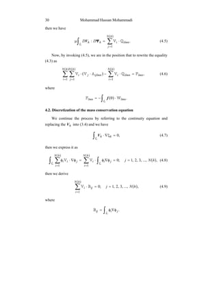
9. Mathematical Modeling of Heat Transfer … 31
4.3. Discretization of the energy conservation equation
In the final part, we focus on weak formulation of the heat equation (3.3)
and we get
( ) ( )
( )( )
∫ ∫ ∑ ∫ ∑Ω Ω
=
Ω
=
=φ∇⋅φθ+φ∇⋅φ∇θ−φ∇⋅θ
hN
i
hN
i
jiijiijH
1 1
,0Vw (4.10)
then we restate it as
( ) ( ( ) )
( )
∫ ∑ ∫Ω
=
Ω
=φ∇⋅φ−φ∇⋅φ∇θ−φ∇⋅θ
hN
i
jijiijH
1
,0Vw (4.11)
thus we have
( )
( )
∑
=
==θ
hN
i
jiji hNj
1
,...,,3,2,1;DC (4.12)
where
( ( ) ) ( )∫ ∫Ω Ω
φ∇⋅θ=φ∇⋅φ−φ∇⋅φ∇= .; jjjijiij H wV DC
4.4. Imposing the Stefan condition
Now the problem is how we can find w, the velocity of the free
boundary, for solving the problem we will use variational version of the
Stefan condition (3.2), it is easy to show that
([ ] ) ( ) ( )∫ ∫ ∫ ∫ ∫Φ Φ Φ
+
− ∂
η∂
θ=
∂
η∂
λ=ηλ=η⋅λ−=η⋅θ∇
L Q
,
t
H
t
ntxx nwn
where ( ),,0 T×Ω=Q then we will have
( ) ( ) ( )∫ ∫ ∫Φ ∂
η∂
θ
λ
−=η=η⋅
L Q
,
1
t
Hdivx wnw (4.13)
and we get
( ) ( )∫ ∫Ω ∂
φ∂
θ
λ
−=φ∇⋅θ=
Q
.
1
t
HH
j
jj wD (4.14)

10. Mohammad Hassan Mohammadi32
Note that for computing the ,jD we need to assume that ( ),, txjj φ=φ
where ( ) ., Q∈tx
5. Summary and Results
The purpose of this article is to prepare the approach to get the numerical
solution of the transport phenomena in the mechanic of fluids. For this aim,
we started by the mathematical modeling of the transport phenomena, and we
stated the three important equations, that is, the heat equation, the continuity
equation, and the Navier-Stokes equations. Also, we took some convenient
boundary conditions, especially the Stefan condition that it is the best
modeling for the moving boundary between the liquid and solid zones, and
we imposed the Stefan condition into the heat equation.
During the process, we got the variational formulation of the equations
because we wanted to apply the finite element method to achieve the
numerical solution of the nonlinear system. Finally, by discretization of the
solution space and equations, we derived the following system:
( ) ( )
( )( )( )
,...,,3,2,1,,;
1 1 1
∑ ∑ ∑
= = =
==⋅−⋅⋅
hN
i
hN
j
hN
i
lmnilmniijlmnji hNnmlFQVAVV
( )
( )
,...,,3,2,1;0
1
∑
=
==⋅
hN
i
iji hNjBV
( )
( )
∑
=
==θ
hN
i
jiji hNj
1
,...,,3,2,1;DC
where all the coefficients could be determined.
The first system is nonlinear and the Newton’s method is recommended
to solve the system, the second and the third are linear and they are solvable
by any classical approach for linear systems, then we reach our purpose to
find the numerical solution of the transport system.

11. Mathematical Modeling of Heat Transfer … 33
References
[1] A. Ungan and R. Viskanta, Three-dimensional numerical modeling of circulation
and heat transfer in a glass melting tank, IEEE Transactions on Industry
Applications IA-22(5) (1986), 922-933.
[2] A. Ungan and R. Viskanta, Three-dimensional numerical simulation of circulation
and heat transfer in an electrically boosted glass melting tank. Part 2. Sample
simulations, Glastechnische Berichte 60(4) (1987), 115-124.
[3] S. Yu. Sadov, P. N. Shivakumar, D. Firsov, S. H. Lui and R. Thulasiram,
Mathematical model of ice melting on transmission lines, Journal of Mathematical
Modeling and Algorithms 6(2) (2007), 273-286.
[4] L. Pilon, G. Zhao and R. Viskanta, Three-dimensional flow and thermal structures
in glass melting furnaces. Part I. Effects of the heat flux distribution, Glass
Science and Technology 75(2) (2002), 55-68.
[5] L. Pilon, G. Zhao and R. Viskanta, Three-dimensional flow and thermal structures
in glass melting furnaces. Part II. Effect of batch and bubbles, Glass Science and
Technology 75(3) (2006), 115-124.
[6] Manoj K. Choudhary, Raj Venuturumilli and Matthew R. Hyre, Mathematical
modeling of flow and heat transfer phenomena in glass melting, delivery, and
forming processes, International Journal of Applied Glass Science 1(2) (2010),
188-214.
[7] V. Alexiades and A. D. Solomon, Mathematical Modeling of Melting and
Freezing Processes, Hemisphere Publishing Corporation, 1993.
[8] Henry Hu and Stavros A. Argyropoulos, Mathematical modelling of solidification
and melting: a review, Modelling and Simulation in Materials Science and
Engineering 4 (1996), 371-396.
[9] J. F. Rodrigues, Variational methods in the Stefan problem, Lecture Notes in
Mathematics, Springer-Verlag, 1994, pp. 147-212.
[10] C. Vuik, A. Segal and F. J. Vermolen, A Conserving Discretization for a Stefan
Problem with an Interface Reaction at the Free Boundary, Computing and
Visualization in Science, Springer-Verlag, Vol. 3, 2000, pp. 109-114.
[11] R. Byron Bird, Warren E. Stewart and Edwin N. Lightfoot, Transport Phenomena,
2nd ed., John Wiley & Sons, Inc., 2002.
[12] Irving H. Shames, Mechanics of Fluids, 4th ed., McGraw-Hill, 2003.

12. Mohammad Hassan Mohammadi34
[13] Robert W. Fox, Alan T. McDonald and Philip J. Pritchard, Introduction to Fluid
Mechanics, 6th ed., John Wiley & Sons, Inc., 2004.
[14] Xu Quan-Sheng and Zhu You-Lan, Solution of the two-dimensional Stefan
problem by the singularity-separating method, Journal of Computational
Mathematics 3(1) (1985), 8-18.
[15] S. Brenner and R. Scott, The Mathematical Theory of Finite Element Methods,
Springer-Verlag, 1994, Corr. 2nd printing 1996.
[16] C. Johnson, Numerical Solution of Partial Differential Equations by the Finite
Element Method, CUP, 1990.
[17] James F. Epperson, An Introduction to Numerical Methods and Analysis, John
Wiley & Sons, Inc., 2002.
[18] K. Eriksson, D. Estep, P. Hansbo and C. Johnson, Computational Differential
Equations, CUP, 1996.
[19] V. Kambourova and I. Zheleva, Temperature distributions in a tank of glass
melting furnace, Comptes Rendus de L’Academie Bulgare des Sciences
55(8) (2002), 41-46.
[20] S. Patankar, Numerical Heat Transfer and Fluid Flow, Hemisphere, Washington,
DC, 1980.