This document provides an overview of starting SPSS and entering data. It discusses starting SPSS, defining variables, entering data for sample students, saving data files, and loading data files. Key steps include defining variables in the Variable View window by naming them and adding value labels, entering data horizontally in the Data View window, and saving files with a .sav extension so they can be opened later in SPSS.

1. A Step-by-Step Guide
to Analysis and Interpretotion
Brian C. Cronk
ll
I
L
:,-

2. ChoosingtheAppropriafeSfafistical lesf
Ytrh.t b Yq
I*l
QraJoi?
Dtfbsr
h
ProportdE
Mo.s Tha 1
lnd€Fndont
Varidl6
lldr Tho 2 L6Eb
d li(bsxlq*
Vdidb
lhre Thsn 2 L€wls
of Indop€nddtt
Varisd€
f'bre Tha 'l
Indopadqrl
Vdbue
'|
Ind.Fddrt
Vri*b
fro.! Itn I
l.doFfihnt
Vdi.bb
NOTE:Relevantsectionnumbersare
giveninparentheses.Forinstance,
'(6.9)"refersyouto Section6.9in
Chapter6.
I

3. Notice
SPSSis a registeredtrademarkof SPSS,Inc.Screenimages@by SPSS,Inc.
andMicrosoftCorporation.Usedwith permission.
Thisbookis not approvedor sponsoredby SPSS.
"PyrczakPublishing"isanimprintof FredPyrczak,Publisher,A CaliforniaCorporation.
Althoughtheauthorandpublisherhavemadeeveryefforttoensuretheaccuracyand
completenessof informationcontainedin thisbook,weassumenoresponsibilityfor
errors,inaccuracies,omissions,or anyinconsistencyherein.Any slightsof people,
places,or organizationsareunintentional.
ProjectDirector:MonicaLopez.
ConsultingEditors:GeorgeBumrss,JoseL. Galvan,MatthewGiblin,DeborahM. Oh,
JackPetit.andRichardRasor.
Editdrialassistanceprovidedby CherylAlcorn,RandallR.Bruce,KarenM. Disner,
BrendaKoplin,EricaSimmons,andSharonYoung.
Coverdesignby RobertKiblerandLarryNichols.
Printedin theUnitedStatesof AmericabyMalloy,Inc.
Copyright@2008,2006,2004,2002,1999byFredPyrczak,Publisher.All rights
reserved.No portionof thisbookmaybereproducedor transmittedin anyformorby any
meanswithoutthepriorwrittenpermissionof thepublisher.
rsBNl-884s85-79-5

4. Tableof Contents
IntroductiontotheFifthEdition
What'sNew?
Audience
Organization
SPSSVersions
Availabilityof SPSS
Conventions
Screenshots
PracticeExercises
Acknowledgments'/
ChapterI GettingStarted
Ll
t.2
1.3
1.4
1.5
1.6
1.7
Chapter2 EnteringandModifyingData
StartingSPSS
EnteringData
DefiningVariables
LoadingandSavingDataFiles
RunningYourFirstAnalysis
ExaminingandPrintingOutputFiles
Modi$ingDataFiles
VariablesandDataRepresentation
TransformationandSelectionof Data
Chapter3 DescriptiveStatistics
3.1
3.2
3.3
3.4
3.5
Chapter4 GraphingData
FrequencyDistributionsandpercentileRanksfor a singlevariable
FrequencyDistributionsandpercentileRanksfor Multille variables
Measuresof CentralTendencyandMeasuresof Dispersion
foraSingleGroup
Measuresof CentralTendencyandMeasuresof Dispersion
for MultipleGroups
StandardScores
4l
4l
43
45
49
2.1
') ')
v
v
v
v
vi
vi
vi
vi
vii
vii
I
I
I
2
5
6
8
ll
ll
t2
l7
t7
20
24
)7
29
29
29
3l
33
36
39
2l
Chapter5 PredictionandAssociation
4.1
4.2
4.3
4.4
4.5
4.6
5.1
5.2
5.3
5.4
GraphingBasics
TheNewSPSSChartBuilder
BarCharts,PieCharts,andHistograms
Scatterplots
AdvancedBarCharts
EditingSPSSGraphs
PearsonCorrelation Coefficient
SpearmanCorrelation Coefficient
SimpleLinear Regression
Multiple LinearRegression
u,

5. Chapter6
6.1
6.2
6.3
6.4
6.5
6.6
6.7
6.8
6.9
6.10
Chapter7
7.1
7.2
7.3
7.4
7.5
7.6
Chapter8
8.1
8.2
8.3
8.4
AppendixA
AppendixB
ParametricInferentialStatistics
Reviewof BasicHypothesisTesting
Single-Samplet Test
Independent-SamplesI Test
Paired-Samplest Test
One-WayANOVA
FactorialANOVA
Repeated-MeasuresANOVA
Mixed-DesignANOVA
Analysisof Covariance
MultivariateAnalysisof Variance(MANOVA)
NonparametricInferentialStatistics
Chi-SquareGoodnessof Fit
Chi-SquareTestof Independence
Mann-WhitneyUTest
WilcoxonTest
Kruskal-Wallis,F/Test
FriedmanTest
TestConstruction
Item-TotalAnalysis
Cronbach'sAlpha
Test-RetestReliability
Criterion-RelatedValidiw
EffectSize
PracticeExerciseDataSets
PracticeDataSetI
PracticeDataSet2
PracticeDataSet3
Glossary
SampleDataFilesUsedin Text
COINS.sav
GRADES.sav
HEIGHT.sav
QUESTIONS.sav
RACE.sav
SAMPLE.sav
SAT.sav
OtherFiles
Informationfor Usersof EarlierVersionsof SPSS
GraphingDatawithSPSS13.0and14.0
53
53
))
58
6l
65
69
72
75
79
8l
85
85
87
.90
93
95
97
99
99
100
l0l
t02
103
r09
109
ll0
ll0
lt3AppendixC
AppendixD
AppendixE
AppendixF
tt7
n7
ll7
ll7
n7
l18
l18
lt8
lt8
l19
t2l
tv

6. ChapterI
Section1.1 StartingSPSS
ffi$t't****
ffi
c rrnoitllttt
(- lhoari{irgqrory
r,Crcrt*rsrcq.,y urhgDd.b6.Wbrd
(i lpanrnaridirgdataura
f- Dml*ro* fe tf*E h lholifrra
GettingStarted
Startup proceduresfor SPSSwill differ
slightly,dependingon the exactconfigurationof
the machineon which it is installed.On most
computers,you can start SPSSby clicking on
Start, then clicking on Programs,then on SPSS.
On many installations,therewill be an SPSSicon
on the desktopthat you can double-clickto start
theprogram.
When SPSSis started,you may be pre-
sentedwith the dialog box to the left, depending
on theoptionsyour systemadministratorselected
for your versionof the program.If you havethe
dialog box, click Type in data and OK, which
will presenta blankdata window.'
If you were not presentedwith the dialog
box to the left, SPSSshouldopenautomatically
with a blankdata window.
The data window and the output win-
dow provide the basic interface for SPSS. A
blankdata window is shownbelow.
Section1.2 EnteringData
One of the keys to success
with SPSSis knowing how it stores
and usesyour data.To illustratethe
basicsof data entry with SPSS,we
will useExample1.2.1.
Example1.2.1
A surveywasgivento several
students from four different
classes (Tues/Thurs mom-
ings, Tues/Thursafternoons,
Mon/Wed/Fri mornings, and
Mon/Wed/Fri afternoons).
The students were asked
r! *9*_r1_*9lt.:g H*n-g:fH"gxr__}rry".**
rtlxlel&l *'.1rtlale| lgj'SlfilHl*lml sl el*l I
' Itemsthatappearin the glossaryarepresentedin bold. Italics areusedto indicatemenuitems.

7. ChapterI GeningStarted
whetheror not they were "morning people"and whetheror not they worked.This
surveyalso askedfor their final gradein the class(100% being the highestgade
possible).Theresponsesheetsfrom two studentsarepresentedbelow:
ResponseSheetI
ID:
Dayof class:
Classtime:
Areyouamorningperson?
Finalgradein class:
Doyouworkoutsideschool?
ResponseSheet2
ID:
Dayof class:
Classtime:
Are you a morningperson? X Yes - No
Finalgradein class:
Dovouworkoutsideschool?
4593
MWF X TTh
Morning X Aftemoon
Yes X No
8s%
Full-time Part{ime
XNo
l90l
x MwF _ TTh
X Morning - Afternoon
83%
Full-time X Part-time
No
Our goal is to enterthe datafrom the two studentsinto SPSSfor usein future
analyses.Thefirststepis to determinethevariablesthatneedto beentered.Any informa-
tion thatcanvary amongparticipantsis a variablethatneedsto be considered.Example
1.2.2liststhevariableswewill use.
Example1.2.2
ID
Dayof class
Classtime
Morningperson
Finalgrade
Whetheror notthestudentworksoutsideschool
In theSPSSdatawindow,columnsrepresentvariablesandrowsrepresentpartici-
pants.Therefore,wewill becreatinga datafile with sixcolumns(variables)andtworows
(students/participants).
Section1.3 Defining Variables
Beforewe canenteranydata,we mustfirst entersomebasicinformationabout
eachvariableintoSPSS.Forinstance,variablesmustfirstbegivennamesthat:
o beginwith aletter;
o donotcontainaspace.

8. ChapterI GettingStarted
Thus, the variablename"Q7" is acceptable,while the variablename"7Q" is not.
Similarly, the variable name "PRE_TEST" is acceptable,but the variable name
"PRE TEST" is not. Capitalizationdoesnot matter,but variablenamesare capitalizedin
this text to make it clear when we are referringto a variablename,even if the variable
nameis not necessarilycapitalizedin screenshots.
To definea variable.click on the VariableViewtabat
thebottomofthemainscreen.ThiswillshowyoutheVari-@
able Viewwindow. To returnto theData Viewwindow. click
on the Data View tab.
Fb m u9* o*.*Trqll t!-.G q".E u?x !!p_Ip
,'lul*lEll r"l*l ulhl **l{,lrl EiliEltfil_sJelrl
l
.lt-*l*lr"$,c"x.l
From the Variable Viewscreen,SPSSallows you to createandedit all of the vari-
ablesin your datafile. Eachcolumn representssomepropertyof a variable,andeachrow
representsa variable.All variablesmust be given a name.To do that, click on the first
empty cell in the Name column and type a valid SPSSvariablename.The programwill
thenfill in defaultvaluesfor mostof theotherproperties.
Oneusefulfunctionof SPSSis theabilityto definevariableandvaluelabels.Vari-
able labelsallow you to associatea descriptionwith eachvariable.Thesedescriptionscan
describethevariablesthemselvesor thevaluesof thevariables.
Value labelsallow you to associatea descriptionwith eachvalueof a variable.For
example,for most procedures,SPSSrequiresnumericalvalues.Thus, for datasuchasthe
day of the class(i.e., Mon/Wed/Fri and Tues/Thurs),we needto first code the valuesas
numbers.We can assignthe numberI to Mon/Wed/Friand the number2to Tues/Thurs.
To helpus keeptrackof thenumberswe haveassignedto thevalues,we usevaluelabels.
To assignvaluelabels,click in the cell you want to assignvaluesto in the Values
column.This will bring up a smallgraybutton(seeanow, below at left). Click on thatbut-
ton to bring up theValue Labelsdialog box.
When you enter a
value label, you must click
Add aftereachentry.This will
J::::*.-,.Tl mOVe the value and itS
associated label into the bottom section of
the window. When all labels have been
added, click OK to return to the Variable
Viewwindow.
iv*rl** ---
v& 12 -Jil
s*l
!!+ |
L.b.f ll6rhl|

9. ChapterI GeningStarred
In additionto namingandlabelingthevariable,you havetheoptionof definingthe
variabletype.To do so,simply click on theType,Width,or Decimalscolumnsin the Vari-
able Viewwindow. The defaultvalue is a numericfield that is eight digits wide with two
decimalplacesdisplayed.If your dataaremorethaneightdigitsto the left of the decimal
place,theywill be displayedin scientificnotation(e.g.,the number2,000,000,000will be
displayedas2.00E+09).'SPSSmaintainsaccuracybeyondtwo decimalplaces,but all out-
put will be roundedto two decimalplacesunlessotherwiseindicatedin the Decimals col-
umn.
In our example,we will beusingnumericvariableswith all of thedefaultvalues.
Practice Exercise
Createa datafile for the six variablesandtwo samplestudentspresentedin Exam-
ple 1.2.1.Nameyour variables:ID, DAY, TIME, MORNING, GRADE, andWORK. You
shouldcodeDAY as I : Mon/Wed/Fri,2 = Tues/Thurs.CodeTIME as I : morning,2 :
afternoon.CodeMORNING as0 = No, I : Yes.CodeWORK as0: No, I : Part-Time,2
: Full-Time. Be sureyou entervalue labelsfor the different variables.Note that because
valuelabelsarenot appropriatefor ID andGRADE, thesearenot coded.When done,your
Variable Viewwindow shouldlook like thescreenshotbelow:
J -rtrr,d
r9"o'ldq${:ilpt"?- "*- .?--
{!,_q,ru.g
Click on the Data Viewtab to openthe data-entryscreen.Enter datahorizontally,
beginningwith the first student'sID number.Enterthecodefor eachvariablein theappro-
priatecolumn;to entertheGRADE variablevalue,enterthestudent'sclassgrade.
F.E*UaUar Qgtr Irrddn Anhna gnphr Ufrrs Hhdow E*
*lgl dJl blblAl'ri-l-Etetmtototttrslglglqjglej ulFId't lr*lEl&lr6lglolrt'
2
Dependinguponyour versionof SPSS,it maybedisplayedas2.08 + 009.

10. ChapterI GettingStarted
-
Thepreviousdatawindowcanbechangedto lookinsteadlike thescreenshotbe-
l*.bv clickingontheValueLabelsicon(seeanow).In thiscase,thecellsdisplayvalue
labelsratherthanthecorrespondingcodes.If datais enteredin thismode,it is notneces-
saryto entercodes,asclickingthebuttonwhichappearsin eachcellasthecellis selected
will presenta drop-downlist of thepredefinedlablis.You mayuseeithermethod,accord-
ingtoyourpreference.
: [[o|vrwl vrkQ!9try /
*rn*to*u*J----.-- )1
Insteadof clicking the ValueLabels icon, you may
optionallytogglebetweenviewsby clickingvalueLaiels under
theViewmenu.
Section1.4 Loading and SavingData Files
Onceyou haveenteredyourdata,you will need
to saveit with a uniquenamefor lateruseso thatyou
canretrieveit whennecessary.
LoadingandsavingSpSSdatafilesworksin the
sameway asmostWindows-basedsoftware.Underthe
File menu, there are Open, Save, and Save As
commands.SPSSdata files have a .,.sav"
extension.
which is addedby defaultto the end of the filename.
ThistellsWindowsthatthefileisanSpSSdatafile.
SaveYourData
When you saveyour datafile (by clicking File, thenclicking Saveor SaveAs to
specifya uniquename),pay specialattentionto whereyou saveit. trrtistsystemsdefaultto
the.location<c:programfilesspss>.You will probablywant to saveyour dataon a floppy
disk,cD-R, or removableUSB drive sothatyou cantaie the file withvou.
,t
,t1
r
ti
il
'i. I
rlii
|:
H-
Load YourData
When you load your data (by clicking File, then
clicking Open,thenData, or by clicking theopenfile folder
icon),you get a similarwindow.This window listsall files
with the ".sav" extension.If you havetroublelocatingyour
saved file, make sure you are
looking in theright directory.
tu
l{il Ddr lrm#m Anrfrrr Cr6l!
D{l lriifqffi

11. ChapterI GeningStarted
PracticeExercise
To be surethatyou havemasteredsav-
ing andopeningdatafiles,nameyour sample
datafile "SAMPLE"andsaveit to a removable
FilE Edt $ew Data Transform Annhze @al
storagemedium.Onceit is saved,SPSSwill displaythe nameof the file at the top of the
data window. It is wise to saveyour work frequently,in caseof computercrashes.Note
thatfilenamesmay be upper-or lowercase.In thistext,uppercaseis usedfor clarity.
After you have savedyour data,exit SPSS(by clicking File, then Exit). Restart
SPSSandloadyour databy selectingthe"SAMPLE.sav"file youjust created.
Section1.5 RunningYour FirstAnalysis
Any time you opena data window, you canmn any of the analysesavailable.To
get started,we will calculatethe students'averagegrade.(With only two students,you can
easilycheckyour answerby hand,but imaginea datafile with 10,000studentrecords.)
The majority of the availablestatisticaltests are under the Analyze menu. This
menudisplaysall the optionsavailablefor your versionof the SPSSprogram(themenusin
thisbookwerecreatedwith SPSSStudentVersion15.0).Otherversionsmay haveslightly
differentsetsof options.
j rttrtJJ
File Edlt Vbw Data TransformI nnafzc Gretrs UUtias gdFrdov*Help
El tlorl rl(llnl
lVisible:6ol
GanoralHnnarf&dd
Corr*lrtr
Re$$r$on
Classfy
OdrRrdrrtMr
Scab
Norparimetrlclcrtt
Tirna5arl6t
Q.rlty Corfrd
Rff(trve,.,
)i
,)
)
ir l.
,.),.
Eipbrc,,.
CrogstSr,..
Rdio,.,
P-Pflok,.,
Q€ Phs.,,
)
l
)
)
To calculatea mean (average),we areaskingthe computerto summarizeour data
set.Therefore,we run the commandby clicking Analyze,thenDescriptive Statistics,then
Descriptives.
This brings up the Descriptives dialog
box. Note that the left side of the box containsa
list of all the variablesin our datafile. On theright
is an area labeled Variable(s), where we can
specifythe variableswe would like to usein this
particularanalysis.
.Srql
3s,l
A*r*.. I
r ktlmllff al
Cottpsr Milns )
't901.00
, Itjg*r*qgudrr,*ts"uss-
OAY
f- 9mloddrov*p*vri*lq

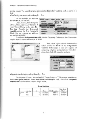
12. ChapterI GettingStarted
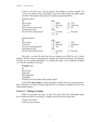
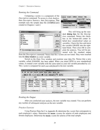
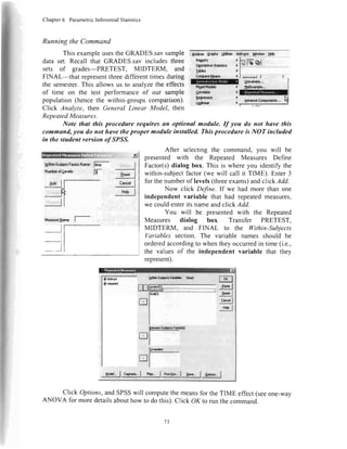
We want to compute the mean for the
variable called GRADE. Thus, we need to select
the variablename in the left window (by clicking
on it). To transferit to the right window, click on
the right arrow between the two windows. The
arrow always points to the window oppositethe
highlighted item and can be used to transfer
l:rt.Ij
in
m ;F* |
-t:g.J
-!tJ
PR:lf- Smdadr{rdvdarvai&
selectedvariablesin either direction.Note that double-clickingon the variablenamewill
also transfer the variable to the opposite window. StandardWindows conventionsof
"Shift" clickingor "Ctrl" clickingto selectmultiplevariablescanbe usedaswell.
When we click on the OK button,the analysiswill be conducted,and we will be
readyto examineour output.
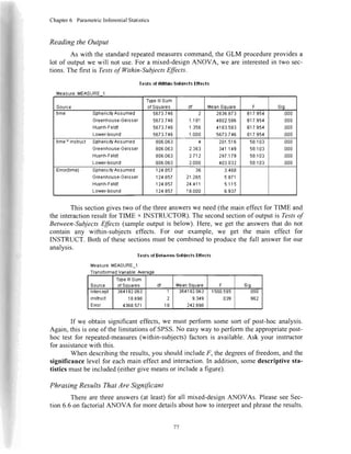
Section1.6 ExaminingandPrintingOutputFiles
After an analysis is performed, the output is
placedin the output window, and the output window
becomesthe active window. If this is the first analysis
you have conductedsince starting SPSS,then a new
output window will be created.If you haverun previous
outputisaddedto theendof yourpreviousoutput.
To switchbackandforthbetweenthedatawindowandtheoutput window,select
thedesiredwindowfromtheWindowmenubar(seearrow,below).
Theoutputwindowis splitintotwo sections.Theleftsectionis anoutlineof the
output(SPSSreferstothisasthe"outlineview").Therightsectionis theoutputitself.
irllliliirrillliirrrI -d
* lnl-Xj
H. Ee lbw A*t lra'dorm
-qg*g!r*!e!|ro_
Craphr,Ufr!3 Uhdo'N Udp
slsl*glelsl*letssJsl#_#rl+l*l +l-l&hjl :lqlel,
* Descrlptlves
f]aiagarll l: lrrs datcra&ple.lav
o
lle*crhlurr Sl.*liilca
N Mlnlmum Hadmum Xsrn Std.Dwiation
ufinuc
valldN(|lstrylsa)
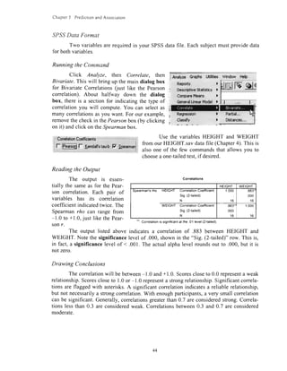
I
2
83.00 85.00 81,0000 1.41421
ffiffi?iffi rr---*.* r*4
The sectionon the left of the output window providesan outline of the entireout-
put window. All of the analysesarelistedin theorderin which they wereconducted.Note
that this outline can be usedto quickly locatea sectionof the output.Simply click on the
sectionyou would like to see,andtheright window will jump to the appropriateplace.
analysesandsavedthem,your
ornt
El Pccc**tvs*
r'fi Trb
6r**
lS Adi€D*ard
ffi Dcscrtfhcsdkdics

13. ChapterI GeningStarted
Clicking on a statisticalprocedurealsoselectsall of the outputfor thatcommand.
By pressingtheDeletekey,thatoutputcanbe deletedfrom the output window. This is a
quick way to be surethatthe output window containsonly the desiredoutput.Outputcan
also be selectedand pastedinto a word processorby clicking Edit, then Copy Objeclsto
copy the output.You canthenswitchto your word processorand click Edit, thenPaste.
To print your output,simply click File, thenPrint, or click on the printer icon on
the toolbar.You will havethe option of printing all of your outputor just the currentlyse-
lected section.Be careful when printing! Each time you mn a command,the output is
addedto the end of your previousoutput.Thus,you could be printing a very largeoutput
file containinginformationyou may not want or need.
Oneway to ensurethatyour output window containsonly the resultsof thecurrent
commandis to createa new output window just beforerunningthe command.To do this,
click File, thenNew, then Outpul. All your subsequentcommandswill go into your new
output window.
Practice Exercise
Load the sampledatafile you createdearlier(SAMPLE.sav).Run theDescriptives
commandfor the variableGRADE and print the output.Your output shouldlook like the
exampleon page7. Next,selectthedata window andprint it.
Section1.7 ModifyingDataFiles
Once you havecreateda datafile, it is really quite simple to add additionalcases
(rows/participants)or additionalvariables(columns).ConsiderExample1.7.1.
Example1.7.1
Twomorestudentsprovideyouwithsurveys.Theirinformationis:
ResponseSheet3
ID:
Dayof class:
Classtime:
Are you a morningperson?
Finalgradein class:
Do you work outsideschool?
ResponseSheet4
ID:
Day of class:
Classtime:
Are you a morningperson?
Finalgradein class:
Do you work outsideschool?
8734
80%
MWF
Morning
Yes
Full-time
No
1909
X MWF
X Morning
X Yes
73%
Full+ime
No
X TTh
Afternoon
XNo
Part-time
TTH
Afternoon
No
X Part-time

14. ChapterI GettingStarted
To addthesedata,simply placetwo additionalrows in theData View window (af-
ter loadingyour sampledata).Notice that asnew participantsareadded,the row numbers
becomebold. when done,the screenshouldlook like the screenshothere.
New variablescan also be added.For example,if the first two participantswere
given specialtrainingon time management,andthetwo new participantswerenot, thedata
file canbe changedto reflectthis additionalinformation.The new variablecould be called
TRAINING (whetheror not the participantreceivedtraining), and it would be codedso
that 0 : No and I : Yes. Thus,the first two participantswould be assigneda "1" andthe
Iasttwo participantsa "0." To do this, switch to the Variable View window, then add the
TRAINING variableto the bottom of the list. Then switchback to theData View window
to updatethe data.
f+rilf,t - tt Inl vl
Sa E& Uew Qpta lransform &rpFzc gaphs Lffitcs t/itFdd^,SE__--
14:TRAINING l0 lvGbt€ri of
t0 NAY TIME MORNING GRADE woRKI mruruwe 1r
1 4593.0f1 Tueffhu aterncon No 85.0u Nol Yes
I 1901.OCIManA/Ved/ m0rnrng Yes ffi.0n iiart?mel- yes
3 8734"00 Tueffhu momtng No 80.n0 Noi No
4 1909.00MonrlVed/ morning Yes 73.00 Part-TimeI No '
s
I
(l) .rView { Vari$c Vlew
. l-.1 =J "isPssW
rll'l
,i
Adding dataand addingvariablesarejust logical extensionsof the procedureswe
usedto originally createthe datafile. Savethis new data file. We will be using it again
laterin thebook.
'..,
j .l lrrl vl
nh E*__$*'_P$f_I'Sgr &1{1zcOmhr t$*ues$ilndonHug_
Tffiffi
ID DAY TIME MORNING GRADE WORK var ^
1 4593.00 Tueffhu aternoon No 85.00 No
2 1gnl.B0MonMed/ m0rnrng Yes 83.00 Part-Time
3 8734.00 Tue/Thu mornrng No 80,00 No
1909.00MonAfVed/ mornrng Yeg 73.00 Part-Time
)
.mfuUiewffi
I
rb$ Vbw / l{l rll
'.- - -,,,---Jd*
15P55Procus*rlsready I i ,4

15. ChapterI GettingStarted
Practice Exercise
Follow the exampleabove(whereTRAINING is the new variable).Make the
modificationsto yourSAMPLE.savdatafile andsaveit.
l0

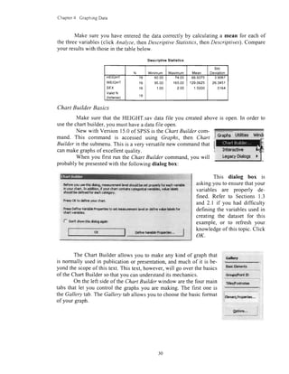
16. Chapter2
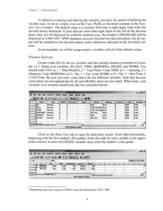
EnteringandModifying Data
In Chapter 1, we learnedhow to createa simpledatafile, saveit, perform a basic
analysis,and examinethe output.In this section,we will go into more detail aboutvari-
ablesanddata.
Section2.1 VariablesandDataRepresentation
In SPSS,variablesarerepresentedascolumnsin the datafile. Participantsarerep-
resentedasrows.Thus,if we collect4 piecesof informationfrom 100participants,we will
havea datafile with 4 columnsand 100rows.
Measurement Scales
Therearefour typesof measurementscales:nominal, ordinal, interval, andratio.
While themeasurementscalewill determinewhich statisticaltechniqueis appropriatefor a
given set of data,SPSSgenerallydoesnot discriminate.Thus, we startthis sectionwith
this warning: If you ask it to, SPSSmay conductan analysisthat is not appropriatefor
your data.For a morecompletedescriptionof thesefour measurementscales,consultyour
statisticstext or the glossaryin AppendixC.
Newer versionsof SPSSallow you to indicatewhich types of
data you have when you define your variable.You do this using the
Measurecolumn.You can indicateNominal,Ordinal,or Scale(SPSS
doesnot distinguishbetweeninterval andratio scales).
Look at the sampledatafile we createdin Chapterl. We calcu-
lateda mean for the variableGRADE. GRADE wasmeasuredon a ra-
tio scale,andthemeanis anacceptablesummarystatistic(assumingthatthedistribution
isnormal).
We could havehad SPSScalculatea mean for the variableTIME insteadof
GRADE.If wedid,wewouldgettheoutputpresentedhere.
TheoutputindicatesthattheaverageTIME was 1.25.RememberthatTIME was
coded as an ordinal variable (I =
morningclass,2-afternoon
class).Thus, the mean is not an
appropriatestatisticfor an ordinal
scale,but SPSScalculatedit any-
way. The importanceof consider-
ing the type of data cannot be
overemphasized. Just because
SPSSwill compute a statistic for
you doesnot meanthatyou should
Measure
@Nv
f $cale
.sriltr
r Nominal
ll
*lq]eH"N-ql*l trlllql eilr $l-g
:* Sl astts
.l.:D
gtb
:$sh
.6M6.ffi
$arlrba"t S#(|
ht6x0tMn a
LS 2.qg Lt@

17. ql total
2.00 2.Bn 4.00
3.00 1.00 4.00
4.00 3.00 7.00
2.00
1.00 2.UB 3.00
Chapter2 EnteringandModifying Data
useit. Later in the text,when specificstatisticalproceduresarediscussed,the conditions
underwhich they areappropriatewill be addressed.
Missing Data
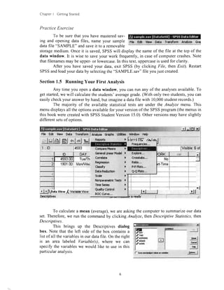
Often,participantsdo not providecompletedata.For somestudents,you may have
a pretestscorebut not a posttestscore.Perhapsone studentleft one questionblank on a
survey,or perhapsshedid not stateher age.Missing datacanweakenany analysis.Often,
a singlemissingquestioncaneliminatea sub-
ject from all analyses.
If you havemissingdatain your data
set, leave that cell blank. In the exampleto
the left, the fourth subjectdid not complete
Question2. Note thatthetotal score(which is
calculatedfrom both questions)is alsoblank
becauseof the missing data for Question2.
SPSSrepresentsmissing data in the data
window with a period(althoughyou should
not entera period-just leaveit blank).
Section2.2 TransformationandSelectionof Data
Weoftenhavemoredatain a datafile thanwewantto includein a specificanaly-
sis.For example,our sampledatafile containsdatafrom four participants,two of whom
receivedspecialtrainingandtwo of whomdid not.If we wantedto conductananalysis
usingonlythetwo participantswhodidnotreceivethetraining,we wouldneedto specify
theappropriatesubset.
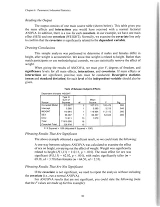
Selectinga Subset
F|! Ed vl6{ , O*. lr{lrfum An*/& e+hr (
We canusethe SelectCasescommandto specify
a subset of our data. The Select Cases command is
located under the Data menu. When you select this
command,the dialog box below will appear.
t'llitl&JE
il :id
O*fFV{ldrr PrS!tU6.,.
CoptO.tafropc,tir3,..
l,j.l,/r,:irrlrr! lif l ll:L*s,,.
Hh.o*rr,.,
Dsfti fi*blc Rc*pon$5ct5,,,
ConyD*S
sd.rt Csat
You can specify which cases(partici-
pants)you want to selectby using the selec-
tion criteria,which appearon the right sideof
theSelectCasesdialogbox.
q*d-:-"-- "-"""-*--*--**-""*-^*l
6 Alce
a llgdinlctidod
,rl
r irCmu*dcaa ]
i*np* | i{^ lccdotincoarrpr
:
;.,* |
-:--J
c llaffrvci*lc
l0&t
C6ttSldrDonoan!.ffi
foKl aar I c-"rl x* |
t2

18. Chapter2 EnteringandModifying Data
By default,All caseswill be selected.The most commonway to selecta subsetis
to click If condition is satisfied,thenclick on the button labeledfi This will bring up a
newdialogbox thatallowsyou to indicatewhichcasesyou would like to use.
You can enter the logic
used to select the subsetin the
upper section. If the logical
statement is true for a given
case, then that case will be
selected.If the logical statement
is false. that case will not be
selected.For example, you can
selectall casesthat were coded
as Mon/Wed/Fri by enteringthe
formula DAY = I in the upper-
?Ais"I c'-t I Ht I
rightpartof thewindow.If DAY is l, thenthestatementwill betrue,andSPSSwill select
the case.If DAY is anythingotherthan l, the statementwill be false,andthe casewill not
be selected.Once you have enteredthe logical statement,click Continueto return to the
SelectCasesdialogbox. Then,click OK to returnto thedata window.
After you haveselectedthecases,thedata window will changeslightly.
The casesthat werenot selectedwill be markedwith a diagonalline throughthe
casenumber.For example,for our sampledata,the first and third casesarenot
selected.only the secondandfourthcasesareselectedfor this subset.
U;J;J:.1-glL1 E{''di',*tI
, 'J-e.l-,'JlJ.!J-El[aasi"-Eo,t----i
ilqex4q lffiIl,?,l*;*"'=
,Jl _!JlJ 0 U IAFTAN(r"nasl
sl"J=tx-s*t"lBi!?Blt1trb:r
1
I
,
I
I
l
i{
1
,1
'l
1
I
1
:
t
'l
1
'l
EffEN'EEEgl''EEE'o ,.,:r. rt lnl vl
!k_l**
-#gdd.i.&lFlib'-
ID TIME MORNING ERADE WORK TRAINING
/,-< 4533.m Tueffhui affsrnoon No ffi.m Na Yes NotSelected
2 1901.m-
6h4lto*-
ieifrfft
MpnMed/i mornino. -..- ^,-.-.*.*..,-- J.- . - .-..,..".*-....- ':
Yss 83,U1Fad-Jime Yes Splacled
-'4
TuElThu. morning No m.m No No NotSelected
4 MonA/Ved/1morning Yes ru.mPart-Time No
s
!LJii. vbryJv,itayss7 I . *-J *]fsPssProcaesaFrcady I i ,1,
An additionalvariablewill also be createdin your data file. The new variableis
calledFILTER_$ andindicateswhethera casewasselectedor not.
If we calculatea mean
GRADE using the subsetwe
just selected,we will receive
the output at right. Notice that
we now havea mean of 78.00
with a samplesize(M) of 2 in-
steadof 4.
DescripthreStailstics
N Minimum Maximum Mean
std.
Deviation
UKAUE
ValidN
IliclwisP'l
2
2
73.00 83.00 78.0000 7.0711
l3

19. Chapter2 EnteringandModifyingData
Be carefulwhen you selectsubsets.Thesubsetremainsin ffict until you run the
commandagain and selectall cases.You cantell if you havea subsetselectedbecausethe
bottomof the data window will indicatethat a filter is on. In addition,when you examine
your output,N will be lessthanthe total numberof recordsin your dataset if a subsetis
selected.The diagonallines throughsomecaseswill also be evidentwhen a subsetis se-
lected.Be carefulnot to saveyour datafile with a subsetselected,asthis cancauseconsid-
erableconfusionlater.
Computing a New Variable
SPSScan alsobe used
to computea new variable or
manipulateyour existing vari-
ables. To illustrate this, we
will create a new data file.
This file will contain data for
four participants and three
variables(Ql, Q2, and Q3).
The variables represent the
number of points each
participant received on three
different questions.Now enter
the data shown on the screen to the right. When done, save this data file as
"QUESTIONS.sav."We will beusingit againin laterchapters.
I TrnnsformAnalyze Graphs Utilities Whds
Rersdeinto5ameVariable*,,,
RacodointoDffferantVarlables.,,
Ar*omSicRarode,,.
Vlsual8inrfrg,..
After clicking the Compute Variable
command,we get the dialog box at
right.
The blank field marked Target
Variable is where we enter the name
of the new variablewe want to create.
In this example, we are creating a
variablecalled TOTAL, so type the
word"total."
Notice that there is an equals
sign between the Target Variable
blank and the Numeric Expression
blank. Thesetwo blank areasare the
Now you will calculatethe total scorefor
eachsubject.We coulddo this manually,but if the
data file were large, or if there were a lot of
questions,this would take a long time. It is more
efficient (and more accurate) to have SPSS
compute the totals for you. To do this, click
Transform and then click Compute Variable.
U $J-:iidijl
lij -!CJ:l Jslcl
ll;s rtg-sJ
rt rt rl ,_g-.|J
:3 lll--g'L'"J til
, rr | {q*orfmsrccucrsdqf
l4
nh E* vir$, D.tr T|{dorm
*lslel EJ-rlrj -lgltj{l -|tlf,la*intt m eltj I
l* ,---- LHJ
{#i#ffirtr!;errtt*;
,
rrwI i+t*...
*l
gl
w
ca
lllmr*dCof
0rr/ti*
&fntndi)
Oldio.
E${t iil
:J
n*ri c*rl
"*l

20. Chapter2 EnteringandModifying Data
iii:Hffiliji:.:
.i .i>t ii"alCt
i-Jr:J::i i-3J:J
l:j -:15 JJJI
tJ -tJ-il --q-|J
is:Jlll --q*J m
|f-- | ldindm.!&dioncqdinl
tsil nact I c:nt I x* |
two sides of an equation that SPSS
will calculate.For example,total: ql
+ q2 + q3 is the equationthat is
enteredin the samplepresentedhere
(screenshotat left).Notethatit is pos-
sible to create any equation here
simply by using the number and
operationalkeypad at the bottom of
the dialog box. When we click OK,
SPSSwill createa new variablecalled
TOTAL andmakeit equalto the sum
of thethreequestions.
Save your data file again so
thatthenew variablewill be available
for futuresessions.
-lJ
t::,, - ltrl-Xl
Sindow Help
3.n0 3.0n 4,n0 10.00
4.00
31 2.ool 2.oo..........;.
41 1.001 3001
.:1 l-'r--i-----i
I il I i
, l, lqg,t_y!"*_i VariabteViewJ lit rljl
W*;
Recodinga Variable-Dffirent Variable
SPSS can create a new
variable based upon data from
another variable. Say we want to
split our participantson the basisof
their total score.We want to create
a variablecalledGROUP,which is
coded I if the total score is low
(lessthanor equalto 8) or 2 if the
total scoreis high (9 or larger).To
do this, we click Transform, then
Recodeinto Dffirent Variables.
,-.lu l,rll r-al +. conp$ovdiouc','
---.:1.- Cd.nVail'r*dnCasas.,,
l{
-l
I -- -
rr 'rtr I o..**^c--u-r-c
4.00
2.00
i.m
Racodrlrto 0ffrror* Yal
Art(tn*Rrcodr...
U*dFhn|ro,,.
S*a *rd llm tllhsd,,,
Oc!t6 I}F sairs..,
Rid&c l4sitE V*s.,.
Rrdon iMbar G.rs*trr,,.
l5
Eile gdit SEw Qata lransform $nalyza 9aphs [tilities Add'gns
F{| [dt !la{ Data j Trrx&tm Analrra

21. Chapter2 EnteringandModifyingData
This will bring up the
Recode into Different Variables
dialog box shown here. Transfer
the variableTOTAL to the middle
blank. Type "group" in the Name
field underOutputVariable.Click
Change,and the middle blank will
show that TOTAL is becoming
GROUP.asshownbelow.
ladtnl c€ rlccdm confbil
-'tt"
I rygJ**l-H+ |
r t *.!*lr
r&*ri*i*t
;rln
I r-":-'-'1**
lirli
iT-
I r nryrOr:frr**"L
,f-
i c nq.,saa*ld6lefl;
F-
,.F--*-_-_-_____
: "
*r***o
I a lrt*cn*r
I I nni.
rT..".''..."...-
I ir:L-_-
t'
l6 i4i'|(tthah*
;F-
I"
n*'L,*l'||.r.$,
: r----**-:
;
r {:ei.*
T &lrYdd.r*t li--
'-
i"r,.!*r h^.,",r y..,t larir,r it:.' I
gf-ll $q I
'*J
til
To help keep track of variablesthat have
been recoded, it's a good idea to open the
Variable View and enter"Recoded"in the Label
column in the TOTAL row. This is especially
useful with large datasetswhich may include
manyrecodedvariables.
Click Old andNew Values.This will bring
up the Recodedialog box. In this example,we
have entered a 9 in the Range, value through
HIGHEST field and a 2 in the Value field under
New Value.When we click Add, theblank on the
right displaysthe recodingformula.Now enteran
8 on the left in the Range, LOWEST through
valueblank and a I in the Valuefield underNew
Value.Click Add, thenContinue.Click OK. You
will be redirectedto the data window. A new
variable (GROUP) will have been added and
codedas I or 2, basedon TOTAL.
*u"'." -ltrlIl
Flc Ed Yl.ly Drt! Tr{lform {*!c ce|6.,||tf^,!!!ry I+
NtnHbvli|bL-lo|rnrV*#r
l6

22. Chapter3
DescriptiveStatistics
ln Chapter2, wediscussedmanyof theoptionsavailablein SPSSfor dealingwith
data.Now we will discusswaysto summarizeour data.Theproceduresusedto describe
andsummarizedataarecalleddescriptivestatistics.
Section3.1 FrequencyDistributionsand PercentileRanks
for a SingleVariable
Description
TheFrequenciescommandproducesfrequencydistributionsfor thespecifiedvari-
ables.Theoutputincludesthenumberof occurrences,percentages,validpercentages,and
cumulativepercentages.Thevalid percentagesandthe cumulativepercentagescomprise
onlythedatathatarenotdesignatedasmissing.
TheFrequenciescommandis usefulfor describingsampleswherethemeanis not
useful(e.g.,nominalor ordinalscales).It is alsousefulasa methodof gettingthefeelof
yourdata.It providesmoreinformationthanjust a meanandstandarddeviationandcan
beusefulin determiningskewandidentifyingoutliers.A specialfeatureof thecommand
isitsabilityto determinepercentileranks.
Assumptions
Cumulativepercentagesandpercentilesarevalidonly for datathataremeasured
onat leastanordinal scale.Becausetheoutputcontainsonelinefor eachvalueof a vari-
able,thiscommandworksbestonvariableswitharelativelysmallnumberof values.
Drawing Conclusions
TheFrequenciescommandproducesoutputthatindicatesboththenumberof cases
in thesampleof a particularvalueandthepercentageof caseswith thatvalue.Thus,con-
clusionsdrawnshouldrelateonlyto describingthenumbersor percentagesof casesin the
sample.If thedataareatleastordinalin nature,conclusionsregardingthecumulativeper-
centageand/orpercentilescanbedrawn.
.SPSSData Format
TheSPSSdatafile for obtainingfrequencydistributionsrequiresonlyonevariable,
andthatvariablecanbeof anytype.
tt

23. Chapter3 DescriptiveStatistics
Creating a Frequency Distribution
To run the Frequer?ciescommand,
click Analyze, then Descriptive Statistics,
then Frequencies.(This exampleusesthe
CARS.savdatafile that comeswith SPSS.
It is typically located at <C:Program
FilesSPSSCars.sav>.)
This will bring up the main dialog
box. Transferthe variablefor which you
would like a frequencydistributioninto the
Disbtlvlr...
N
Erpbr,..
croac*a,..
Rrno,.,
F.Pt'lok,.,
aaPUs,.,
Variable(s)blank to the right. Be surethat
the Display frequency tables option is
checked.Click OK to receiveyour output.
Note that the dialog boxes in
newer versionsof SPSSshow both the
typeof variable(theicon immediatelyleft
of the variable name) and the variable
labels if they are entered. Thus, the
variableYEAR shows up in the dialog
box asModel Year(moduloI0).
i:rl.&{l&l&lslsl}sl
i1 rmpg i18
MilesperGallonlmr
/Erqlr,onispUcamr
/ Hurepowor[horc
dv*,id"w"bir 1|ut
d t!rc toAceileistc
dr',Ccxr*yolOrbin[c
l7 Oisgayhequercytder
xl
q!l
jq? |
.f"tq I
. He_l
sr**i,1..1f*:.,.I rry*,:.I
Outputfor a Frequency Distribution
The outputconsistsof two sections.The first sectionindicatesthe numberof re-
cordswith valid data for eachvariableselected.Recordswith a blank scorearelistedas
missing.In thisexample,thedatafile contained406 records.Noticethatthevariablelabel
is ModelYear(modulo100).
statistics
The second section of the output contains a
cumulative frequency distribution for each variable
Wselected.Atthetopofthesection,thevariablelabelis
|
* y.1"1 |
oo?
| given.The outputiiself consistsof five columns.The first
I MissingI t I Jolumnliststhi valuesof thevariablein sortedorder.There
is a row for eachvalueof your variable,
and additionalrows are added at the
bottom for the Total and Missing data.
The secondcolumngivesthe frequency
of eachvalue,includingmissingvalues.
Thethirdcolumngivesthepercentageof
all records (including records with
missingdata)for eachvalue.The fourth
column,labeledValidPercenl,givesthe
percentageof records(withoutincluding
records with missing data) for each
value.If therewereany missingvalues,
thesevalueswould be larger than the
valuesin columnthreebecausethe total
ModolYo.r (modulo 100)
Pcrcenl Valid P6rc€nl
Cumulativs
vatE
72
73
74
75
76
77
79
80
81
82
Total
Missing 0 (Missing)
Total
34
28
40
27
30
34
28
29
29
30
31
405
1
406
I 4
7.1
6.9
9.9
6.7
8.4
6.9
8.9
7.1
7.1
7.4
7.6
99.8
100.0
I 4
7.2
6.9
9.9
6.7
7.4
8.4
6.9
8.9
f.2
7.2
7.4
7.7
100.0
E4
15.6
22.5
32.3
39.0
46.4
54.8
61.7
70.6
77.8
84.9
92.3
|00.0
r8
&99rv I
@
cdrFrb'l{tirE }
r5117gl

24. Chapter3 DescriptiveStatistics
numberof recordswould havebeenreducedby thenumberof recordswith missingvalues.
The final column gives cumulativepercentages.Cumulativepercentagesindicatethe per-
centageof recordswith a scoreequalto or smallerthan the currentvalue.Thus, the last
value is always 100%.Thesevaluesare equivalentto percentile ranks for the values
listed.
Determining PercentiIe Ranl<s
:,,.
tril
YI
!rydI
|*"1
lT Oirpbarfrcqlcreyttblce
frfix*... I
Central TendencyandDispersior sections
suchasthe Median or Mode. whichcannot
(seeSection3.3).
This brings up the Frequencies:
Statisticsdialog box. Check any additional
desiredstatisticby clickingon the blanknext
to it. For percentiles, enter the desired
percentile rank in the blank to the right of
thePercentile(s)label.Then,click Add to add
it to the list of percentilesrequested.Once
you haveselectedall your requiredstatistics,
click Continue to return to the main dialog
box.Click OK.
The Frequencies command can be
used to provide a number of descriptive
statistics,as well as a variety of percentile
values(includingquartiles, cut points,and
scorescorrespondingto a specificpercentile
rank).
To obtain either the descriptiveor
percentile functions of the Frequencies
command,click the Statisticsbutton at the
bottomof the maindialog box. Note thatthe
of this box are useful for calculatingvalues,
be calculatedwith theDescriptiyescommand
PscdibV.lrr
xl
c{q I
*g"d I
Hdo I
tr Ourilr3
I
F nrs**rtd!i* ,crnqo,p, i
f- Vdrixtgor0mi&ohlr
Oi$.r$pn"
l* SUaa**
n v$*$i
I* nmgc
f Mi*n n
|- Hrrdilrtl
l- S"E.mcur
0idthfim'
t- ghsrurt
T Kutd*b
Statistics
ModelYear(modulo100
N Vatid
Missing
Percentiles 25
50
75
80
405
1
73.00
76.00
79.00
80.00
Outputfor PercentileRanl<s
The Statisticsdialog box adds on to the
previousoutput from the Frequenciescommand.The
new sectionof theoutputis shownat left.
The output containsa row for eachpieceof
informationyou requested.In the exampleabove,we
checkedQuartilesand askedfor the 80th percentile.
Thus, the output contains rows for the 25th, 50th.
75th,and80thpercentiles.
Mla pa Galmlm3
Sfndr*Pi*rcsnr
SHslsp{rierltuso
/v***v*$t*(ttu
/lino toaccrbrar
$1C**{ry o{Origr[c
l9

25. Chaprer,1 Descriptire Statistics
PracticeExercise
UsingPracticeDataSetI in AppendixB, createa frequencydistributiontablefor
themathematicsskillsscores.Determinethemathematicsskillsscoreat whichthe60th
percentilelies.
section3.2 FrequencyDistributionsand percentileRanks
for Multiple Variables
Description
The Crosslabscommandproducesfrequencydistributionsfor multiplevariables.
Theoutputincludesthenumberof occurrencesof eachcombinationof levelJof eachvari-
able.It ispossibleto havethecommandgivepercentagesfor anyor all variables.
The Crosslabscommandis usefulfor describingsampleswherethe meanis not
useful(e'g.,nominalor ordinalscales).It is alsousefulasa methodfor gettinga feelfor
yourdata.
Assumptions
Becausethe outputcontainsa row or columnfor eachvalueof a variable.this
commandworksbestonvariableswitharelativelysmallnumberof values.
ThisexampleusestheSAMpLE.savdata ;ilffi;
file, which you createdin Chapter l. To run the chrfy
procedure, ctick Analyze, then Descriptive DttaRcd.Etbn
Statistics,then Crosstabs.This will bring up ttt.
scah
mainCrosstabsdialogbox,below.
,SPSSData Format
The SPSSdata file for the Crosstabs
commandrequirestwo or morevariables.Those
variablescanbeof anytype.
RunningtheCrosstabsCommand
I lnalyzc Orphn Ut||Uot
RcF*r )
(orprycrllcEnr
G*ncralllrgarFlodcl
The dialog box initially lists all vari-
ableson the left and containstwo blanks la-
beled Row(s) and Column(s). Enter one vari-
able(TRAINING) in theRow(s)box. Enterthe
second (WORK) in the Column(s) box. To
analyzemore than two variables,you would
enter the third, fourth, etc., in the unlabeled
area(ust undertheLayer indicator).
)
)
,
)
)
)
)
i,
Ror{.} T€K I
r---r ftr;;ho.- '-l
lrJ I
.;lm&! ryq I
20

26. Chapter3 DescriptiveStatistics
percentagesand other information to be generatedfor
eachcombinationof values.Click Cells,andyou will get
thebox at right.
For the example presentedhere, check Row,
Column, and Total percentages.Then click Continue.
This will return you to the Crosstabsdialog box. Click
OK to run theanalvsis.
TRAINING'WURKCross|nl)tilntlo|l
WORK
TolalNO Parl-Time
TRAINING Yes Count
%withinTRAININO
%withinwoRK
%ofTolal
I
50.0%
50.0%
25.0%
1
50.0%
50.0%
25.0%
100.0%
50.0%
50.0%
No Count
%withinTRAINING
%withinWORK
%ofTolal
1
50.0%
50.0%
25.0%
1
50.0%
50.0%
25.0%
?
1000%
50.0%
50.0%
Total Count
%withinTRA|NtNo
%wilhinWORK
%ofTolal
50.0%
100.0%
50.0%
a
500%
100.0%
50.0%
4
r00.0%
100.0%
100.0%
Interpreting Crosstabs Output
The output consistsof a
contingencytable.Each level of
WORK is given a column.Each
level of TRAINING is given a
row. In addition, a row is added
for total, and a column is added
for total.
The Cells button allows you to specify W:
t C",ti* |
t*"1
,"1
Eachcell containsthe numberof participants(e.g.,one participantreceivedno
traininganddoesnot work; two participantsreceivedno training,regardlessof employ-
mentstatus).
Thepercentagesfor eachcell arealsoshown.Row percentagesaddup to 100%
horizontally.Columnpercentagesaddupto 100%vertically.Forexample,of all theindi-
vidualswhohadno training, 50ohdid notworkand50o%workedpart-time(usingthe"o/o
withinTRAINING" row).Of theindividualswhodid notwork,50o/ohadno trainingand
50%hadtraining(usingthe"o/owithinwork"row).
Practice Exercise
UsingPracticeDataSet I in AppendixB, createa contingencytableusingthe
Crosstabscommand.Determinethe numberof participantsin eachcombinationof the
variablesSEXandMARITAL. Whatpercentageof participantsis married?Whatpercent-
ageof participantsis maleandmarried?
Section3.3 Measuresof Central Tendencyand Measuresof Dispersion
for a SingleGroup
Description
Measuresof centraltendencyarevaluesthat representa typicalmemberof the
sampleor population.Thethreeprimarytypesarethemean,median,andmode.Measures
of dispersiontell you thevariabilityof yourscores.Theprimarytypesaretherangeand
thestandarddeviation.Together,a measureof centraltendencyanda measureof disper-
sionprovideagreatdealof informationabouttheentiredataset.
''Pd€rl.!p. - r-Bait*"
;F Bu : ,l- U]dadr&ad
F corm if- sragatrd
"1'"1--_rry-ys___ .
2l

27. Chapter,l DescriptiveStatistics
We will discussthesemeasuresof central
tendencyandmeasuresof dispersionin the con-
text of the Descriplives command. Note that
many of thesestatisticscan also be calculated
with several other commands (e.g., the
Frequenciesor CompareMeans commandsare
requiredto computethe mode or median-the
Statisticsoption for theFrequenciescommandis
shownhere).
iffi{ltl*::l'.,xl
Fac*Vd*c-----:":'-'-"-" "-
|7 Arruer
|* O*pai*furjF tqLteiotpr
F rac$*['*
r.-I 16-k'I
':'I I+l
lcer**r**nc*r1 !*{* |
f- rlm Cr* |
, f u"g.t -:.-i
i0hx*ioo*".'*-'
lf Sld.dr',iitbnl* lli*nn
]fV"iro
f.H**ntrn
lfnxrgo f.5.t.ncr
: T Modt
:-^t5m
l- Vdsm$apn&bcirr
oidrlatin-- --
r5tcffi:
; f Kutu{b
i
Assumptions
Eachmeasureof centraltendencyandmeasureof dispersionhasdifferent assump-
tionsassociatedwith it. The mean is the mostpowerfulmeasureof centraltendency,andit
hasthe mostassumptions.For example,to calculatea mean,the datamustbe measuredon
an interval or ratio scale.In addition,thedistributionshouldbe normally distributedor, at
least,not highly skewed.The median requiresat leastordinal data.Becausethe median
indicatesonly the middle score(when scoresarearrangedin order),thereareno assump-
tions aboutthe shapeof the distribution.The mode is the weakestmeasureof centralten-
dency.Thereareno assumptionsfor the mode.
The standard deviation is themostpowerful measureof dispersion,but it, too, has
severalrequirements.It is a mathematicaltransformationof the variance (the standard
deviationis the squareroot of thevariance).Thus,if oneis appropriate,theotheris also.
The standard deviation requiresdatameasuredon an interval or ratio scale.In addition,
the distributionshouldbe normal.The range is the weakestmeasureof dispersion.To cal-
culatea range, the variablemustbe at leastordinal. For nominal scaledata,the entire
frequencydistributionshouldbe presentedasa measureof dispersion.
Drawing Conclusions
A measureof centraltendencyshouldbe accompaniedby a measureof dispersion,
Thus, when reporting a mean, you shouldalso report a standard deviation. When pre-
sentinga median, you shouldalsostatetherange or interquartilerange.
.SPSSData Format
Only onevariableis required.
22

28. Chapter3 DescriptiveStatistics
Running the Command
The Descriptives command will be the
command you will most likely use for obtaining
measuresof centraltendencyandmeasuresof disper-
sion. This exampleusesthe SAMPLE.sav data file
we haveusedin thepreviouschapters.
,t X
dlt
da.v
qil
n".dI
cr*l I
f,"PI
opdqr"..I
To run the command, click Analyze,
then Descriptive Statistics,then Descriptives.
This will bring up the main dialog box for the
Descriptives command. Any variables you
would like informationaboutcanbe placedin
the right blank by double-clickingthem or by
selectingthem,thenclicking on theanow.
!
D
' cond*s
. Rolrar*n
: classfy
: 0€tdRedrctitrt
)
)
)
)
d**
?n-"*
?,r,qx
/t**ts
f S&r dr.d!r&!d Y*rcr ri vdi.bb
By default, you will receivethe N (number of
cases/participants),the minimum value, the maximum
value,the mean, and the standard deviation.Note that
someof thesemay not be appropriatefor the type of data
you haveselected.
If you would like to changethe defaultstatistics
that aregiven, click Optionsin the main dialog box. You
will begiventheOptionsdialogbox presentedhere.
F Morr l- Slm r@t
qq..'I
,|'?bl
ltl
{l
'!t
,l
,lt
il
'i
I
I
:
"i
I
",
;i
I
;
F su aa**n F, Mi*ilm
f u"or- F7Maiilrn
l- nrrcr I- S.r.npur
I otlnyotdq: *
I {f V;i*hlC
I r lpr,*an
I
r *car*remar
i r Dccemdnnmre
Reading the Output
The output for the Descriptivescommandis quite straightforward.Each type of
outputrequestedis presentedin a column,andeachvariableis given in a row. The output
presentedhereis for the sampledatafile. It showsthatwe haveonevariable(GRADE) and
that we obtainedthe N, minimum, maximum,mean, and standard deviation for this
variable.
DescriptiveStatistics
N Minimum Maximum Mean Std.Deviation
graoe
ValidN (listwise)
4
4
73.00 85.00 80.2500 5.25198
lA-dy* ct.dn Ltffibc
GonardtFra*!@
23

29. Chapter3 DescriptiveStatistics
Practice Exercise
UsingPracticeDataSet I in AppendixB, obtainthe descriptivestatisticsfor the
ageof theparticipants.What is themean?The median?The mode?What is thestandard
deviation?Minimum?Maximum?The range?
Section3.4 Measuresof Central Tendency and Measuresof Dispersion
for Multiple Groups
Description
The measuresof centraltendencydiscussedearlierare often needednot only for
theentiredataset,but alsofor severalsubsets.Oneway to obtainthesevaluesfor subsets
would be to usethe data-selectiontechniquesdiscussedin Chapter2 andapply theDe-
scriptivescommandto eachsubset.An easierway to performthis task is to usetheMeans
command.The Meanscommandis designedto providedescriptivestatisticsfor subsets
ofyour data.
Assumptions
The assumptionsdiscussedin the sectionon Measuresof CentralTendencyand
Measuresof Dispersionfor a SingleGroup(Section3.3)alsoapplyto multiplegroups.
Drawing Conclusions
A measureof centraltendencyshouldbe accompaniedby a measureof dispersion.
Thus,whengiving a mean,you shouldalsoreporta standarddeviation.Whenpresenting
a median,you shouldalsostatetherangeor interquartilerange.
SPSSData Format
Two variablesin the SPSSdatafile are required.One representsthe dependent
variable and will be the variablefor which you receivethe descriptivestatistics.The
otheris theindependentvariable andwill beusedin creatingthesubsets.Notethatwhile
SPSScallsthis variablean independentvariable, it may not meetthe strictcriteriathat
definea trueindependentvariable (e.g.,treatmentmanipulation).Thus,someSPSSpro-
ceduresreferto it asthegroupingvariable.
RunningtheCommand
This example ! RnalyzeGraphsUtilities
nsportt F
' DescriptiveStatistirs )
GeneralLinearftladel F
' Csrrelata )
. Regression I
' (fassify F
WindowHetp I-l
r.l
Firulbgt5il |
-
Ona-Sarnplef feft.
Independent-SamdesTTe
Falred-SarnplEsTTest,,,
Ons-Way*|iJOVA,,,
uses the
SAMPLE.sav data file you created in
Chapterl. The Meanscommandis run by
clicking Analyze, then Compare Means,
thenMeans.
This will bringup the maindialog
box for the Means command. Place the
selectedvariablein the blank field labeled
DependentList.
1A
LA

30. Chapter3 DescriptiveStatistics
Placethe grouping variable in thebox labeledIndependentList.In this example,
throughuseof the SAMPLE.savdatafile, measuresof centraltendencyand measuresof
dispersion for the variable GRADE will be given for each level of the variable
MORNING.
:I
tu
DependantList
€ arv
,du**
/wqrk
€tr"ining
rTril
ll".i I
lLayarlal1*-
I :'r:rrt| ..!'l?It.Ii
I IndependentLi$:
i r:ffi
lr-, tffi,
r l*i.rl I
L-:-
ryl
HesetI
CancelI
l"rpI
By default,the mean,numberof cases,and
standard deviation are given. If you would like
additionalmeasures,click Optionsand you will be
presentedwith the dialog box at right. You can opt
to includeany numberof measures.
Reading the Output
The output for the Means commandis split
into two sections.The first section,called a case
processingsummary, gives informationaboutthe
data used. In our sample data file, there are four
students(cases),all of whom were includedin the
analysis.
I
Std.Enord Kutosis
Skemrcro
fd Stdirtlx:
mil'*-*
lltlur$uofCa*o*
lStardad
Doviaion
ml
I
I
Lqlry-l c""dI x,r I
Sld.Enool$karm
HanorricMcan :J
Medan
5tt
Minirn"rm
Manimlrn
Rarqo
Fist
La{
VsianNc
GaseProcessingSummary
Cases
lncluded Excluded Total
N Percent N Percent N Percent
grade- morning 4 100.0% 0 .OYo 4 | 100.0%
25

31. Chapter3 DescriptiveStatistics
The secondsectionof the out-
put is the report from the Means com-
mand.
This report lists the name of
the dependent variable at the top
(GRADE). Every level of the inde-
pendent variable (MORNING) is
shown in a row in the table.In this example,the levelsare 0 and l, labeledNo and Yes.
Note thatif a variableis labeled,thelabelswill be usedinsteadof theraw values.
The summarystatisticsgiven in the reportcorrespondto the data,wherethe level
of theindependentvariable is equalto therow heading(e.g.,No, Yes).Thus,two partici-
pantswereincludedin eachrow.
An additionalrow is added,namedTotal. That row containsthe combineddata.
andthe valuesarethe sameasthey would be if we hadrun theDescriptiyescommandfor
thevariableGRADE.
Extension to More Than One Independent Variable
If you have more than one
independent variable, SPSScan
break down the output even fur-
ther. Rather than adding more
variables to the Independent List
section of the dialog box, you
need to add them in a different
layer. Note that SPSS indicates
with which layeryou areworking.
If you click Next, you will be presentedwith
Layer 2 of 2, and you can selecta secondindependent
variable (e.g., TRAINING). Now, when you run the
command(by clicking On, you will be given summary
statistics for the variable GRADE by each level of
MORNING andTRAINING.
Your output will look like
the output at right. You now have
two main sections(No and yes),
along with the Total. Now, how-
ever, each main section is broken
down into subsections(No, yes,
andTotal).
The variable you used in
Level I (MORNING) is the first
one listed,and it definesthe main
sections.The variableyou had in
Level 2 (TRAINING) is listedsec-
Repott
GRADE
MORNING Mean N Std.Deviation
NO
Yes
Total
82.5000
78.0000
80.2500
2
4
3.53553
7.07107
5.25198
Report
ORADE
MORNING TRAINING Mean N Std.Deviation
No Yes
NO
Total
85.0000
80.0000
82.5000
1
1
I 3.53553
Yes Yes
NO
Total
83.0000
73.0000
78.0000
1
1
1
7.07107
Total Yes
NO
Total
84.0000
76.5000
80.2500
a
z
4
1.41421
4.54575
5.?5198
id
26

32. Chapter3 DescriptiveStatistics
ond.Thus,the first row representsthoseparticipantswho werenot morningpeopleand
whoreceivedtraining.Thesecondrowrepresentsparticipantswhowerenotmorningpeo-
pleanddid notreceivetraining.Thethirdrow representsthetotalfor all participantswho
werenotmorningpeople.
Noticethatstandarddeviationsarenotgivenfor all of therows.Thisis because
thereisonlyoneparticipantpercellin thisexample.Oneproblemwithusingmanysubsets
is thatit increasesthenumberof participantsrequiredto obtainmeaningfulresults.Seea
researchdesigntextor yourinstructorfor moredetails.
Practice Exercise
UsingPracticeDataSetI in AppendixB, computethemeanandstandarddevia-
tion of agesfor eachvalueof maritalstatus.Whatis theaverageageof themarriedpar-
ticipants?Thesingleparticipants?Thedivorcedparticipants?
Section3.5 Standard Scores
Description
Standardscoresallowthecomparisonof differentscalesby transformingthescores
intoa commonscale.Themostcommonstandardscoreis thez-score.A z-scoreis based
ona standardnormaldistribution(e.g.,a meanof 0 anda standarddeviationof l). A
z-score,therefore,representsthenumberof standarddeviationsaboveor belowthemean
(e.9.,az-scoreof -1.5representsascoreI %standarddeviationsbelowthemean).
Assumptions
Z-scoresarebasedon thestandardnormal distribution.Therefore,thedistribu-
tionsthatareconvertedtoz-scoresshouldbenormallydistributed,andthescalesshouldbe
eitherintervalor ratio.
Drawing Conclusions
Conclusionsbasedonz-scoresconsistof thenumberof standarddeviationsabove
or belowthemean.Forexample,astudentscores85onamathematicsexamin aclassthat
hasa meanof 70andstandarddeviationof 5.Thestudent'stestscoreis l5 pointsabove
theclassmean(85- 70: l5). Thestudent'sz-scoreis 3 becauseshescored3 standard
deviationsabovethemean(15+ 5 :3). If thesamestudentscores90ona readingexam,
witha classmeanof 80anda standarddeviationof 10,thez-scorewill be I .0because
sheis onestandarddeviationabovethe mean.Thus,eventhoughher raw scorewas
higheronthereadingtest,sheactuallydidbetterin relationto otherstudentsonthemathe-
maticstestbecauseherz-scorewashigheronthattest.
.SPSSData Format
Calculatingz-scoresrequiresonlya singlevariablein SPSS.Thatvariablemustbe
numerical.
27

33. Chapter3 DescriptiveStatistics
Running the Command
Computingz-scoresis a componentof the
Descriptivescommand.To accessit, click Analyze,
thenDescriptive Statistics,thenDescriptives. This
exampleusesthe sampledata file (SAMPLE.sav)
createdin ChaptersI and2.
19 Srva*ndudi3advduosts vcriaHas
Myzc eqhs Uti$tbl WMow Help
) b,lrstlK- al
@nerdLlneuFbdel )
Correlate )
This will bring up the stan-
dard dialog box for the Descrip-
/ives command.Notice the check-
box in the bottom-left corner la-
beled Save standardized values as
variables.Checkthis box andmove
the variableGRADE into the right-
handblank. Then click OK to com-
pletethe analysis.You will be pre-
sented with the standard output
from theDescriptivescommand.Notice thatthez-scoresarenot listed.They wereinserted
into thedata window asa new variable.
Switch to the Data View window and examineyour data file. Notice that a new
variable,called ZGRADE, has beenadded.When you askedSPSSto save standardized
values,it createda new variablewith the samenameasyour old variableprecededby a Z.
Thez-scoreis computedfor eachcaseandplacedin thenew variable.
lr| -tsJXEb E* S€w Qpt. lrnsfam end/2. gr$t6
t*l
tsr.dI
c"odI
HdpI
ldry |
elslel&l *il{|lelej sJglelffilslffilfw,qlqj
$citffrtirffi
Tua/Thulaiemoon Yas
Yes
No
Mi-
Reading the Output
After you conductedyour analysis,the new variablewascreated.You canperform
any numberof subsequentanalyseson thenew variable.
Practice Exercise
Using PracticeData Set2 in AppendixB, determinethez-scorethatcorrespondsto
eachemployee'ssalary.Determinethe mean z-scoresfor salariesof male employeesand
femaleemployees.Determinethe meanz-scorefor salariesof thetotal sample.
rc11i-io-
doay
drnue
dMonNtNs
dwnnn
drR$HtNs
28

34. Chapter4
GraphingData
Section4.1 GraphingBasics
In addition to the frequencydistributions,the measuresof central tendencyand
measuresof dispersiondiscussedin Chapter3, graphingis a usefulway to summarize,or-
ganize,andreduceyour data.It hasbeensaidthat a pictureis worth a thousandwords.In
thecaseof complicateddatasets,this is certainlytrue.
With Version 15.0of SPSS,it is now possibleto makepublication-qualitygraphs
usingonly SPSS.One importantadvantageof usingSPSSto createyour graphsinsteadof
othersoftware(e.g.,Excel or SigmaPlot)is that the datahavealreadybeenentered.Thus,
duplicationis eliminated,andthechanceof makinga transcriptionerroris reduced.
Section4.2 TheNewSPSSChartBuilder
DataSet
For the graphingexamples,we will usea new setof data.Enterthe databelowby
defining the three subjectvariablesin the Variable View window: HEIGHT (in inches),
WEIGHT (in pounds),and SEX (l = male,2 = female).When you createthe variables,
designateHEIGHT and WEIGHT as Scalemeasuresand SEX as a Nominal measure(in
thefar-rightcolumnof the VariableView).Switchto theData Viewto
enterthedatavaluesfor the 16participants.Now usetheSaveAs com-
mandtosavethefile,namingit HEIGHT.sav.
bCIb
--
iNiomiiiai
-
Measure
Scale
HEIGHT
66
69
/5
72
68
63
74
70
66
64
60
67
64
63
67
65
WEIGHT
150
155
160
160
150
140
165
150
ll0
100
95
ll0
105
100
ll0
105
SEX
I
I
I
I
I
I
I
I
2
2
2
2
2
2
2
2
29

35. Chapter4 GraphingData
Make sureyou have enteredthe datacorrectlyby calculatinga mean for eachof
the threevariables(click Analyze,thenDescriptive Statistics,thenDescriptives).Compare
yourresultswith thosein thetablebelow.
DescrlptlveStatistics
N Minimum Maximum Mean
srd.
Dpvi2lion
l-ttstuFlI
WEIGHT
SEX
ValidN
(listwise)
16
16
16
16
60.00
06 nn
1.00
74.00
165.00
2.00
66.9375
129.0625
1.5000
J.9Ub//
26.3451
.5164
Chart Builder Basics
Make surethat the HEIGHT.savdatafile you createdaboveis open.In order to
usethe chartbuilder,you musthavea datafile open.
NewwithVersionl5.0ofSPSSistheChartBuildercom.W
mand. This command is accessedusing Graphs, then Chart
Builder in the submenu.This is a very versatilenew commandthat
canmakegraphsof excellentquality.
When you first run the Chart Builder command,you will
probablybepresentedwith the following dialog box:
Bcforeyur rrc thlsdalog,moasuranar*hvelshold bcsctgecrh fw cadrvadabb
h yourdurt. In dtbn, f yow chartcodahscataqo*d v6d&. v*re hbds
sha.rldbr &fhcd for eachcrtrgory
kass O( to doflrcyorr chart,
Pr6srDafineV.riaHafroportbsto mt masrcnrant brd orddhe v*.te l&b for
rhartvsi$bs,
:,
f* non't*row $rUdalogagaFr
This dialog box is
askingyouto ensurethatyour
variables are properly de-
fined.Referto Sections1.3
and2.1 if you haddifficulty
definingthevariablesusedin
creatingthe datasetfor this
example,or to refreshyour
knowledgeof thistopic.Click
oK.
cc[ffy
Eesknotnents
Ocfknvubt# kopcrtcr.,.
The Chart Builder allows you to makeany kind of graphthat
is normally usedin publicationor presentation,and much of it is be-
yond the scopeof this text. This text,however,will go overthe basics
of the ChartBuilder sothatyou canunderstandits mechanics.
On the left sideof the Chart Builder window arethe four main
tabsthat let you control the graphsyou are making. The first one is
theGallery tab.The Gallerytaballowsyou to choosethebasicformat
ofyour graph.
l"ry{Y:_
litleo/Footndar
-
rct"ph; Lulitieswindt
ol(
30

36. Chapter4 GraphingData
For example, the screenshothere
showsthedifferentkindsof barchartsthat
theChartBuilder cancreate.
After you have selectedthe basic
form of graph that you want using the
Gallery tab, you simply drag the image
from the bottom right of the window up to
the main window at the top (where it
reads,"Drag a Gallery charthereto useit
asyour startingpoint").
Alternatively,you can use the Ba-
sicElemenlstab to drag a coordinatesys-
tem (labeledChooseAxes)to the top win-
dow, then drag variables and elements
into thewindow.
The other tabs (Groups/Point ID
and Titles/Footnotes)can be usedfor add-
ing other standard elements to your
graphs.
The examples in this text will
cover some of the basic types of graphs
@9Pk8:
0rr9 a 63llst ctrt fsg b re it e
y* 6t'fig pohr
OR
Clkl m f€ 86r Ele|mb * b tulH
r dwt €lsffirt bf ele|Ft
Chrtpftrbv [43 airr?b deb
dnsrfiom:
Ll3
Aroa
PleFokr
Scalbillot
Hbbqran
HUH-ot,
8oph
DJ'lAm
8artsElpnF&
n"ct I cror | ,bh I
you canmakewith the ChartBuilder.After a little experimentationon your own, onceyou
havemasteredthe examplesin the chapter,you will soongain a full understandingof the
ChartBuilder.
Section4.3 Bar Charts, PieCharts,and Histograms
Description
Barcharts,piecharts,andhistogramsrepresentthenumberof timeseachscoreoc-
cursthroughthevaryingheightsof barsor sizesof piepieces.Theyaregraphicalrepresen-
tationsof thefrequencydistributionsdiscussedin Chapter3.
Drawing Conclusions
TheFrequenciescommandproducesoutputthatindicatesboththenumberof cases
in the samplewith a particularvalueandthepercentageof caseswith thatvalue.Thus,
conclusionsdrawnshouldrelateonly to describingthe numbersor percentagesfor the
sample.If thedataareatleastordinalin nature,conclusionsregardingthecumulativeper-
centagesand/orpercentilescanalsobedrawn.
SPSSData Format
Youneedonlvonevariableto usethiscommand.
3l

37. Chapter4 GraphingData
Running the Command
The Frequenciescommandwill produce
graphicalfrequencydistributions.Click Analyze,
then Descriptive Statistics, then Frequencies.
You will be presentedwith the maindialog box
for the Frequenciescommand,where you can
enter the variablesfor which vou would like to
| *nalyze Gr;pk Udties Window Hdp
creategraphsor charts.(SeeChapter3 for otheroptionswith this command.)
You will receive the charts for any variables
lectedin the mainFrequenciescommanddialog box.
Output
The bar chartconsistsof a I'axis, representingthe
frequency,andanXaxis, representingeachscore.Note that
the only valuesrepresentedon the X axis are thosevalues
with nonzerofrequencies(61, 62, and 7l arenot repre-
sented).
h.lgtrt
66.!0 67.m 68.00
h.lght
G
a
,I
a
L
t LiwLlW .a'fJul
(6fnpSg MBan* )
GeneralLinearMsdel)
Click the Charts button at the bot-
tom to producefrequencydistributions.This
will giveyou theChartsdialogbox.
Therearethreetypesof chartsavail-
able with this command: Bar charts, Pie
charts, andHistograms. For eachtype, the I
axis can be either a frequencycount or a
percentage(selectedwith the Chart Values
option).
);,r.: xl
0Kl
n"*dI
c"!q I
l1t"l
65.00 70.s

38. Chapter4 GraphingData NEUMAf{l{COLLEiSELt*i:qARy
A$TO|',J,pA .igU14
hclght
The pie chart showsthe per-
centageof the whole that is repre-
sentedby eachvalue.
The Histogramcommandcre-
atesa groupedfrequencydistribution.
Therangeof scoresissplitintoevenly
spacedgroups.The midpointof each
groupis plottedon theX axis,andthe
I axisrepresentsthenumberof scores
for eachgroup.
If you select With Normal
Curve,a normalcurvewill be super-
imposedoverthedistribution.Thisis
very usefulin determiningif the dis-
tribution you have is approximately
normal.The distributionrepresented
hereis clearlynot normaldueto the
asymmetryof thevalues.
h166.9l
S. Oae,.lr07
flrl0
Practice Exercise
UsePracticeDataSet I in AppendixB. After you haveenteredthe data,constructa
histogramthat representsthe mathematicsskills scoresanddisplaysa normal curve,anda
barchartthatrepresentsthe frequenciesfor thevariableAGE.
Section4.4 Scatterplots
Description
Scatterplots(also called scattergramsor scatterdiagrams)display two values for
eachcasewith a mark on thegraph.TheXaxis representsthevaluefor onevariable.The I
axisrepresentsthevaluefor the secondvariable.
s0.00
t3r0
€alr
05!0
66.00
67.!0
Gen0
!9.!0
tos
nfit
13!o
il.m
h.lght
JJ

39. Chapter-1 GraphingData
Assumptions
Bothvariablesshouldbeintervalor ratio scales.If nominalor ordinaldataare
used,becautiousaboutyourinterpretationof thescattergram.
.SPSSData Format
Youneedtwovariablestoperformthiscommand.
Running the Command
You can producescatterplotsby clicking Graphs, then Chart
Builder. (Note:You canalsousetheLegacyDialogs. For this method,
pleaseseeAppendixF.)
r l0l ln Gallerv Choose
from: selectScatter/Dol.ThendragtheSimple
Scatter icon (top left) up to the main chart
areaas shownin the screenshotat left. Disre-
gardtheElementPropertieswindow thatpops
up by choosingClose.
Next,dragtheHEIGHT variableto the
X-Axis area,and the WEIGHT variableto the
Y-Axisarea(rememberthat standardgraphing
conventionsindicate that dependent vari-
ablesshouldbe I/ andindependentvariables
shouldbeX. This would meanthat we aretry-
ing to predictweightsfrom heights).At this
point,your screenshouldlook like the exam-
ple below. Note that your actual data arenot
shown-just a setof dummy values.
Wrilitll'.,: ,, .Jol
V*l&bi:
^ry.J Y*J - '"? |
Click OK. You should
graph(nextpage)asOutput.
get your new
orrq a 6ilby (h*t fes b & it e
tl ".:';oon,
l
ln
iLs
clr* s fE Bs[ pleitbnb t b b krth
3 cfst Bleffit by €l8ffit
Chrifrwr* (& mtrpb dstr
Ctffii'w:
Frwih
Si
LtE
lr@
Fb/Fq|n
gnt$rrOol
l,lbbgran
HlgfFl"tr
l@bt
Ral Ars
iEbM{ Ffip*t!4.,
opbr.,
I 6raph* ulfftlqs Wnd
8n
Lh
PlrifsLa
Scfflnal
xbbrs
Hg||rd
34
, x**J" s*J ...ryFl

40. Chapter4 GraphingData
Output
Theoutputwill consistofamarkforeachparticipantattheappropriateX and
levels.
Adding a Third Variable
Eventhoughthe scatterplotis a
two-dimensionalgraph,it canplota third
variable.To make it do so, selectthe
Groups/PointID tabin theChartBuilder.
Click theGrouping/stackingvariableop-
tion.Again,disregardtheElementProp-
ertieswindow that popsup. Next, drag
thevariableSEXintotheupper-rightcor-
ner whereit indicatesSet Color.When
thisis done,yourscreenshouldlooklike
theimageat right.If you arenotableto
dragthevariableSEX,it maybebecause
it is notidentifiedasnominalor ordinal
in the VariableViewwindow.
Click OK to haveSPSSproduce
thegraph.
arlo i?Jo ?0.00 t:.${
hdtht
!|||d d*|er btrdtn- b$tdl
l- cotrnrcpr:tvr$
I- aontpl*rt
35

41. Chapter4 GraphingData
Now our outputwill havetwo differentsetsof marks.One setrepresentsthe male
participants,and the secondsetrepresentsthe femaleparticipants.Thesetwo setswill ap-
pearin two differentcolorson your screen.You canusethe SPSScharteditor(seeSection
4.6) to makethemdifferentshapes,asshownin theexamplebelow.
os
65,00 67.50
helght
Practice Exercise
UsePracticeDataSet2 in AppendixB. Constructa scatterplotto examinetherela-
tionshipbetweenSALARYandEDUCATION.
Section4.5 AdvancedBar Charts
Description
Bar chartscan be producedwith the Frequencie.scommand(seeSection4.3).
Sometimes.however.we areinterestedin a barchartwherethe I/ axisis nota frequency.
To producesuchachart,weneedtousetheBarchartscommand.
SPSSData Format
You need at least two variablesto perform this command.There are two basic
kinds of bar charts-those for between-subjectsdesignsand thosefor repeated-measures
designs.Usethebetween-subjectsmethodif onevariableis theindependentvariable and
the other is the dependentvariable. Use the repeated-measuresmethodif you havea de-
pendentvariable for eachvalueof theindependentvariable (e.g.,you would havethree
sPx
iil
60.00
36

42. Chapter4 GraphingData
variablesfor a designwith threevaluesof the independentvariable).This normallyoc-
curswhenyou makemultiple observationsovertime.
This exampleusesthe GRADES.savdatafile, which will be createdin Chapter6.
Pleaseseesection6.4 forthedataif you would like to follow along.
Running the Command
Open the Chart Builder by clicking Graphs, then Chart
Builder. In the Gallery tab, selectBar. lf you had only one inde-
pendent variable, you would selectthe SimpleBar chart example
(top left corner).If you havemore thanone independentvariable
(as in this example),
tfldr(
select the Clustered Bar Chart example
from themiddle of the top row.
Drag the exampleto the top work-
ing area. Once you do, the working area
should look like the screenshotbelow.
(Note that you will need to open the data
file you would like to graphin order to run
thiscommand.)
h4 | G.laryahd lsr to @ t 6 p
cfwxry
m
ffi * $r 0* dds t bto h.td. drr
drrrl by.lr!*
y"J .*t I r,* |
:gi
lh. y*rfts yu vttdld {a b. rsd te grmt! yw d.t,
rh ffi qa..dr vrt d. {db. Edr.*6ot.' h *. dst,
vtlB enpcr*.dby |SddSri,lARV vrtdb cdon d b
Ur Yd. Vrtdrr U* d.ftr (&gqb n.ryst d !d c
*rdd nDe(rd*L, **h o b. red o. c&eskd d q 6
. gdslo a F Ftrg Yrt aic.
Cdtfry
LSdrl
f o,-l ryl *.r! "l
If you are using a repeated-measuresdesign like our example here using
GRADES.savfrom Chapter6 (threedifferent variablesrepresentingthe i valuesthat we
want),you needto selectall threevariables(you can<Ctrl>-clickthemto selectmultiple
variables)andthendragall threevariablenamesto the Y-Axisarea.Whenyou do. vou will
be giventhewarningmessageabove.Click OK.
tG*ptrl uti$Ueswh&
l?i;ffitF.t-
d'd{4rfr trrd...
/ft,Jthd)
/l*n*|ts,.,
dq*oAtrm, ,
9{
m
hlpd{
sc.ffp/Dat
tffotm
tldrtff
60elot
oidA#
JI

43. Chapter4 GraphingData
,'rsji,. *lgl$
*rrrt plYkrlur.r ollmbdaa.
8{
Lll.
,fat
H.JPd.,
t(.&|rih
Krtogrqn
HCtstoef
loxpbt
orrl Axas
ir?i:J g;
'!
I'
;:Nl
iai
inilrut
lr
&t:
nt
r*dlF*...
dnif*ntmld,..
/tudttbdJ
{i*rEkucrt}&".,
&rcqsradtrcq,,.
n"i* l. crot J rr! |
Output
Practice Exercise
Use PracticeData Set I in Appendix B. Constructa clusteredbar graphexamining
the relationshipbetweenMATHEMATICS SKILLS scores(as the OepenOentvariabtej
and MARITAL STATUS and SEX (as independentvariables).Make sureyou classify
bothSEX andMARITAL STATUSasnominalvariables.
Next, you will need to
dragthe INSTRUCT variableto
the top right in the Cluster: set
color area (see screenshotat
left).
Note: The Chart Builder pays
attention to the types of vari-
ablesthat you ask it to graph.If
you are getting etTormessages
or unusualresults,be sure that
your categorical variables are
properly designatedas Nominal
in the Variable View tab (See
Chapter2, Section2.l).
38

44. Chapter4 GraphingData
Section4.6 EditingSPSSGraphs
Whatever command you
use to createyour graph,you will
probably want to do some editing
to make it appearexactly as you
want it to look. In SPSS,you do
this in much the sameway thatyou
edit graphs in other software
programs(e.g.,Excel).After your
graph is made, in the output
window, select your graph (this
will createhandlesaroundthe out-
sideof the entireobject)and right-
click. Then. click SPSS Chart
Object, and click Open. Alter-
natively,you can double-clickon
the graphto openit for editing.
Whenyou openthe graph,theChartEditor window andthe correspondingProper-
lies window will appear.
qb li. lin.tlla. *rll..!!lflE.!l
,, ;l 61f L:lr!.H;gb.tct-]pu1 ri
IE :,- r--."1
Ittttr
tlttIr
tllrwel
w&&$!{!rJ
JJJJ-JJ
JJJJJJ
.nlqrlcnl,f,,!sl
r 9-,I rt
fil mlryl
OnceChart Editor is open,you caneasilyedit eachelementof the graph.To select
an element,just click on the relevantspoton the graph.For example,if you haveaddeda
title to your graph("Histogram" in the examplethat follows), you may selectthe element
representingthetitle of the graphby clicking anywhereon the title.
FFF,FfuFF|*"'4F&'E'
cFtA$-qli*LBul0l al ll rI
q
*.
$r
;l Jxr F4*.it.r":!..*
ltliL&{ il.dk'nl
39

45. Chapter4 GraphingData
jn ExYt ltb":€klgtH,U:; Li
^'irsGssir :J*ro:l A I 3 *l.A-I,--
Onceyou haveselected
an element, you can tell
whether the correct elementis
selectedbecauseit will have
handlesaroundit.
If the item you have
selectedis a text element(e.g.,
the title of the graph),a cursor
will be presentandyou canedit
the text asyou would in a word
processing program. If you
would like to change another
attributeof the element(e.g.,
the color or font size),usethe
Propertiesbox. (Text properties
areshownbelow.)
With a linle practice,
you can make excellentgraphs
using SPSS.Once your graph
is formattedthe way you want
it, simply select File, Save,
then Close.
$o gdt lbw gsion Ek
$vr {hat Trm$tr,,,
Spdy$a*Tmpt*c.,.
flpoft {bdt rf'.|1,,,
trTT.":.TJ*"' .'*t A:r::-'
o,tl*" ffiln*fot*.1
P?*l!r h ?frtmd Sa . .
AaBbCc123
gltaridfu; Ua*tr$Sie
40

46. Chapter5
PredictionandAssociation
Section5.1 PearsonCorrelation Coefficient
Description
ThePearsoncorrelationcoefficient(sometimescalledthePearsonproduct-moment
correlationcoefficientor simplythePearsonr) determinesthestrengthof thelinearrela-
tionshipbetweentwovariables.
Assumptions
Bothvariablesshouldbemeasuredonintervalor ratio scales(or a dichotomous
nominalvariable).If a relationshipexistsbetweenthem,thatrelationshipshouldbelinear.
Becausethe Pearsoncorrelationcoefficientis computedwith z-scores,both variables
shouldalsobenormallydistributed.If yourdatado notmeettheseassumptions,consider
usingtheSpearmanrhocorrelationcoefficientinstead.
SP.SSData Format
Two variablesarerequiredin yourSPSSdatafile.Eachsubjectmusthavedatafor
bothvariables.
4
n
1
..
n"."tI
ry{l
i*l
lfratyil qapns
Reportr
Utl&i*s t#irdow Heb
)
)
)
)
Move at leasttwo variablesfrom the
box at left into the box at right by usingthe
transferarrow (or by double-clickingeach
variable).Make surethat a check is in the
Pearson box under Correlation
Cofficients. It is acceptableto move more
thantwo variables.
4l
Running the Command
To selectthe Pearsoncorrelationcoefficient,
click Analyze, then Conelate, then Bivariate
(bivariate refers to two variables).This will bring
up the Bivariate Correlations dialog box. This
exampleusesthe HEIGHT.sav data file enteredat
the startof Chapter4.
Vdri.blcr
I
I
I
rqslDescripHveSalirtk*
CcmparaHranr
ue"qer:dlirwarmo{d
. .i lwolalad {. 0rG-tr8.d
9@,.1

47. Chapter5 PredictionandAssociation
For our example,we will move
all threevariablesoverandclick OK.
Reading the Output
The output consists of a
correlation matrix. Every variableyou
enteredin the command is represented
asboth a row and a column.We entered
three variables in our command.
Therefore,we havea 3 x 3 table.There
are also three rows in each cell-the
correlation,the significancelevel, and
Vdi{$b* OX I
lsffi -N-
ml/'*
I Tc* d $lrfmma*--*=*-*:-**-*l
l_i::x- .--i
17Flag{flbrrcorda&rn
nql
:rydl
!4 1
the N. If a correlation is signifi-
cant at lessthan the .05 level, a
single * will appearnext to the
correlation.If it is significantat
the .01 levelor lower, ** will ap-
pear next to the correlation. For
example, the correlation in the
output at right has a significance
level of < .001, so it is flagged
with ** to indicatethat it is less
than.01.
To read the correlations.
selecta row and a column. For
example,the correlationbetweenheightandweight is determinedthroughselectionof the
WEIGHT row andthe HEIGHT column(.806).We get the sameanswerby selectingthe
HEIGHT row and the WEIGHT column.The correlationbetweena variableand itself is
alwaysl, sothereis a diagonalsetof I s.
Drawing Conclusions
The correlationcoefficientwill be between-1.0 and+1.0.Coefficientscloseto 0.0
representa weakrelationship.Coefficientscloseto 1.0or-1.0 representa strongrelation-
ship. Generally,correlationsgreaterthan 0.7 areconsideredstrong.Correlationslessthan
0.3 areconsideredweak.Correlationsbetween0.3 and0.7areconsideredmoderate.
Significant correlationsare flaggedwith asterisks.A significant correlationindi-
catesa reliablerelationship,but not necessarilya strongcorrelation.With enoughpartici-
pants,a very small correlationcan be significant.PleaseseeAppendix A for a discussion
of effect sizesfor correlations.
Phrasinga SignificantResult
In the exampleabove,we obtaineda correlationof .806 betweenHEIGHT and
WEIGHT. A correlationof .806is a strongpositivecorrelation,andit is significantat the
.001level.Thus,we couldstatethefollowingin a resultssection:
Correlations
heioht weioht sex
netgnt Pearsonuorrelalron
Sig.(2-tailed)
N
1
16
.806'
.000
16
-.644'
.007
16
weight PearsonCorrelation
Sig.(2-tailed)
N
.806'
.000
16
I
16
.968'
.000
16
sex PearsonCorrelation
Sig.(2-tailed)
N
-.644'
.007
16
-.968'
.000
16
1
16
". Correlationis significantat the 0.01levet(2-tailed).
4/

48. Chapter5 PredictionandAssociation
A Pearsoncorrelationcoefficientwascalculatedfor the relationshipbetween
participants'height and weight. A strong positive correlationwas found
(r(14) : .806,p < .001),indicatinga significantlinearrelationshipbetween
thetwo variables.Tallerparticipantstendto weighmore.
The conclusionstatesthe direction(positive),strength(strong),value (.806),de-
greesof freedom(14), and significancelevel (< .001)of the correlation.In addition,a
statementof directionis included(talleris heavier).
Note thatthedegreesof freedomgivenin parenthesesis 14.The outputindicatesan
N of 16.While mostSPSSproceduresgive degreesof freedom,the correlationcommand
givesonly theN (thenumberof pairs).For a correlation,thedegreesof freedomis N - 2.
Phrasing ResultsThat Are Not Significant
Usingour SAMPLE.savdataset
from the previous chapters,we could
calculatea correlationbetweenID and
GRADE. If so, we get the outPut at
right.Thecorrelationhasa significance
level of .783.Thus,we could write the
following in a resultssection(notethat
thedegreesof freedomis N - 2):
A Pearsoncorrelationwas calculatedexaminingthe relationshipbetween
participants' ID numbers and grades.A weak correlation that was not
significantwasfound(, (2): .217,p > .05).ID numberis notrelatedto grade
in thecourse.
Practice Exercise
UsePracticeDataSet2 in AppendixB. Determinethe valueof the Pearsonconela-
tion coefficientfor therelationshipbetweenSALARY andYEARS OF EDUCATION.
Section5.2 SpearmanCorrelationCoeflicient
Description
The Spearmancorrelationcoefficientdeterminesthe strengthof the relationshipbe-
tweentwo variables.It is a nonparametricprocedure.Therefore,it is weakerthanthe Pear-
soncorrelationcoefficient.but it canbe usedin moresituations.
Assumptions
Becausethe Spearmancorrelationcoefficientfunctionson the basisof the ranksof
data,it requiresordinal (or interval or ratio) datafor both variables.They do not needto
be normallydistributed.
Correlations
ID GRADE
lD PearsonUorrelatlon
Sig.(2{ailed)
N
1.000
4
.217
7A?
4
GMDE PearsonCorrelation
Sig.(2-tailed)
N
.217
.783
4
1.000
4
43

49. Chapter5 PredictionandAssociation
SP.SSData Format
Two variablesarerequiredin yourSPSSdatafile. Eachsubjectmustprovidedata
forbothvariables.
Running the Command
Click Analyze, then Correlate, then
Bivariate.This will bringup themaindialogbox
for Bivariate Correlations(ust like the Pearson
correlation). About halfway down the dialog
box, there is a sectionfor indicatingthe type of
correlationyou will compute.You can selectas
many correlationsasyou want. For our example,
removethecheckin thePearsonbox (by clicking
on it) andclick on theSpearmanbox.
|;,rfiy* Grapk Utilitior wndow Halp
i*CsreldionCoefficientsj
j f f"igs-"jjl- fienddrstzu.b
Use the variablesHEIGHT and WEIGHT
from ourHEIGHT.savdatafile (Chapter4). This is
also one of the few commandsthat allows you to
choosea one-tailedtest.if desired.
Reading the Output
The output is essen-
tially the sameas for the Pear-
son correlation.Each pair of
variables has its correlation
coefficientindicatedtwice.The
Spearmanrho can range from
-1.0 to +1.0,just like thePear-
sonr.
The output listed above indicatesa correlationof .883 betweenHEIGHT and
WEIGHT. Note the significancelevelof .000,shownin the "Sig. (2-tailed)"row. This is,
in fact,a significancelevel of <.001. The actualalphalevelroundsout to.000, but it is
not zero.
Drawing Conclusions
The correlationwill bebetween-1.0 and+1.0.Scorescloseto 0.0representa weak
relationship.Scorescloseto 1.0or -1.0 representa strongrelationship.Significantcorrela-
tions are flaggedwith asterisks.A significantcorrelationindicatesa reliablerelationship,
but not necessarilya strongcorrelation.With enoughparticipants,a very small correlation
can be significant.Generally,correlationsgreaterthan 0.7 are consideredstrong.Correla-
tions lessthan 0.3 are consideredweak. Correlationsbetween0.3 and 0.7 arc considered
moderate.
RrFarts )
I Oescri$iveStatistics )
ComparcMeans )
" GenerdLinearf{udel )
Correlations
HEIGHT WEIGHT
Spearman'srho HEIGHT CorrelationCoeflicient
Sig.(2-tailed)
N
ffi
Sig.(2-tailed)
N
1.000
16
tr-4.
.000
16
.883
.000
't6
1.000
16
". Correlationis significantat the .01 level(2-tailed)
44

50. Chapter5 PredictionandAssociation
PhrasingResultsThatAreSignificant
In the exampleabove,we obtaineda correlationof .883 betweenHEIGHT and
WEIGHT. A correlationof .883is a strongpositivecorrelation,andit is significantat the
.001level.Thus,we couldstatethefollowingin a resultssection:
A Spearmanrho correlationcoefficientwas calculatedfor the relationship
betweenparticipants'height and weight. A strongpositive correlationwas
found (rho (14):.883, p <.001), indicatinga significantrelationship
betweenthetwo variables.Tallerparticipantstendto weighmore.
The conclusionstatesthe direction(positive),strength(strong),value(.883),de-
greesof freedom(14), and significancelevel (< .001)of the correlation.In addition,a
statementof directionis included(talleris heavier).Notethatthedegreesof freedomgiven
in parenthesesis 14.TheoutputindicatesanN of 16.For a correlation,thedegreesof free-
domisN-2.
Phrasing ResultsThat Are Not Significant
Using our SAMPLE.sav
datasetfrom the previouschapters,
we couldcalculatea Spearmanrho
correlation between ID and
GRADE. If so, we would get the
output at right. The correlationco-
efficientequals.000andhasa sig-
nificancelevelof 1.000.Note thatthoughthis valueis roundedup and is not, in fact,ex-
actly 1.000,we couldstatethefollowingin a resultssection:
A Spearmanrho correlationcoefficientwas calculatedfor the relationship
betweena subject'sID numberand grade.An extremelyweak correlation
thatwasnot significantwasfound(r (2 = .000,p > .05).ID numberis not
relatedto gradein thecourse.
Practice Exercise
UsePracticeDataSet2 in AppendixB. Determinethe strengthof the relationship
betweensalaryandjob classificationby calculatingtheSpearmanr&ocorrelation.
Section 5.3 Simple Linear Regression
Description
Simplelinearregressionallowsthepredictionof onevariablefrom another.
Assumptions
Simplelinearregressionassumesthatboth variablesareinterval- or ratio-scaled.
In addition,the dependentvariable shouldbe normallydistributedaroundthe prediction
line. This, of course,assumesthat the variablesare relatedto eachotherlinearly.Typi-
Correlations
to GRADE
Spearman'srho lD CorrelationCoenicten
Sig.(2{ailed)
N
ffi
Sig. (2{ailed)
N
000 .UUU
1.000
.000
1.000
4
1.000
45

51. Chapter5 PredictionandAssociation
cally, both variablesshouldbe normally distributed.Dichotomousvariables (variables
with only two levels)arealsoacceptableasindependentvariables.
.SPSSData Format
Two variablesare requiredin the SPSSdata file. Each subjectmust contributeto
bothvalues.
Running the Command
Click Analyze, thenRegression,then
Linear. This will bring up the main diatog
box for LinearRegression.On theleft sideof
the dialog box is a list of the variablesin
your datafile (we areusingthe HEIGHT.sav
data file from the start of this section).On
the right are blocks for the dependent
variable (the variable you are trying to
predict),and the independentvariable (the
variablefrom whichwe arepredicting).
0coandart
t '-J ff*r,'--
Aulyze Graphs
R;porte
LJtl$ties Whdow Help
' Descrptive5tatistkf
ComparcMems
Generallinear frlod
' Corrolate
>
)
l
j iL,:,,,r,,,'l u* I i -IqilItd.p.nd6r(rl I Crof I
rrr Pm- i Er{rl
Ucitbd lErra :J
SdrdhVui.bh
estimategivesyou a measure
of dispersionfor your predic-
tion equation. When the
predictionequationis used.
68%of thedatawill fallwithin
ModelSummary
Model R R Square
Adjusted
R Souare
Std.Errorof
theEstimate
1 .E06 .649 .624 16.14801
a. Predictors:(Constant),height
Ar-'"1
Est*6k
I'J
WLSWaidrl:
sui*br...I pbr.. I Srrs...I Oaly*..I
Variables Entered/Removed section.
For our example,you shouldseethis output.R Square(calledthe coeflicientof determi-
nation) givesyou theproportionof thevarianceof your dependentvariable (yEIGHT)
thatcanbe explainedby variationin your independentvariable (HEIGHT). Thus, 649%
of the variationin weight can be explainedby differencesin height (talier individuals
weighmore).
The standard error of Modetsummarv
Clasifu )
DataReductbn )
We are interestedin predicting
someone'sweighton thebasisof his or
her height.Thus, we shouldplace the
variable WEIGHT in the dependent
variable block and the variable
HEIGHT in the independentvariable
block.Thenwe canclick OK to run the
analysis.
Reading the Output
For simple linear regressions,
we are interestedin three components
of the output. The first is called the
Model Summary,and it occursafterthe
lt{*rt*
46

52. Chapter5 PredictionandAssociation
onestandard error of estimate(predicted)value.Justover 95ohwill fall within two stan-
dard errors.Thus, in the previousexample,95o/oof the time, our estimatedweight will be
within32.296poundsof beingcorrect(i.e.,2x 16.148:32.296).
ANOVAb
Model
Sumof
Sorrares df
Mean
Souare F Sio.
1 Kegressron
Residual
Total
6760.323
3650.614
10410.938
I
14
15
6760.323
260.758
25.926 .0004
a' Predictors:(Constant),HEIGHT
b.DependentVariable:WEIGHT
The secondpart of the outputthatwe areinterestedin is the ANOVA summaryta-
ble, asshownabove.The importantnumberhereis the significancelevel in the rightmost
column.If that valueis lessthan.05,thenwe havea significantlinearregression.If it is
largerthan.05,we do not.
The final sectionof the outputis thetableof coefficients.This is wherethe actual
predictionequationcanbe found.
Coefficientt'
Model
Unstandardized
Coefficients
Standardized
Coefficients
t Sio.B Std.Error Beta
1 (Constant)
height
-234.681
5.434
71.552
1.067 .806
-3.280
5.092
.005
.000
a. DependentVariable:weight
In mosttexts,you learnthat Y' : a + bX is the regressionequation.f' (pronounced
"Y prime") is your dependentvariable (primesarenormally predictedvaluesor depend-
ent variables),andX is your independentvariable. In SPSSoutput,the valuesof botha
andb arefoundin theB column.The first value,-234.681,is thevalueof a (labeledCon-
stant).The secondvalue,5.434,is the valueof b (labeledwith thenameof the independ-
ent variable). Thus, our prediction equation for the example above is WEIGHT' :
-234.681+ 5.434(HEIGHT).In otherwords,theaveragesubjectwho is an inchtallerthan
anothersubjectweighs5.434poundsmore.A personwho is 60 inchestall shouldweigh
-234.681+ 5.434(60):91.359pounds.Givenourearlierdiscussionof standarderror of
estimate,95ohof individualswho are60 inchestall will weighbetween59.063(91.359-
32.296: 59.063)and123.655(91.359+ 32.296= 123.655)pounds.
/:
"
I
47

53. Chapter5 PredictionandAssociation
Drawing Conclusions
Conclusionsfrom regressionanalysesindicate(a) whetheror not a significantpre-
diction equationwas obtained,(b) the directionof the relationship,and (c) the equation
itself.
Phrasing Results That Are Significant
In the exampleson pages46 and47, we obtainedanR Squareof .649anda regres-
sion equationof WEIGHT' : -234.681+ 5.434(HEIGHT). The ANOVA resultedin .F=
25.926with I and 14 degreesof freedom.The F is significantat the lessthan .001 level.
Thus,we could statethe following in a resultssection:
A simple linear regressionwas calculatedpredicting participants'weight
basedon theirheight.A significantregressionequationwasfound(F(1,14):
25.926,p < .001),with anR' of .649.Participants'predictedweight is equal
to -234.68 + 5.43 (HEIGHT) poundswhen height is measuredin inches.
Participants'averageweightincreased5.43poundsfor eachinchof height.
The conclusionstatesthe direction(increase),strength(.649), value (25.926),de-
greesof freedom(1,14),and significancelevel (<.001) of the regression.In addition,a
statementof theequationitselfis included.
Phrasing ResultsThatAre Not Significant
If the ANOVA is not significant
(e.g.,seethe outputat right),the section
of the output labeled SE for the
ANOVA will be greaterthan .05,andthe
regressionequationis not significant.A
results section might include the
followingstatement:
A simple linear regressionwas
calculatedpredictingparticipants'
ACT scoresbasedon their height.
The regressionequationwas not
significant(F(^1,14): 4.12,p >
.05)with an R' of .227.Heightis
not a significantpredictorof ACT
scores.
llorlol Srrrrrrry
Hodel R Souare
Adjuslsd
R Souare
Std.Eror of
lh. Fslimale
attt 221 112 3 06696
a. Predlclors:(Constan0,h8lghl
a. Prodlclors:(Conslan0.h8lghl
b. OependentVarlableracl
Cootlklqrrr
Hod€l
Unstandardiz€d Slandardizsd
Siots Std.Erol Bsta
(u0nslan0
hei9hl
| 9.35I
-.411
13590
203 . r17
J OJI
.2030
003
062
a. OBDendsnlva.iable:acl
Note that for resultsthat arenot significant,the ANOVA resultsandR2resultsare
given,but theregressionequationis not.
Practice Exercise
Use PracticeData Set2 in Appendix B. If we want to predictsalaryfrom yearsof
education,what salarywould you predict for someonewith l2 yearsof education?What
salarywould you predictfor someonewith a collegeeducation(16 years)?
rt{)vP
Xodel
Sumof
dl xeanSouare t Slo
Rssldual
Tolal
JU/?U
r31688
170t38
I
1a
t5
I 408
4.12U 0621
48

54. Chapter5 PredictionandAssociation
Section5.4 MultipleLinearRegression
Description
The multiple linear regressionanalysisallows the predictionof one variablefrom
severalothervariables.
Assumptions
Multiple linearregressionassumesthat all variablesareinterval- or ratio-scaled.
In addition,the dependentvariable shouldbe normally distributedaroundthe prediction
line. This, of course,assumesthatthe variablesarerelatedto eachother linearly.All vari-
ablesshouldbe normallydistributed.Dichotomousvariablesarealsoacceptableasinde-
pendentvariables.
,SP,S,SData Format
At leastthreevariablesarerequiredin the SPSSdatafile. Eachsubjectmust con-
tributeto all values.
RunningtheCommand
ClickAnalyze,thenRegression,thenLinear.
This will bring up the maindialog box for Linear
Regression.On theleft sideof thedialogbox is a
list of thevariablesin your datafile (we areusing
the HEIGHT.savdata file from the start of this
chapter).On the right sideof the dialog box are
blanksfor thedependentvariable(thevariableyou
aretryingto predict)andtheindependentvariables
(thevariablesfromwhichyouarepredicting).
Dmmd*
l-...G
LLI l&-*rt
I At"h* eoptrc utiltt 5 t{,lrdq., }l+
i &ry!$$sruruct
Cglpsaftladls
GarnrdLhcar ldd
S€lcdirnVdir*
fn f*---*-- ,it'r:,I
Cs Lrbr&:
Er-
'---
ti4svlit{
Li-Jr-
sr"u*t.I Pr,rr...I s* | oei*. I
We are interested in predicting
someone'sweightbasedon his or herheight
and sex. We believe that both sex and
height influenceweight. Thus, we should
placethe dependentvariable WEIGHT in
the Dependentblock and the independent
variables HEIGHT and SEX in the Inde-
pendent(s)block.Enterbothin Block l.
This will perform an analysisto de-
termine if WEIGHT can be predictedfrom
SEX and/or HEIGHT. There are several
methods SPSS can use to conduct this
analysis. These can be selectedwith the
Methodbox. MethodEnter. themostwidely
.roj I
n{.rI
ryl
tb.l
49

55. Chapter5 PredictionandAssociation
used,puts all variablesin the
methodsuse variousmeansto
Click OK to run theanalvsis.
UethodlE,rt-rl
ReadingtheOutput
For multiplelinearregres-
sion,therearethreecomponentsof
the outputin which we are inter-
ested.Thefirstis calledtheModel
Summary,whichis foundafterthe
VariablesEntered/Removedsection.For our example,you shouldget the outputabove.R
Square(calledthe coefficientof determination)tellsyou the proportionof the variance
in thedependentvariable (WEIGHT) thatcanbe explainedby variationin theindepend-
ent variables(HEIGHT andSEX,in thiscase).Thus,99.3%of thevariationin weightcan
be explainedby differencesin height and sex (taller individuals weigh more, and men
weigh more).Note that when a secondvariableis added,our R Squaregoesup from .649
to .993.The .649wasobtainedusingtheSimpleLinearRegressionexamplein Section5.3.
The StandardError of the Estimategives you a margin of error for the prediction
equation.Usingthepredictionequation,68%oof thedatawill fall within onestandard er-
ror of estimate(predicted)value.Justover95% will fall within two standard errors of
estimates.Thus, in the exampleabove,95ohof the time, our estimatedweight will be
within 4.591(2.296x 2) poundsof beingcorrect.In our SimpleLinearRegressionexam-
ple in Section5.3,thisnumberwas32.296.Notethehigherdegreeof accuracy.
The secondpart of the outputthatwe areinterestedin is the ANOVA summaryta-
ble. For more informationon readingANOVA tables,referto the sectionson ANOVA in
Chapter6. For now, the importantnumberis the significancein the rightmostcolumn.If
thatvalueis lessthan.05,we havea significantlinearregression.If it is largerthan.05,we
do not.
equation,whether they are significant or not. The other
enter only thosevariablesthat are significant predictors.
ModelSummary
Model R R Souare
Adjusted
R Square
Std.Errorof
theEstimate
.99 .993 .992 2.29571
a. Predictors:(Constant),sex,height
eHoveb
Model
Sumof
Souares df MeanSouare F Sio.
xegresslon
Residual
Total
0342424
68.514
10410.938
z
13
15
5171.212
5.270
v61.ZUZ .0000
a. Predictors:(Constant),sex,height
b. DependentVariable:weight
The final sectionof outputwe areinterestedin is thetableof coefficients.This is
wherethe actualpredictionequationcanbe found.
50

56. Chapter5 PredictionandAssociation
Coefficientf
Model
Unstandardized
Coefficients
Standardized
Coefficients
t Sio.B Std.Error Beta
1 (Constant)
height
sex
47j38
2.101
-39.133
14.843
.198
1.501
.312
-.767
176
10.588
-26.071
.007
.000
.000
a. DependentVariable:weight
In mosttexts,you learnthat Y' = a + bX is theregressionequation.For multiple re-
gression,our equationchangesto l" = Bs+ B1X1+ BzXz+ ... + B.X.(where z is thenumber
of IndependentVariables).I/' is your dependentvariable, andtheXs areyour independ-
ent variables. The Bs arelistedin a column.Thus,our predictionequationfor theexample
aboveis WEIGHT' :47.138 - 39.133(SEX)+ 2.101(HEIGHT)(whereSEX is codedas
I : Male, 2 = Female,andHEIGHT is in inches).In otherwords,the averagedifferencein
weight for participantswho differ by one inch in heightis 2.101pounds.Malestendto
weigh 39.133poundsmore than females.A femalewho is 60 inchestall shouldweigh
47.138- 39.133(2)+ 2.101(60):94.932 pounds.Givenour earlierdiscussionof thestan-
dard error of estimate,95o/oof femaleswho are60 inchestall will weighbetween90.341
(94.932- 4.591: 90.341)and99.523(94.932+ 4.591= 99.523)pounds.
Drawing Conclusions
Conclusionsfrom regressionanalysesindicate(a) whetheror not a significantpre-
diction equationwas obtained,(b) the direction of the relationship,and (c) the equation
itself. Multiple regressionis generallymuch more powerful than simple linear regression.
Compareour two examples.
With multipleregression,you mustalsoconsiderthe significancelevelof eachin-
dependentvariable. In the exampleabove,the significancelevel of both independent
variablesis lessthan.001.
PhrasingResultsThatAreSignificant
In our example,we obtainedan
R Squareof.993 anda regressionequa-
tion of WEIGHT' = 47.138
39.133(SEX)+ 2.101(HEIGHT).The
ANOVA resultedin F: 981.202with2
and 13degreesof freedom.F is signifi-
cantatthelessthan.001level.Thus.we
couldstatethefollowinein aresultssec-
tion:
MorblSratrtny
xodsl R Souars
Adlusted
R Souare
Std.Eror of
lheEstimatg
.997. 992 2 2C5r1
a Prsdictorsr(Conslan0,sex,hsighl
a.Predlctors:(Conslan0,ser,hoighl
b. OspBndontVariabloreighl
ANr:rVAD
Xodel
Sumof
Sdrrrraq dt XeanSouare
I Heorsssron
Residual
Tutal
ru3t2.424
68.5t4
|0410.938
2
15
5171212 981202 000r
Coefllcldasr
Xodel
Unslanda.dizsd Slandardizad
I SioStd.Eror Beta
hei0hl
sex
at 38
2.101
.39.133
4 843
.198
L501
.312
3 t6
10.588
-26.071
007
000
000
a.DepsndenlVarlabl€:rei0hl
5l

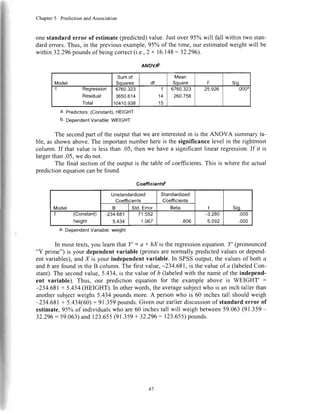
57. Chapter5 PredictionandAssociation
A multiple linear regressionwas calculatedto predict participants'weight
basedon their height and sex.A significantregressionequationwas found
(F(2,13): 981.202,p < .001),with an R' of .993.Participants'predicted
weightis equalto 47.138- 39.133(SEX)+ 2.10l(HEIGHT),whereSEX is
coded as I = Male, 2 : Female,and HEIGHT is measuredin inches.
Participantsincreased2.101 pounds for each inch of height, and males
weighed 39.133 pounds more than females.Both sex and height were
significantpredictors.
The conclusionstatesthe direction(increase),strength(.993),value(981.20),de-
greesof freedom(2,13),and significancelevel (< .001)of the regression.In addition,a
statementof the equationitself is included.Becausetherearemultiple independent vari-
ables,we havenotedwhetheror noteachis significant.
Phrasing ResultsThat Are Not Significant
If the ANOVA does not find a
significantrelationship,the Srg section
of the output will be greaterthan .05,
and the regressionequationis not sig-
nificant. A resultssectionfor the output
at right might include the following
statement:
A multiple linear regressionwas
calculated predicting partici-
pants'ACT scoresbasedon their
height and sex. The regression
equation was not significant
(F(2,13): 2.511,p > .05)withan
R" of .279. Neither height nor
weight is a significantpredictor
of lC7" scores.
llorlel Surrrwy
XodBl x R Souare
AdtuslBd
R Souare
Std Eror of
528. t68 3 07525
a Prsdlclors:(ConslanD.se4hel9ht
a Pr€dictors:(ConslanD,se( hsight
o.OoDendBnlVaiabloracl
Coetllclst 3r
Yodel
Unstandardizsd
Cosilcisnls
Standardized
Coeilcionts
stdSld E.rol Beia
I (Constan0
h€l9hl
s€x
oJttl
- 576
-t o??
19.88{
.266
2011
-.668
- 296
3.102
2.168
- s62
007
019
35{
Notethatforresultsthatare
"o,
,ir";;;;ilJlovA resultsandR2resultsare
given,buttheregressionequationisnot.
Practice Exercise
UsePracticeDataSet2 in AppendixB. Determinethepredictionequationfor pre-
dictingsalarybasedoneducation,yearsof service,andsex.Whichvariablesaresignificant
predictors?If you believethatmenwerepaidmorethanwomenwere,whatwouldyou
concludeafterconductingthisanalysis?
ANI]VIP
gumof
dt qin
I Reoressron
Rssidual
Total
1t.191
122.9a1
't70.t38
l3
't5
23.717
9.a57
2.5rI i tn.
52

58. Chapter6
ParametricInferentialStatistics
Parametricstatisticalproceduresallow you to draw inferencesaboutpopulations
basedon samplesof thosepopulations.To make theseinferences,you must be able to
makecertainassumptionsabouttheshapeof thedistributionsof thepopulationsamples.
Section6.1 Reviewof BasicHypothesisTesting
TheNull Hypothesis
In hypothesistesting,we createtwo hypothesesthat are mutually exclusive(i.e.,
bothcannotbe trueat thesametime)andall inclusive(i.e.,oneof themmustbe true).We
referto thosetwo hypothesesasthe null hypothesisandthe alternative hypothesis.The
null hypothesisgenerallystatesthatany differencewe observeis causedby randomerror.
The alternative hypothesisgenerallystatesthat any differencewe observeis causedby a
systematicdifferencebetweengroups.
TypeI andTypeII Eruors
All hypothesistestingattemptsto
draw conclusions about the real world
basedon the resultsof a test(a statistical
test,in this case).Thereare four possible
combinationsof results(seethe figure at <.r)
right). =
Two of thepossibleresultsarecor- A
rect test results.The other two resultsare
Uenors. A Type I error occurs when we ;
reject a null hypothesisthat is, in fact, fr
true, while a Type II error occurswhen l-
we fail to reject the null hypothesis that
is, in fact,false.
Significance tests determinethe
probabilityof makinga Type I error. In
otherwords,after performinga seriesof calculations,we obtaina probability that the null
hypothesisis true.If thereis a low probability,suchas5 or lessin 100(.05),by conven-
tion, we rejectthe null hypothesis.In otherwords,we typicallyusethe .05 level(or less)
asthemaximumType I error ratewe arewilling to accept.
Whenthereis a low probabilityof a Type I error, suchas.05,we canstatethatthe
significancetesthasled us to "rejectthe null hypothesis."This is synonymouswith say-
ing that a differenceis "statisticallysignificant."For example,on a readingtesr,suppose
you found thata randomsampleof girls from a schooldistrictscoredhigherthana random
zdi
6a
E-
-^6
6!u
trO
o>
'F:
n2
REALWORLD
NullHypothesisTrue NullHypothesisFalse
TypeI Error I NoError
NoError I Typell Error
53

59. Chapter6 ParametricInferentialStatistics
sampleof boys.This resultmay havebeenobtainedmerelybecausethe chanceenors as-
sociatedwith randomsamplingcreatedthe observeddifference(this is what the null hy-
pothesis asserts).If there is a sufficiently low probability that random errors were the
cause(asdeterminedby a significancetest),we canstatethatthe differencebetweenboys
andgirls is statisticallysignificant.
SignificanceLevelsvs.Critical Values
Moststatisticstextbookspresenthypothesistestingbyusingtheconceptof acriti-
cal value.With suchan approach,we obtaina valuefor a teststatisticand compareit to a
critical valuewe look up in a table.If theobtainedvalueis largerthanthe critical value,we
rejectthe null hypothesisandconcludethat we havefound a significantdifference(or re-
lationship).If the obtainedvalueis lessthanthecritical value,we fail to rejectthe null hy-
pothesisandconcludethatthereis not a significantdifference.
The critical-valueapproachis well suited to hand calculations.Tables that give
criticalvaluesfor alphalevelsof .001,.01,.05,etc.,canbe created.tt is not practicalto
createa tablefor everypossiblealphalevel.
On the other hand,SPSScan determinethe exactalpha level associatedwith any
valueof a teststatistic.Thus,lookingup a criticalvaluein a tableis not necessary.This,
however,doeschangethe basicprocedurefor determiningwhetheror not to rejectthe null
hypothesis.
The sectionof SPSSoutputlabeledSrg.(sometimesp or alpha) indicatesthe likeli-
hoodof makinga Type I error if we rejectthe null hypothesis.A valueof .05or lessin-
dicatesthatwe shouldrejectthe null hypothesis(assumingan alphalevel of .05).A value
greaterthan.05 indicatesthatwe shouldfail to rejectthe null hypothesis.
In other words, when using SPSS,we normally reject the null hypothesis if the
output value underSrg.is equalto or smallerthan .05, and we fail to reject the null hy-
pothesisif theoutputvalueis largerthan.05.
One-Tailed vs. Two-Tailed Tests
SPSSoutput generallyincludesa two-tailed alpha level (normally labeledSrg. in
the output).A two-tailed hypothesisattemptsto determinewhetherany difference(either
positiveor negative)exists.Thus,you havean opportunityto makea Type I error on ei-
therof thetwo tailsof thenormal distribution.
A one-tailedtestexaminesa differencein a specificdirection.Thus,we canmakea
Type I error on only oneside(tail) of the distribution.If we havea one-tailedhypothesis,
but our SPSSoutput gives a two-tailed significanceresult,we can take the significance
level in the outputanddivide it by two. Thus,if our differenceis in the right direction,and
if our output indicatesa significance level of .084 (two-tailed),but we have a one-tailed
hypothesis,we canreporta significancelevelof .042(one-tailed).
Phrasing Results
Resultsof hypothesistestingcanbe statedin differentways,dependingon the con-
ventionsspecifiedby your institution.The following examplesillustratesomeof thesedif-
ferences.
54

60. Chapter6 ParametricInferentialStatistics
Degreesof Freedom
Sometimesthe degreesof freedomare given in parenthesesimmediatelyafter the
symbolrepresentingthetest,asin thisexample:
(3):7.00,p<.01
Othertimes,the degreesof freedomaregiven within the statementof results,asin
thisexample:
t:7.00, df :3, p < .01
SignificanceLevel
When you obtain resultsthat are significant,they can be describedin different
ways.For example,if you obtaineda significancelevel of .006 on a t test,you
could describeit in any of the following threeways:
(3):7.00,p<.05
(3):7.00,p <.01
(3) : 7.00,p: .006
Noticethatbecausetheexactprobabilityis .006,both.05and.01arealsocorrect.
Therearealsovariouswaysof describingresultsthat arenot significant.For exam-
ple, if you obtaineda significancelevelof .505,any of the following threestate-
mentscouldbeused:
t(2): .805,ns
t(2):.805, p > .05
t(2)=.805,p:.505
Statementof Results
Sometimesthe resultswill be statedin termsof the null hypothesis,as in the fol-
lowing example:
Thenullhypothesiswasrejected1t: 7.00,df :3, p:.006).
Othertimes,the resultsarestatedin termsof their level of significance,asin the
followingexample:
A statisticallysignificantdifferencewasfound:r(3):7.00,p <.01.
StatisticalSymbols
Generally,statisticalsymbolsarepresentedin italics.Prior to the widespreaduseof
computersand desktoppublishing,statisticalsymbolswere underlined.Underlin-
ing is a signalto a printer that the underlinedtext shouldbe set in italics. Institu-
tions vary on their requirementsfor studentwork, so you are advisedto consult
your instructoraboutthis.
Section 6.2 Single-Sample I Test
Description
The single-sampleI testcomparesthe mean of a singlesampleto a known popula-
tion mean.It is usefulfor determiningif the currentsetof datahaschangedfrom a long-
I
55

61. Chapter6 ParametricInferentialStatistics
term value (e.g.,comparingthe curent year's temperaturesto a historical averageto de-
termineif globalwanning is occuning).
Assumptions
The distributionsfrom which the scoresare takenshouldbe normally distributed.
However,the t testis robust andcanhandleviolationsof the assumptionof a normal dis-
tribution. Thedependentvariablemustbemeasuredon aninterval or ratio scale.
.SP,SSData Format
The SPSSdatafile for the single-sample/ testrequiresa singlevariablein SPSS.
That variablerepresentsthe setof scoresin the samplethatwe will compareto the popula-
tion mean.
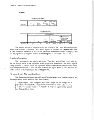
Running the Command
The single-sample/ testis locatedin the CompareMeanssubmenu,under theAna-
lyzemenu.The dialog box for the single-sample/ testrequiresthat we transferthevariable
representingthe currentsetofscores ry
to the Test Variable(s) section. We i ArdvzeGraphswllties
must also enterthe populationaver-
agein the TestValueblank.The ex-
ample presentedhere is testing the
variableLENGTH againsta popula-
tion meanof 35 (thisexampleusesa
hypotheticaldataset).
Reports )
I SescripliveStati*icr ]
GenerallinearModel )
' CorrElata )
' Regrossion )
Clasdfy )
Indegrdant-SrmplCsT
Paired-SamplesTTert.,,
0ne-WeyANOVA,..
ReadingtheOutput
The output for the single-samplet test consistsof two sections.The first section
lists the samplevariableand somebasicdescriptive statistics(N, mean, standard devia-
tion, andstandarderror).
Wiidnrunrb
Mcrns.,,
56

62. Chapter6 ParametricInferentialStatistics
T-Test
One-SampleTes{
TeslValue= 35
? df
sis.
(2-tailed)
Mean
DitTerence
95%gsnli6sngg
Interualofthe
Difierence
Lowef Upner
LENGTH 2.377 s .041 .9000 4.356E-02 7564
The secondsectionof output containsthe resultsof the t test. The examplepre-
sentedhereindicatesa / valueof 2.377,with 9 degreesof freedomanda significancelevel
of .041.The meandifferenceof .9000is thedifferencebetweenthe sampleaverage(35.90)
andthepopulationaveragewe enteredin thedialog box to conductthetest(35.00).
Drawing Conclusions
The I test assumesan equality of means.Therefore,a significant result indicates
that the samplemean is not equivalentto the populationmean (hencethe term "signifi-
cantlydifferent").A resultthatis not significantmeansthatthereis not a significantdiffer-
encebetweenthe means.It doesnot meanthat they areequal.Referto your statisticstext
for the sectionon failureto rejectthe null hypothesis.
PhrasingResultsThatAreSignificant
The aboveexamplefounda significantdifferencebetweenthepopulationmeanand
the samplemean.Thus,we couldstatethe following:
A single-samplet test comparedthe mean length of the sample to a
populationvalueof 35.00.A significantdifferencewas found (t(9) = 2.377,
p <.05).The samplemeanof 35.90(sd: 1.197)was significantlygreater
thanthepopulationmean.
One-SampleS'tatistics
N Mean
std.
Deviation
Std.Enor
Mean
LENGTH 10 35.9000 1.1972 .3786
57

63. Chapter6 ParametricInferentialStatistics
Phrasing ResultsThatAre Not Significant
If the significance level
hadbeengreaterthan .05,the dif-
ferencewould not be significant.
For example,if we receivedthe
output presentedhere, we could
statethe following:
A single-sample / test
comparedthe meantemp-
eratureover the past year
to the long-term average.
L'|D.S.Ittte Tesi
TsstValue= 57.1
t dt Sro (2-lail€d)
llean
DilTer€nce
95%Contldsnc6
Inlsryalofthe
Oit8rsnce
Lowsr UDOEI
lemp€latute I 688 1 ?6667 -5.7362 8.2696
The difference was not significant (r(8) = .417, p > .05). The mean
temperatureover the pastyearwas 68.67(sd = 9.1l) comparedto the long-
termaverageof 67.4.
Practice Exercise
The averagesalaryin the U.S. is $25,000.Determineif the averagesalaryof the
participantsin PracticeData Set 2 (AppendixB) is significantlygreaterthan this value.
Notethatthisis a one-tailedhypothesis.
Section6.3 Independent-samplesI Test
Description
The independent-samplesI testcomparesthe meansof two samples.The two sam-
plesarenormally from randomlyassignedgroups.
Assumptions
The two groupsbeingcomparedshouldbe independentof eachother.Observations
are independentwhen information about one is unrelatedto the other. Normally, this
meansthat onegroupof participantsprovidesdatafor onesampleanda differentgroupof
participantsprovides data for the other sample (and individuals in one group are not
matchedwith individualsin the othergroup).Oneway to accomplishthis is throughran-
dom assignmentto form two groups.
The scoresshouldbe normally distributed,but the I test is robust and can handle
violationsof theassumptionof a normal distribution.
The dependentvariable must be measuredon an interval or ratio scale.The in-
dependentvariable shouldhaveonly two discretelevels.
SP,S,SData Format
The SPSSdatafile for the independentI testrequirestwo variables.One variable,
the grouping variable, representsthe valueof the independentvariable. The grouping
variable shouldhavetwo distinct values(e.g.,0 for a control group and I for an experi-
L{n-S.I|pla Sl.llsllcs
N tean Sld Deviation
Std.Eror
tempetalure I OU.OODT 9.11013 3.03681
58

64. Chapter6 ParametricInferentialStatistics
mentalgroup).The secondvariablerepresentsthe dependentvariable, suchasscoreson a
test.
Conducting an Independent-Samples t Test
For our example,we will use
theSAMPLE.savdatafile.
Click Analyze, then Compare
Means, then Independent-SamplesT
?"est.This will bring up the main dia-
log box. Transfer the dependent
variable(s) into the Test Variable(s)
blank. For our example,we will use
[n;y* 6adrs Utltties window Heh
thevariableGRADL,.
TransfertheindependentvariableintotheGroupingVariablesection.Forourex-
ample,wewill usethevariableMORNING.
Next, click Define Groups and enter the
valuesof the two levels of the independent
variable. Independentt tests are capable of
comparingonly two levelsat a time. Click Con-
tinue,thenclick OK to run the analysis.
Outputfrom the Independent-Samples t Test
The outputwill havea sectionlabeled"Group Statistics."This sectionprovidesthe
basicdescriptivestatisticsfor thedependentvariable(s)for eachvalueof theindepend-
ent variable.It shouldlook like theoutputbelow.
GroupStatistics
mornrnq N Mean Std.Deviation
Std.Error
Mean
grade No
Yes
2
2
82.5000
78.0000
3.53553
7.07107
2.50000
5.00000
I
Can*bto
Regf6s$isl
ctaseff
)
l
t
'1
Std{ic* l ls elrl
it
dry
lim
mk
lr*iT
59

65. Chapter6 ParametricInferentialStatistics
Next, therewill be a sectionwith the resultsof the I test.It shouldlook like the
outputbelow.
lnd6pondent Samplo! Telt
Leveng's Tost for
Fdlralitv df Variencac ltest for Eoualitv of Msans
Sio. t df Sio.(2{ailed}
Mean
Diff6rence
Sld.Error
Ditforenc6
95% Confidenco
lntsrual of the
Diffor€nc6
Lower Uooer
graoe tqual vanances
assum6d
Equal variances
not assumed
.805
.805
2
1.471
505
530
4.50000
4.50000
5.59017
5.59017
-19.55256
-30.09261
28.55256
39.09261
The columnslabeledt, df, and Sig.(2-tailed)providethe standard"answer" for the
I test.They providethevalueof t, thedegreesof freedom(numberof participants,minus2,
in thiscase),andthe significancelevel(oftencalledp). Normally,we usethe "Equalvari-
ancesassumed"row.
Drawing Conclusions
Recall from the previous sectionthat the , test assumesan equality of means.
Therefore,a significantresult indicatesthat the meansare not equivalent.When drawing
conclusionsabouta I test,you muststatethedirectionof the difference(i.e.,which mean
was largerthan the other).You shouldalso include information about the value of t, the
degreesof freedom,thesignificancelevel,andthemeansandstandard deviationsfor the
two groups.
Phrasing ResultsThat Are Significant
For a significant/ test(for example,the outputbelow), you might statethe follow-
ing:
'.do,.ilhrh!
6adO slil|llk!
0r0uD N x€an Sld. Odiation
Sld Eror
xaan
sc0r9 conlfol
€rDoflmontal 3
al 0000 a.7a25a
2osr67
2 121J2
| 20185
hlapdrlra S,uplcr lcsl
Lmno's T€slfor
llasl for Fouellto ot lnans
Sid dT Sio a2-laile(n
xsan StdError
95(f,Contld9n.e
Inl€ryalofthe
sc0re EqualvarlencSs
assum€d
Equalvaiancos
nol assumgd
5058 071
31tl
5
a 53l
UJb
029
7 66667 2 70391
2138't2
71605
I 20060
I r.61728
rr.r3273
An independent-samplesI test comparing the mean scores of the
experimentaland control groupsfound a significant difference betweenthe
means of the two groups ((5) = 2.835,p < .05). The mean of the
experimentalgroupwas significantlylower (m = 33.333,sd:2.08) thanthe
meanof thecontrolgroup(m: 41.000,sd : 4.24).
60

66. Chapter6 ParametricInferentialStatistics
Phrasing ResultsThat Are Not Signifcant
In our exampleat the startof the section,we comparedthe scoresof the morning
peopleto the scoresof the nonmorningpeople.We did not find a significantdifference,so
we could statethe following:
An independent-samplest testwas calculatedcomparingthe meanscoreof
participantswho identifiedthemselvesasmorningpeopleto the meanscore
of participantswho did not identi$ themselvesas morning people. No
significant differencewas found (t(2) : .805,p > .05). The mean of the
morningpeople(m : 78.00,sd = 7.07)was not significantlydifferentfrom
themeanof nonmomingpeople(m = 82.50,sd= 3.54).
Practice Exercise
UsePracticeDataSetI (AppendixB) to solvethisproblem.We believethatyoung
individualshavelower mathematicsskills thanolder individuals.We would testthis hy-
pothesisby comparingparticipants25 or younger(the"young" group)with participants26
or older (the "old" group). Hint: You may needto createa new variable that represents
which agegroupthey arein. SeeChapter2 for help.
Section6.4 Paired-Samples/ Test
Description
The paired-samplesI test (also called a dependent/ test) comparesthe means of
two scoresfrom relatedsamples.For example,comparinga pretestanda posttestscorefor
a groupof participantswould requirea paired-samplesI test.
Assumptions
The paired-samplesI test assumesthat both variablesare at the interval or ratio
levelsand are normally distributed.The two variablesshould also be measuredwith the
samescale.If the scalesaredifferent.the scoresshouldbe convertedto z-scoresbeforethe
, testis conducted.
.SPSSData Format
Two variablesin the SPSSdatafile arerequired.Thesevariablesshouldrepresent
two measurementsfrom eachparticipant.
Running the Command
We will createa new datafile containingfive variables:PRETEST,MIDTERM,
FINAL, INSTRUCT, and REQUIRED. INSTRUCT representsthreedifferent instructors
for a course.REQUIRED representswhetherthe coursewas requiredor was an elective
(0 - elective,I : required).The otherthreevariablesrepresentexamscores(100 beingthe
highestscorepossible).
6l

67. Chapter6 ParametricInferentialStatistics
PRETEST
56
79
68
59
64
t.+
t)
47
78
6l
68
64
53
7l
6l
57
49
7l
6l
58
58
MIDTERM
64
9l
77
69
77
88
85
64
98
77
86
77
67
85
79
77
65
93
83
75
74
Enterthe dataand saveit as
GRADES.sav.You can checkyour
dataentryby computinga mean for
each instructor using the Means
command(seeChapter3 for more
information). Use INSTRUCT as
theindependentvariable andenter
PRETEST, MIDTERM, ANd
FINAL as your dependent vari-
ables.
Once you have enteredthe
data,conducta paired-samplesI test
comparing pretest scoresand final
scores.
Click Analyze, then Com-
pare Means,then Paired-SamplesT
?nesr.This will bring up the main
dialogbox.
i;vr*; 6r5db trl*lct
Bsi*i l
' l)06ctftlv.s44q t
@Cdnrdur*Modd t
FINAL
69
89
8l
7l
IJ
86
86
69
100
85
93
87
76
95
97
89
83
100
94
92
92
INSTRUCT
I
I
I
I
I
2
2
2
2
2
2
2
J
J
J
J
J
t
J
J
REQUIRED
0
0
0
0
0
0
0
0
0
tilkrdo| tbb
i c*@
i lryt'sn
i'w
Report
INSTRUCT PRETEST MIDTERM FINAL
1.00 Mean
N
std.
Deviation
67.5714
7
8.3837
(6.t'l4J
7
9.9451
79.5714
7
7.9552
2.00 Mean
N
std.
Deviation
63.1429
7
10.6055
79.1429
7
11.7108
86.4286
7
10.9218
3.00 Mean
N
std.
Deviation
59.2857
7
6.5502
78.0000
7
8.62',t7
92.4286
7
5.5032
Total Mean
N
std.
Deviation
63.3333
21
8.9294
78.6190
21
9.6617
86.1429
21
9.6348
q8-sdndo TTart...
62

68. Chapter6 ParametricInferentialStatistics
You must select pairs of
variablesto compare.As you se-
lect them, they are placed in the
Current Selectionsarea.
Click once on PRETEST.
then once on FINAL. Both vari-
ableswill be movedinto the Cnr-
rent Selectionsarea.Click on the
right anow to transferthe pair to
thePaired Variablessection.Click
OK to conductthetest.
Reading the Output
The output for
the paired-samplest test
consistsof three com-
ponents. The first part
givesyou basicdescrip-
tive statistics for the
PairedSamplesGorrelations
N Correlation Sio.
PaIT1 PRETEST
& FINAL 21 .535 .013
m
|y:tl
ry{l
.ry1
"l*;"J
: CundSdacti:n:
I VcirHal:
Vri{!ilcz
y.pllarq
*,n*f.n nCf;tndcim
ril',n*
atrirdftEl
d1;llqi.d
PairedSamplesStatistics
Mean N
std.
Deviation
Std.Error
Mean
Pair PRETEST
1 rtNet
63.3333
86.1429
21
21
8.9294
9.6348
1.9485
2.1025
xl
.!K I
"ttr.I-.tL*rd
i
fc
pairof variables.ThePRETESTaveragewas63.3,with a standarddeviationof 8.93.The
FINAL averagewas86.14,with a standarddeviationof 9.63.
I
The secondpartofthe
output is a Pearsoncorrela-
tion coefficientfor thepair of
variables.
Within the third partof the output(on the nextpage),the sectioncalledpaired Dif-
ferencescontainsinformationaboutthe differencesbetweenthe two variables.you miy
havelearnedin your statisticsclassthat the paired-samples/ test is essentiallya single-
samplet testcalculatedon thedifferencesbetweenthescores.The final threecolumnscon-
tain the value of /, the degreesof freedom,and the probability level. In the examplepre-
sentedhere,we obtaineda I of -11.646,with 20 degreesof freedomand a significance
levelof lessthan.00l. Notethatthis is a two-tailedsignificancelevel.Seethestartof this
chapterfor moredetailson computinga one-tailedtest.
PaildVaiibblt
63

69. Chapter6 ParametricInferentialStatistics
Paired Samples Test
Paired Differences
I df
sig
l)JailatlMean
srd,
Dcvirl
Std.Errot
Maan
95%Confidence
Inlervalof the
l)iffcrcncc
Lower UDoer
Pair1 PRETEST
. FINAL -22.8095 8.9756 1.9586 -26.8952 -18.7239 '|1.646 20 .000
Drawing Conclusions
Paired-samplesI testsdeterminewhetheror not two scoresare significantlydiffer-
ent from eachother. Significantvaluesindicatethat the two scoresare different. Values
thatarenot significantindicatethatthe scoresarenot significantlydifferent.
PhrasingResultsThatAreSignificant
When statingthe resultsof a paired-samplesI test,you shouldgive the valueof t,
the degreesof freedom,and the significancelevel.You shouldalso give the mean and
standard deviation for each variable.as well as a statementof resultsthat indicates
whetheryou conducteda one-or two-tailedtest.Our exampleabovewassignificant,sowe
couldstatethefollowing:
A paired-samplesI testwas calculatedto comparethe meanpretestscoreto
the meanfinal examscore.The meanon the pretestwas 63.33(sd : 8.93),
and the meanon the posttestwas 86.14(sd:9.63). A significantincrease
from pretestto final wasfound(t(20): -ll .646,p< .001).
Phrasing Results That Are Not Significant
If the significancelevelhadbeengreaterthan.05(or greaterthan.10 if you were
conductinga one-tailedtest),the resultwould not havebeensignificant.For example,the
hypotheticaloutputbelow representsa nonsignificantdifference.For this output,we could
state:
P.l crlSdr{ror St.rtlstkr
x6an N Sld Ddallon
Sld.Etrof
Patr midlsrm
1 nnal
rBt1a3
79.5711
7
I
I 9.509
795523
3 75889
3.00680
P.rl c(l Sxtlro3 Cq I olrlqt6
N Cotrelali 5to
ts4trI mtdt€rm&flnal I 96S 000
P.*od Silrlta! Tcrl
ParredOrflerences
tl Sio (2-lailad)xsan Std Oryiation
Std.Eror
X€an
95%ConidBncs
lnlsNrlotth€
DilYerenca
Lmt u008r
. 8571a 296808 I 12183 1 88788 - 76a b a7a
64

70. Chapter6 ParametricInferentialStatistics
A paired-samplest testwascalculatedto comparethemeanmidtermscoreto
themeanfinalexamscore.Themeanonthemidtermwas78.71(sd: 9.95),
andthemeanon thefinalwas79.57(sd:7.96). No significantdifference
frommidtermto finalwasfound((6) = -.764,p>.05).
Practice Exercise
UsethesameGRADES.savdatafile,andcomputea paired-samples/ testto deter-
mineif scoresincreasedfrommidtermto final.
Section6.5 One-Wav ANOVA
Description
Analysisof variance(ANOVA) is a procedurethatdeterminesthe proportionof
variabilityattributedto eachof severalcomponents.It is oneof themostusefulandadapt-
ablestatisticaltechniquesavailable.
Theone-wayANOVA comparesthemeansof two or moregroupsof participants
thatvary on a singleindependentvariable(thus,the one-waydesignation).Whenwe
havethreegroups,we couldusea I testto determinedifferencesbetweengroups,butwe
wouldhaveto conductthreet tests(GroupI comparedto Group2, GroupI comparedto
Group3, andGroup2 comparedto Group3).WhenweconductmultipleI tests,we inflate
the Type I error rateandincreaseour chanceof drawingan inappropriateconclusion.
ANOVA compensatesfor thesemultiplecomparisonsandgivesus a singleanswerthat
tellsusif anyof thegroupsisdifferentfromanyof theothergroups.
Assumptions
The one-wayANOVA requiresa singledependentvariable anda singleinde-
pendentvariable.Whichgroupparticipantsbelongto is determinedby thevalueof the
independentvariable.Groupsshouldbe independentof eachother.If our participants
belongto more than one group each,we will have to conducta repeated-measures
ANOVA. If we havemorethanoneindependentvariable,we wouldconducta factorial
ANOVA.
ANOVA alsoassumesthatthedependentvariableis attheintervalor ratio lev-
elsandisnormallydistributed.
SP,S,SData Format
Two variablesarerequiredin the SPSSdatafile. Onevariableservesasthede-
pendentvariableandtheotherastheindependentvariable.Eachparticipantshouldpro-
videonlyonescorefor thedependentvariable.
RunningtheCommand
Forthisexample,wewill usetheGRADES.savdatafile wecreatedin theprevious
section.
65

71. Chapter6 ParametricInferentialStatistics
To conducta one-wayANOVA, click Ana-
lyze, then CompareMeans, then One-I7ayANOVA.
This will bring up the main dialog box for theOne-
lltayANOVA command.
xrded
f *wm
dtin"t
S instt.,ct
/ rcqulad
miqq|4^__
l':lirl:.,.
:J
f,'',I
R*gI
c*"d I
HdpI
i An$tea &ryhr l.{lith;
R;pa*tr )
DrrsFfivsft#l|' I
Csnalda
R!E'l'd6al
cl#y
lhcd friodd ] orn-5dtFh f f64...
I l|1|J46tddg.5arylarT16t,.,
) P*G+tunpbs I IcJt..,
rffillEil
wr$|f $alp
!qt5,l fqiryt,,,lodiors"'I
pela$t
/n*Jterm
d
'cqfuda
mrffi,.*-
-rl
ToKl
Ro"t I
c*ll
H&l
"?s'qt,.,l
Pqyg*-I odi"*.'.I
Click on the Options box to
get the Options dialog box. Click
Descriptive. This will give you
meansfor thedependentvariableat
eachlevel of the independentvari-
able. Checkingthis box preventsus
from having to run a separatemeans
command.Click Continueto return
to the main dialog box. Next, click
Post Hoc to bring up the Post Hoc
Multiple Comparisonsdialog box.
Click Tukev.thenContinue.
, Eqiolvdirnccs NotfudfiEd
.
r TY's,T2
l,?."*:,_: _l6{''6:+l.'od
t or*ol:: j
Sigflber! h,v!t tffi-
rc"'*i.'I r"ry{-l" H* |
Post-hoctestsare necessaryin the event of a significant ANOVA. The ANOVA
only indicatesif any groupis differentfrom any othergroup.If it is significant,we needto
determinewhich groupsaredifferent from which othergroups.We could do I teststo de-
terminethat,but we would havethe sameproblemasbeforewith inflating the Type I er-
ror rate.
Thereare a variety of post-hoccomparisonsthat correctfor the multiple compari-
sons.The most widely usedis Tukey's HSD. SPSSwill calculatea varietyof post-hoc
testsfor you. Consultanadvancedstatisticstext for a discussionof the differencesbetween
thesevarioustests.Now click OK to run the analvsis.
You shouldplacethe independ-
ent variable in the Factor box. For our
example, INSTRUCT representsthree
different instructors.and it will be used
asour independentvariable.
Our dependentvariable will be
FINAL. This test will allow us to de-
termine if the instructorhas any effect
on final sradesin thecourse.
f- Fncdrdr*dcndlscls
l* Honroga&olvairre,* j *_It J
66

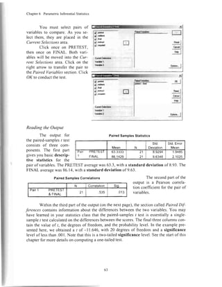
72. Chapter6 ParametricInferentialStatistics
ReadingtheOutput
Descriptivestatisticswill begivenfor eachinstructor(i.e.,levelof theindepend-
entvariable)andthetotal.Forexample,in hisftrerclass,InstructorI hadanaveragefinal
examscoreof 79.57.
Descriptives
final
N Mean Std.Deviation Std.Enor
95%ConfidenceIntervalfor
Mean
Minimum MaximumLowerBound UooerBound
UU
2.00
3.00
Total
7
7
2'l
79.5714
86.4286
92.4286
86.1429
7.95523
10.92180
5.50325
9.63476
3.00680
4.12805
2.08003
2.10248
72.2',t41
76.3276
87.3389
81.7572
86 9288
96.5296
97.5182
90.5285
tiv.uu
69.00
83.00
69.00
6Y.UU
100.00
100.00
100.00
The next sectionof
the output is the ANOVA
sourcetable.This is where
the various componentsof
the variance have been
listed,alongwith their rela-
tive sizes.For a one-wayANOVA, thereare two componentsto the variance:Between
Groups(which representsthe differencesdue to our independentvariable) and Within
Groups(whichrepresentsdifferenceswithin eachlevelof our independentvariable).For
our example,the BetweenGroupsvariancerepresentsdifferencesdue to different instruc-
tors.The Within Groupsvariancerepresentsindividualdifferencesin students.
The primaryansweris F. F is a ratio of explainedvariance to unexplainedvari-
ance.Consulta statisticstext for moreinformationon how it is determined.The F hastwo
differentdegreesof freedom,onefor BetweenGroups(in this case,2is the numberof lev-
elsof our independentvariable [3 - l]), andanotherfor Within Groups(18 is thenumber
of participantsminusthenumberof levelsof our independentvariable [2] - 3]).
The next part of the output consistsof the resultsof our Tukey's ^EISDpost-hoc
comparison.
This tablepresentsus with everypossible
ent variable. The first row representsInstructor
structor I compared to
Instructor 3. Next is In- Dooendenrvariabre:F,NAL
structor 2 compared to
Instructor l. (Note that
this is redundantwith the
first row.) Next is Instruc-
tor 2 comparedto Instruc-
tor 3, andsoon.
The column la-
beled Sig. representsthe
Type I error (p) rate for
the simple(2-level)com-
parisonin that row. In our
combinationof levelsof our independ-
I comparedto Instructor2. Next is In-
Multlple Comparlsons
579.429
1277.143
1856.571
HSD
(t) (J)
INSTRUCT INSTRUCT
Mean
Difference
Il-.tl Sld. Enor Sia
95% Confidence
Lower
Bound
Upper
R6r rn.l
1.00 2.OU
3.00
€.8571
-12.8571'
4.502
4.502
JU4
.027
-16.J462
-24.3482
4.6339
-1.3661
2.00 1.00
3.00
6.8571
-6.0000
4.502
4.502
.304
.396
-4.6339
-17.4911
18.3482
5,4911
3.00 1.00
2.00
12.8571'
6.0000
4.502
4.502
.027
.396
1.3661
-5.4911
24.3482
17.4911
'. The meandiffer€nceis significantat the .05 level.
67

73. Chapter6 ParametricInferentialStatistics
exampleabove,InstructorI is significantlydifferentfromInstructor3, but InstructorI is
not significantlydifferentfromInstructor2, andInstructor2 is not significantlydifferent
fromInstructor3.
Drawing Conclusions
Drawing conclusionsfor ANOVA requiresthat we indicatethe value of F, the de-
greesof freedom,andthe significancelevel.A significantANOVA shouldbe followed by
theresultsof a post-hocanalysisanda verbalstatementof the results.
Phrasing ResultsThat Are Significant
In our exampleabove,we couldstatethefollowing:
We computed a one-way ANOVA comparing the final exam scoresof
participantswho took a coursefrom one of three different instructors.A
significant differencewas found among the instructors(F(2,18) : 4.08,
p < .05).Tukey's f/SD was usedto determinethe natureof the differences
between the instructors.This analysis revealed that studentswho had
InstructorI scoredlower (m:79.57, sd:7.96) than studentswho had
Instructor3 (m = 92.43,sd: 5.50).Studentswho hadInstructor2 (m:86.43,
sd : 10.92)were not significantlydifferent from either of the other two
groups.
Phrasing ResultsThat Are Not Significant
If we hadconductedthe
analysis using PRETEST as
our dependent variable in-
stead of FINAL, we would
have received the following
output:
The ANOVA was not signifi-
cant. so thereis no needto re-
fer to the Multiple Compari-
sons table. Given this result,
we may statethe following:
The pretest means of students who took a course from three different
instructors were compared using a one-way ANOVA. No significant
differencewas found(F'(2,18)= 1.60,p >.05).The studentsfrom the three
differentclassesdid not differ significantlyat the startof the term. Students
who had InstructorI had a meanscoreof 67.57(sd : 8.38).Studentswho
had Instructor2 had a meanscoreof 63.14(sd : 10.61).Studentswho had
lnstructor3 hada meanscoreof 59.29(sd= 6.55).
Ocrcrlriir
N Sld Ddaton Sld Eiror
95$ Conlldanc0 Inloml tol
LMf Bound Uooer gound
200
300
Tolel
1
21
63.1r29
592857
633333
10.605r8
6.55017
I 92935
4.00819
2.at5t1
I ga€sa
5333ra
532278
592587
7?95r3
55 3a36
67 3979
1700
r9.00
at 00
7800
7100
7900
All:'Vl
sumof
210.667
135a.000
t 594667
t8
20
120333
15222
1 600 229
wrlhinOroups
Tol.l
68

74. Chapter6 ParametricInferentialStatistics
Practice Exercise
UsingPracticeDataSetI in AppendixB, determineif theaveragemathscoresof
single,married,anddivorcedparticipantsaresignificantlydifferent.Writea statementof
results.
Section6.6 Factorial ANOVA
Description
ThefactorialANOVA is onein whichthereis morethanoneindependentvari-
able.A 2 x 2 ANOVA, for example,hastwo independentvariables,eachwith two lev-
els.A 3 x 2 x 2 ANOVA hasthreeindependentvariables.Onehasthreelevels,andthe
othertwo havetwo levels.FactorialANOVA is verypowerfulbecauseit allowsusto as-
sesstheeffectsof eachindependentvariable,plustheeffectsof theinteraction.
Assumptions
FactorialANOVA requiresall of theassumptionsof one-wayANOVA (i.e.,the
dependentvariablemustbeat theinterval or ratio levelsandnormallydistributed).In
addition,theindependentvariablesshouldbeindependentof eachother.
.SPSSData Format
SPSSrequiresonevariablefor thedependentvariable,andonevariablefor each
independentvariable.If wehaveanyindependentvariablethatis representedasmulti-
ple variables(e.g.,PRETESTand POSTTEST),we must use the repeated-measures
ANOVA.
RunningtheCommand
This exampleusesthe GRADES.sav
file fromearlierin thischapter.ClickAna-
thenGeneralLinearModel.thenUnivari-
This will bring up the main dialog
box for Univariate ANOVA. Select the
dependent variable and place it in the
DependentVariableblank (useFINAL for
this example). Select one of your inde-
pendent variables (INSTRUCT, in this
case)and place it in the Fixed Factor(s)
box. Placethe secondindependentvari-
able (REQUIRED) in the Fixed Factor(s)
data
lyze,
ate.
I RnalyzeGraphs
Repsrts
USiUasllilindow Halp
DescrbtiwStatFHcs
!!{4*,l
?**" I
-..fP:.J
fi*"qrJ
!t,, I
9*ll
R{'dsr! F.dclt}

75. Chapter6 ParametricInferentialStatistics
box. Having defined the analysis, now click
Options.
When the Options dialog box comes up,
move INSTRUCT, REQUIRED, and INSTRUCT
x REQUIRED into the Display Meansfor blank.
This will provide you with means for each main
effectandinteraction term.Click Continue.
If you wereto selectPost-Hoc,SPSSwould
run post-hocanalysesfor the main effectsbut not
for the interaction term. Click OK to run the
analvsis.
1.INSTRUCT
Reading the Output
At the bottom of the
output, you will find the means
for each main effect and in-
teraction you selectedwith the
Optionscommand.
There were three
instructors, so there is a mean
FINAL for each instructor. We
also have means for the two
values of REQUIRED. FinallY,
we have six means representing
the interaction of the two
variables (this was a 3 x 2
design).
Participants who had
Instructor I (for whom the class
was not required)had a mean final exam scoreof 79.67.Studentswho had Instructor I
(for whom it wasrequired)hada mean final examscoreof 79.50,andsoon.
The examplewe just
ran is called a two-way
ANOVA. This is becausewe
had two independentvari-
ables. With a two-way
ANOVA, we get three an-
swers: a main effect for
INSTRUCT, a main effect
for REQUIRED, and an in-
teraction result for
INSTRUCT ' REQUIRED
(seetop ofnext page).
2. REQUIRED
ariable:FINAL
REOUIRED Mean Std.Error
95%ConfidenceInterval
Lower
Rorrnd
Upper
Bound
,UU
1.00
84.667
87.250
3.007
2.604
78.257
81.699
91.076
92.801
3.INSTRUCT'REQUIRED
Variable:FINAL
INSTRUCTREQUIRED Mean Std.Error
95%ConfidenceInterval
Lower
Bound
Upper
Bound
1.00 .00
1.00
79.667
79.500
5.208
4.511
68.565
69.886
90.768
89.114
2.00 .00
1.00
84.667
87.750
5.208
4.511
73.565
78.136
95.768
97.364
3.00 .00
1.00
89.667
94.500
5.208
4.511
78.565
84.886
100.768
104.114
ariable:FINAL
INSTRUCT Mean Std.Error
95oloConfidencelnterval
Lower
Bound
Upper
Bound
1.UU
2.00
3.00
79.583
86.208
92.083
3.445
3.445
3.445
72.240
78.865
84.740
86.926
93.551
99.426
70

76. Chapter6 ParametricInferentialStatistics
Tests of Between-SubjectsEffects
DependentVariable:FINAL
a. R Squared= .342(AdjustedR Squared= .123)
The source-table above gives us these three answers (in the INSTRUCT,
REQUIRED, and INSTRUCT * REQUIRED rows). In the example,noneof the main ef-
fectsor interactions wassignificant.tn the statementsof results,you must indicate^F,two
degreesof freedom(effect and residual/error),the significance'level, and a verbal state-
ment for eachof the answers(three,in this case).uite that most statisticsbooks give a
much simpler versionof an ANOVA sourcetable where the CorrectedModel, Intercept,
andCorrectedTotal rows arenot included.
Phrasing ResultsThat Are Significant
If we hadobtainedsignificantresultsin this example,we could statethe following
(Theseare fictitious results.For the resultsthat corresponato the exampleabove,please
seethesectionon phrasingresultsthatarenot significant):
A 3 (instructor)x 2 (requiredcourse)between-subjectsfactorial ANOVA
wascalculatedcomparingthe final examscoresfor participantswho hadone
of threeinstructorsandwho took the courseeitherasa requiredcourseor as
an elective.A significantmain effect for instructorwas found (F(2,15) :
l0.ll2,p < .05).studentswho hadInstructorI hadhigherfinal .*u- r.o16
(m = 79.57,sd:7.96) thanstudentswho hadInstructor3 (m:92.43, sd:
5.50). Studentswho had Instructor2 (m : g6.43,sd :'10.92) weie not
significantlydifferentfrom eitherof theothertwo groups.A significantmain
effectfor whetheror not thecoursewasrequiredwasfound(F(-1,15):3g.44,
p < .01)'Studentswho took thecoursebecauseit wasrequireddid better(z :
9l '69,sd: 7.68)thanstudentswho tookthecourseasanelective (m : 77.13,
sd:5.72). Theinteractionwasnotsignificant(F(2,15)= l.l5,p >.05). The
effectof the instructorwasnot influencedby whetheror not thestudentstook
thecoursebecauseit wasrequired.
Note that in the aboveexampre,we would have had to conductTukey,s HSD to
determinethe differencesfor INSTRUCT (using thePost-Hoccommand).This is not nec-
Intercept
INSTRUCT
REQUIRED
INSTRUCT' REQUIRED
Error
Total
CorrectedTotal
635.8214
1s1998.893
536.357
34.32'l
22.071
1220.750
157689.000
1856.571
5
1
2
1
2
15
21
20
151998.893
268.179
34.321
11.036
81.383
1867.691
3.295
.422
.136
.000
.065
.526
.874
7l

77. Chapter6 ParametricInferentialStatistics
Testsof Between-SubjectsEffects
t Variable:FINAL
Source
Typelll
Sumof
Souares df
Mean
Souare F siq.
uorrecleoMooel
Intercept
INSTRUCT
REQUIRED
INSTRUCT- REQUIRED
Error
Total
CorrectedTotal
635.8214
151998.893
536.357
34.321
22.071
1220.750
157689.000
't856.571
5
1
2
1
2
1E
21
20
127.164
151998.893
268.179
34.321
11.036
81.383
1.563
1867.691
3.295
.422
.136
.230
.000
.065
.526
.874
a. R Squared= .342(AdjustedR Squared= .123)
The source table above gives us these three answers (in the INSTRUCT,
REQUIRED,andINSTRUCT * REQUIREDrows).In the example,noneof the mainef-
fectsor interactions was significant.In the statementsof results,you must indicatef', two
degreesof freedom(effect and residual/error),the significance level, and a verbal state-
ment for eachof the answers(three,in this case).Note that most statisticsbooksgive a
much simplerversionof an ANOVA sourcetablewherethe CorrectedModel, Intercept,
andCorrectedTotal rows arenot included.
Phrasing ResultsThat Are Signifcant
If we hadobtainedsignificantresultsin thisexample,we couldstatethe following
(Theseare fictitiousresults.For the resultsthatcorrespondto the exampleabove,please
seethesectionon phrasingresultsthatarenot significant):
A 3 (instructor)x 2 (requiredcourse)between-subjectsfactorial ANOVA
wascalculatedcomparingthe final examscoresfor participantswho hadone
of threeinstructorsandwho took the courseeitherasa requiredcourseor as
an elective.A significantmain effect for instructorwas found (F(2,15 :
l0.l 12,p < .05).Studentswho hadInstructorI hadhigherfinal examscores
(m : 79.57,sd : 7.96)thanstudentswho had Instructor3 (m : 92.43,sd :
5.50). Studentswho had Instructor2 (m : 86.43,sd : 10.92) were not
significantlydifferentfrom eitherof theothertwo groups.A significantmain
effectfor whetheror not thecoursewasrequiredwasfound(F'(1,15):38.44,
p < .01).Studentswho took thecoursebecauseit wasrequireddid better(ln :
91.69,sd:7.68) thanstudentswho tookthecourseasanelective(m:77.13,
sd : 5.72).The interactionwasnot significant(,F(2,15): I .15,p > .05).The
effectof the instructorwasnot influencedby whetheror not the studentstook
thecoursebecauseit wasrequired.
Note that in the aboveexample,we would havehad to conductTukey's HSD to
determinethe differencesfor INSTRUCT (usingthePost-Hoccommand).This is not nec-
71

78. Chapter6 ParametriclnferentialStatistics
essaryfor REQUIREDbecauseit hasonlytwo levels(andonemustbedifferentfromthe
other).
Phrasing ResultsThatAre Not Significant
Ouractualresultswerenotsignificant,sowecanstatethefollowing:
A 3 (instructor)x 2 (requiredcourse)between-subjectsfactorialANOVA
wascalculatedcomparingthefinalexamscoresfor participantswhohadone
of threeinstructorsandwho tookthecourseasa requiredcourseor asan
elective.Themaineffectfor instructorwasnotsignificant(F(2,15): 3.30,p
> .05).Themaineffectfor whetheror notit wasa requiredcoursewasalso
notsignificant(F(1,15)= .42,p> .05).Finally,theinteractionwasalsonot
significant(F(2,15)= .136,p > .05). Thus,it appearsthat neitherthe
instructornorwhetheror notthecourseis requiredhasanysignificanteffect
onfinalexamscores.
Practice Exercise
UsingPracticeDataSet2 in AppendixB, determineif salariesareinfluencedby
sex,job classification,or aninteractionbetweensexandjob classification.Writea state-
mentof results.
Section6.7 Repeated-MeasuresANOVA
Description
Repeated-measuresANOVA extendsthe basicANOVA procedureto a within-
subjectsindependentvariable(whenparticipantsprovidedatafor morethanonelevelof
an independentvariable).It functionslike a paired-samples/ testwhenmorethantwo
levelsarebeingcompared.
Assumptions
Thedependentvariableshouldbenormallydistributedandmeasuredonaninter-
val or ratio scale.Multiplemeasurementsof thedependentvariableshouldbefromthe
same(orrelated)participants.
SP,S^SData Format
At leastthreevariablesarerequired.Eachvariablein theSPSSdatafile shouldrep-
resenta singledependentvariableata singlelevelof theindependentvariable'Thus,an
analysisof a designwith fourlevelsof anindependentvariablewouldrequirefourvari-
ablesin theSPSSdatafile.
If anyvariablerepresentsa between-subjectseffect,usetheMixed-DesignANOVA
commandinstead.
72

79. Chapter6 ParametricInferentialStatistics
RunningtheCommand
ThisexampleusestheGRADES.savsample
dataset.Recallthat GRADES.savincludesthree
sets of grades-PRETEST, MIDTERM, and
FINAL-that representthreedifferenttimesduring
thesemester.This allowsusto analyzetheeffects
of time on the test performanceof our sample
population(hencethe within-groupscomparison).
Click Analyze,thenGeneralLinear Model, then
W,;,
Ui**tSubioctFactorNanc ffi*
Nr,nrbarqllcv6ls: l3*
--J
ltl
'@ !8*vxido"'
t{!idf-!de r $.dryrigp,,,
RepeatedMeasures.
Note that this procedure requires an optional module. If you do not have this
command,you do not have theproper module installed. Thisprocedure is NOT included
in the student version o/SPSS.
Mea*lxaNsre: I
After selectingthe command,you will be
presented with the Repeated Measures Define
Factor(s)dialog box. This is where you identify the
within-subjectfactor(we will call it TIME). Enter3
for thenumberof levels(threeexams)andclickAdd.
Now click Define.If we had more than one
independentvariable that had repeatedmeasures,
we couldenterits nameandclick Add.
You will be presentedwith the Repeated
Measures dialog box. Transfer PRETEST,
MIDTERM, and FINAL to the lhthin-Subjects
Variables section. The variable names should be
orderedaccordingto whentheyoccurredin time(i.e.,
the valuesof the independent variable that they
represent).
Click Options,andSPSSwill computethe meansfor theTIME effect(seeone-way
ANOVA for moredetailsabouthow to do this).Click OK to run the command.
-xl
,,.,. I
B"*,I
cr,ca I
Hsl
f,txrd*r )
gp{|ssriori
tSoar
garlrr! Cffiporur&'..
h{lruc{ l'or I
-Ff?l
-9v1"I
-ssl
U"a* | cro,r"*.I nq... I pagoq..I S""a..I geb*.. I
/J

80. Chapter6 ParametricInferentialStatistics
ReadingtheOutput
This procedureusestheGLM command.
GLM standsfor "GeneralLinearModel."It is a
very powerfulcommand,and manysectionsof
outputarebeyondthescopeofthis text(seeout-
put outlineat right).But for the basicrepeated-
measuresANOVA, we areinterestedonly in the
Testsof l{ithin-SubjectsEffects.Note that the
SPSSoutputwill includemanyothersectionsof
output,whichyoucanignoreatthispoint.
Title
Notes
Wlthin-Subjects Factors
MultivariateTests
Mauchly'sTes{ol Sphericity
Testsol Wthin-SubjectsEflecls
Tesisol /lthin-SubjectsContrasts
Testsol Between-SubjectsEllec{s
fil sesso,.rtput
H &[ GeneralLinearModel
Tests of WrllrilFstil)iectsEffecls
Measure:MEASURE1
Source
TypelllSum
ofSouares df MeanSouare F Siq.
time SphericityAssumed
Greenhouse-Geisser
Huynh-Feldt
Lower-bound
5673.746
5673.746
5673.746
5673.746
2
1.211
1.247
1.000
2836.873
4685.594
4550.168
5673.746
121.895
121.895
121.895
121.895
000
000
000
000
Error(time)SphericityAssumed
Greenhouse-Geisser
Huynh-Feldt
Lower-bound
930.921
930.921
930.921
930.921
40
24.218
24.939
20.000
23.273
38.439
37.328
46.546
The TPeslsof l{ithin-SubjectsEffectsoutputshouldlook very similarto theoutput
from the otherANOVAcommands.In theaboveexample,theeffectof TIME hasanF
valueof 121.90with 2 and40 degreesof freedom(we usethe line for SphericityAs-
sumed).It is significantat lessthanthe .001level.Whendescribingtheseresults,we
shouldindicatethetypeof test,F value,degreesof freedom,andsignificancelevel.
Phrasing ResultsThatAre Significant
BecausetheANOVA resultsweresignificant,weneedto dosomesortof post-hoc
analysis.One of the main limitationsof SPSSis the difficulty in performingpost-hoc
analysesfor within-subjectsfactors.With SPSS,theeasiestsolutionto thisproblemis to
conductprotecteddependentt testswith repeated-measuresANOVA. Therearemore
powerful(andmoreappropriate)post-hocanalyses,but SPSSwill not computethemfor
us.Formoreinformation,consultyourinstructoror amoreadvancedstatisticstext.
To conductthe protectedt tests,we will comparePRETESTto MIDTERM,
MIDTERMto FINAL,andPRETESTto FINAL,usingpaired-samplesI tests.Becausewe
areconductingthreetestsand,therefore,inflatingourTypeI error rate,wewill usea sig-
nificancelevelof .017(.05/3)insteadof .05.
74

81. Chapter6 ParametricInferentialStatistics
Paired Samples Test
PairedDifferences
df
sig
{2-tailed)Mean
std.
Dcvietior
Std.Error
Mean
950/oConfidence
Intervalofthe
l)ifferance
Lower UoDer
Yatr 1 l,KE I E5 |
MIDTERM
Pai 2 PRETEST
. FINAL
Pair3 MIDTERM
. FINAL
-15.2857
-22.8095
-7.5238
3.9641
8.97s6
6.5850
.8650
1.9586
1.4370
-17.0902
-26.8952
-10.5213
-13.4813
-18.7239
4.5264
-'t7.670
-11.646
-5.236
20
20
20
.000
.000
.000
The threecomparisonseachhada significancelevel of lessthan.017, so we can
concludethat the scoresimprovedfrom pretestto midterm and again from midterm to fi-
nal. To generatethe descriptive statistics,we haveto run the Descriptivescommandfor
eachvariable.
Becausethe resultsof our exampleaboveweresignificant,we could statethe fol-
lowing:
A one-wayrepeated-measuresANOVA was calculatedcomparingthe exam
scoresof participantsat threedifferenttimes:pretest,midterm,and final. A
significanteffect was found (F(2,40) : 121.90,p < .001). Follow-up
protectedI testsrevealedthatscoresincreasedsignificantlyfrom pretest(rn:
63.33,sd: 8.93)to midterm(m:78.62, sd:9.66), andagainfrommidterm
to final(m= 86.14,sd:9.63).
Phrasing ResultsThat Are Not Significant
With resultsthatarenot significant,we couldstatethefollowing(theF valueshere
havebeenmadeup for purposesof illustration):
A one-wayrepeated-measuresANOVA wascalculatedcomparingthe exam
scoresof participantsat threedifferenttimes:pretest,midterm,and final. No
significant effect was found (F(2,40) = 1.90,p > .05). No significant
differenceexistsamongpretest(m: 63.33,sd = 8.93),midterm(m:78.62,
sd:9.66), andfinal(m:86.14, sd: 9.63)means.
Practice Exercise
Use PracticeData Set 3 in Appendix B. Determineif the anxiety level of partici-
pantschangedover time (regardlessof which treatmentthey received)using a one-way
repeated-measuresANOVA andprotecteddependentI tests.Write a statementof results.
Section 6.8 Mixed-Design ANOVA
Description
The mixed-designANOVA (sometimescalled a split-plot design)teststhe effects
of morethanoneindependentvariable.At leastoneof the independentvariablesmust
75

82. Chapter6 ParametricInferentialStatistics
be within-subjects(repeatedmeasures).At leastoneof theindependentvariablesmustbe
between-subjects.
Assumptions
The dependentvariable shouldbe normallydistributedandmeasuredon an inter-
val or ratio scale.
SPSSData Format
The dependentvariable shouldbe representedasonevariablefor eachlevelof the
within-subjectsindependentvariables.Anothervariableshouldbe presentin the datafile
for eachbetween-subjectsvariable.Thus, a 2 x 2 mixed-designANOVA would require
threevariables,two representingthe dependentvariable (oneat eachlevel),and onerep-
resentingthebetween-subjectsindependentvariable.
Running the Command
The GeneralLinear Model commandruns
the Mixed-Design ANOVA command. Click Ana-
lyze, then General Linear Model, then Repeated
Measures.Note that this procedure requires an
optional module. If you do not have this com-
mand, you do not have the proper module in-
stalled. This procedure is NOT included in the
student version o/,SPSS.
The RepeatedMeasurescommand
shouldbe usedif any of the independent
variables are repeatedmeasures(within-
subjects).
This example also uses the
GRADES.savdata file. Enter PRETEST,
MIDTERM, and FINAL in the lhthin-
Subjects Variables block. (See the
RepeatedMeasuresANOVA commandin
Section 6.7 for an explanation.)This
exampleis a 3 x 3 mixed-design.There
are two independent variables (TIME
and INSTRUCT), eachwith three levels.
We previouslyenteredthe informationfor
TIME in the RepeatedMeasuresDefine
Factorsdialogbox.
Cocpa''UF46 )
@
ilrGdtilod6b )
iifr.{*r }
&rfcrgon l
tAdhraf i
lAnqtr:l g{hs Udear
Rqprto
r oitc|hfiy. $rtBtlca
i T.d*t
gfitsrf*|drvdbbht
Add-gnr Uhdorn
IK
terI
s*i I
t*.,
34 1
mT-
Uoo*..I cotrl... I 8q... I Podg*.I Sm.. | 8e4.. I
We needto transferINSTRUCT into theBetween-SubjectsFactor(s)block.
Click Optionsandselectmeansfor all of the main effectsand the interaction (see
one-wayANOVA in Section6.5 for more detailsabouthow to do this). Click OK to run
thecommand.
76

83. f
Chapter6 ParametricInferentialStatistics
ReadingtheOutput
As with thestandardrepeatedmeasurescommand,theGLM procedureprovidesa
lot of outputwe will notuse.Fora mixed-designANOVA, we areinterestedin two sec-
tions.Thefirst is Testsof Within-SubjectsEffects.
Testsot Wrtlrilr-SuuectsEflects
Measure:
Source
TypelllSum
ofSquares df MeanSouare F sis
time sphericityAssumed
Greenhouse-Geissel
Huynh-Feldt
Lower-bound
5673.746
5673.746
5673.746
5673.746
-2
1.181
1.356
1.000
2836.873
4802.586
4't83.583
5673.746
817.954
817.954
817.954
817.954
000
000
000
000
time' instruct SphericilyAssumed
0reenhouse-Geisser
Huynh-Feldt
Lower-bound
806.063
806.063
806.063
806.063
4
2.363
2.f't2
2.000
201.516
341.149
297.179
403.032
58.103
58.103
58.103
58.103
.000
.000
.000
.000
Erro(time) SphericityAssumed
Greenhouse-Geisser
Huynh-Feldt
Lower-bound
124857
124.857
124.857
124.857
36
21.265
24.41'.|
18.000
3.468
5.871
5.115
6.S37
This sectiongivestwo of the threeanswerswe need(themain effect for TIME and
the interactionresultfor TIME x INSTRUCTOR).The secondsectionof outputis Testsof
Between-subjectsEffects(sampleoutput is below). Here, we get the answersthat do not
contain any within-subjects effects. For our example, we get the main effect for
INSTRUCT. Both of thesesectionsmust be combinedto oroducethe full answerfor our
analysis.
Testsot Betryeen-Sill)iectsEltecls
Measure:MEASURE1
ransformedVariable:
Source
TypelllSum
ofSquares df MeanSouare F Siq.
Intercepl
inslrucl
Enor
364192.063
18.698
4368.571
I
2
18
364192.063
9.349
242.6S8
1500.595
.039
.000
.962
If we obtain significanteffects,we must perform somesort of post-hocanalysis.
Again, this is oneof the limitationsof SPSS.No easyway to performthe appropriatepost-
hoc test for repeated-measures(within-subjects)factorsis available.Ask your instructor
for assistancewith this.
When describingthe results,you shouldincludeF, the degreesof freedom,andthe
significancelevel for eachmain effectandinteraction.In addition,somedescriptivesta-
tisticsmustbe included(eithergivemeansor includea figure).
Phrasing ResultsThat Are Significant
There are threeanswers(at least)for all mixed-designANOVAs. PleaseseeSec-
tion 6.6 on factorialANOVA for moredetailsabouthow to interpretandphrasetheresults.
77

84. Chapter6 ParametricInferentialStatistics
For the aboveexample,we could statethe following in the resultssection(notethatthis
assumesthatappropriatepost-hoctestshavebeenconducted):
A 3 x 3 mixed-designANOVA wascalculatedto examinethe effectsof the
instructor(Instructors1,2, and,3)and time (pretest,midterm,and final) on
scores.A significanttime x instructorinteractionwas present(F(4,36) =
58.10,p <.001). In addition,the main effect for time was significant
(F(2,36): 817.95,p < .001). The main effect for instructorwas not
significant(F(2,18): .039,p > .05).Uponexaminationof thedata,it appears
thatInstructor3 showedthemostimprovementin scoresovertime.
With significant interactions, it is often helpful to provide a graph with the de-
scriptive statistics.By selectingthePlotsoptionin the main dialog box, you can make
graphsof theinteraction like theonebelow.Interactionsaddconsiderablecomplexityto
the interpretationof statisticalresults.Consulta researchmethodstext or askyour instruc-
tor for morehelpwith interactions.
-
E@rdAs f Crtt"-l
I, I lffi---_
- - cd.r_J
-
sw&t.tc
-==-
-
s.Cr&Plob:
L:J r---r
ilme
-l
-z
-3
, ,,,:;',,1."l ","11::::J
2(Il
inrt?uct
Phrasing ResultsThat Are Not SigniJicant
If our resultshadnot beensignificant,we could statethe following (notethatthe.F
valuesarefictitious):
A 3 x 3 mixed-designANOVA wascalculatedto examinethe effectsof the
instructor(lnstructors1,2, and3) and time (pretest,midterm,and final) on
scores.No significantmain effectsor interactionswere found. The time x
instructorinteraction(F(4,36) = 1.10,p > .05), the main effect for time
(F(2,36)= I .95,p > .05),andthemaineffectfor instructor(F(2,18): .039,p
> .05) were all not significant.Exam scoreswere not influencedby either
time or instructor.
Practice Exercise
Use PracticeDataSet3 in AppendixB. Determineif anxietylevelschangedover
time for eachof the treatment(CONDITION) types.How did time changeanxietylevels
for eachtreatment?Write a statementof results.
o0
x
E
i
I
.
ia
E
I
-
!
gr!
I
E
t
UT
78

85. td
Chapter6 ParametricInferentialStatistics
Section6.9 Analysisof Covariance
Description
Analysis of covariance(ANCOVA) allows you to removethe effect of a known
covariate. In this way, it becomesa statisticalmethod of control. With methodological
controls(e.g.,random assignment),internalvalidity is gained.When suchmethodologi-
cal controlsarenot possible,statisticalcontrolscanbe used.
ANCOVA can be performedby using the GLM commandif you have repeated-
measuresfactors.Becausethe GLM commandis not includedin the BaseStatisticsmod-
ule,it is not includedhere.
Assumptions
ANCOVA requiresthatthecovariatebesignificantlycorrelatedwith thedepend-
entvariable.Thedependentvariableandthecovariateshouldbeattheintervalor ratio
levels.In addition.bothshouldbenormallydistributed.
SPS,SData Format
TheSPSSdatafile mustcontainonevariablefor eachindependentvariable,one
variablerepresentingthedependentvariable,andatleastonecovariate.
Runningthe Command
The Factorial ANOVA commandis
usedto run ANCOVA. To run it, clickAna-
lyze, then GeneralLinear Model, then Uni-
variate.Follow the directionsdiscussedfor
factorial ANOVA, using the HEIGHT.sav
sampledatafile. PlacethevariableHEIGHT
as your DependentVariable.EnterSEX as
yourFixedFactor,thenWEIGHT astheCo-
variate.This last stepdeterminesthe differ-
encebetweenregularfactorialANOVA and
ANCOVA.ClickOKtoruntheANCOVA.
tsr.b"" GrqphrUUnbr,wrndowl.lab
-
Dogrdrfvdirt{c
l-.:-r[7m-
till
f-;-'l wlswc0't
l'|ffi
j.*.1,q*J*lgl
t{od.L. I
c**-1
llr,.. I
|'rii l.ri I
*l*:" I
q&,, I
Reports
Dascrl$lveSt$stks
Crd{'r.t{r}
79

86. Chapter6 ParametricInferentialStatistics
Readingthe Output
Theoutputconsistsof onemainsourcetable(shownbelow).Thistablegivesyou
the main effectsand interactionsyou would have receivedwith a normal factorial
ANOVA. In addition,thereis arowfor eachcovariate.In ourexample,wehaveonemain
effect(SEX)andonecovariate(WEIGHT).Normally,weexaminethecovariatelineonly
to confirmthatthecovariateis significantlyrelatedto thedependentvariable.
Drawing Conclusions
This sampleanalysiswasperformedto determineif malesandfemalesdiffer in
height,afterweightis accountedfor.Weknowthatweightisrelatedto height.Ratherthan
matchparticipantsor usemethodologicalcontrols,wecanstatisticallyremovetheeffectof
weight.
Whengivingtheresultsof ANCOVA,we mustgiveF, degreesof freedom,and
significancelevelsfor all maineffects,interactions,andcovariates.If maineffectsor
interactionsare significant,post-hoctestsmust be conducted.Descriptivestatistics
(meanandstandarddeviation)foreachlevelof theindependentvariableshouldalsobe
given.
Tests of Between-SubjectsEffects
Variable:HEIGHT
Source
Typelll
Sumof
Souares df
Mean
Sorrare F Siq.
9orrecreoMooel
lntercept
WEIGHT
SEX
Error
Total
CorrectedTotal
215.0274
5.580
119.964
66.367
13.911
71919.000
228.938
2
I
1
1
13
16
15
1U/.D'tJ
5.580
1't9.964
66.367
1.070
100.476
5.215
112.112
62.023
.000
.040
.000
.000
a. R Squared= .939(AdjustedR Squared= .930)
PhrasingResultsThatAreSignificant
Theaboveexampleobtainedasignificantresult,sowecouldstatethefollowing:
A one-waybetween-subjectsANCOVA wascalculatedto examinetheeffect
of sexonheight,covaryingouttheeffectof weight.Weightwassignificantly
relatedto height(F(1,13): ll2.ll,p <.001).Themaineffectfor sexwas
significant(F(1,13): 62.02,p< .001),withmalessignificantl!taler(rn:
69.38,sd:3.70) thanfemales(m= 64.50,sd= 2.33.
Phrasing ResultsThatAre Not Significant
If thecovariateis notsignificant,weneedto repeattheanalysiswithoutincluding
thecovariate(i.e.,runanorrnalANOVA).
For ANCOVA resultsthatarenotsignificant,you couldstatethefollowing(note
thattheF valuesaremadeupfor thisexample):
80

87. Chapter6 ParametricInferentialStatistics
A one-waybetween-subjectsANCOVA wascalculatedto examinethe effect
of sexon height,covaryingout theeffectof weight.Weightwassignificantly
relatedto height(F(1,13)= ll2.ll, p <.001).Themaineffectfor sexwasnot
significant(F'(1,13)= 2.02,p > .05),with malesnot beingsignificantlytaller
(m : 69.38,sd : 3.70) than females(m : 64.50,sd : 2.33, even after
covaryingout theeffectof weight.
Practice Exercise
Using PracticeData Set 2 in Appendix B, determineif salariesare different for
malesand females.Repeatthe analysis,statisticallycontrolling for yearsof service.Write
a statementof resultsfor each.Compareandcontrastyour two answers.
Section6.10 MultivariateAnalysisof Variance(MANOVA)
Description
Multivariatetestsarethosethatinvolvemorethanonedependentvariable. While
it is possibleto conductseveralunivariatetests(one for eachdependent variable), this
causesType I error inflation.Multivariatetestslook at all dependentvariablesat once,
in much the sameway that ANOVA looks at all levelsof an independentvariable at
once.
Assumptions
MANOVA assumesthatyou havemultipledependentvariablesthatarerelatedto
eachother.Eachdependentvariable shouldbe normally distributedand measuredon an
interval or ratio scale.
SPSSData Format
The SPSSdatafile shouldhavea variablefor eachdependentvariable.Oneaddi-
tional variableis requiredfor eachbetween-subjectsindependentvariable. It is alsopos-
sible to do a MANCOVA, a repeated-measuresMANOVA and a repeated-measures
MANCOVA aswell. Theseextensionsrequireadditionalvariablesin thedatafile.
Running the Command
Note that this procedure requires an optional module. If you do not have this
command,you do not have theproper module installed. Thisprocedure is NOT included
in the student version o/SPSS.
The following datarepresentSAT andGRE scoresfor 18 participants.Six partici-
pantsreceivedno specialtraining,six receivedshort-termtraining beforetaking the tests,
and six receivedlong-termtraining.GROUP is coded0 : no training, I = short-term,2 =
lons-term.EnterthedataandsavethemasSAT.sav.
8l

88. Chapter6 ParametriclnferentialStatistics
SAT GRE
580 600
520 520
500 510
410 400
650 630
480 480
500 490
640 650
500 480
500 510
580 570
490 500
520 520
620 630
550 560
500 510
540 560
600 600
LocatetheMultivariatecommandby
clickingAnalyze,thenGeneralLinearModel,
thenMultivariate.
GROUP
0
0
0
0
0
0
I
I
I
I
I
I
2
2
2
2
2
2
ffi; gaphs t$ltt6t
RrW
: ,Wq$nv*st*rus
i ,1$lie
(onddc
Bsrysrsn
Lgdrcs
)
)
)
, Iqkrcc cocporpntr'.,
This will bring up the main dialog
box. Enter the dependentvariables (GRE
andSAT,in thiscase)in theDependentVari-
ables blank. Enter the independentvari-
able(s)(GROUP,in this case)in theFixed
Factor(s)blank.Click OK to run the com-
mand.
ReadingtheOutput
We areinterestedin two primarysectionsof output.Thefirstonegivestheresults
of the multivariatetests.The sectionlabeledGROUPis the onewe want.This tellsus
whetherGROUPhadaneffectonanyof ourdependentvariables.Fourdifferenttypesof
multivariatetestresultsaregiven.Themostwidelyusedis Wilks'Lambda.Thus,thean-
swerfor theMANOVA is aLambdaof .828,with4 and28degreesof freedom.Thatvalue
isnotsignificant.
Ad$tfrs WNry
I
)
t
82

89. hIIltiv.Ti.ile Teslsc
Efiecl Value F Hypothesisdf Enordf sis.
Intercept Pillai'sTrace
Wilks'Lambda
Hotelling'sTrace
Roy'sLargestRoot
.988
.012
81.312
81.312
569.187.
569.197.
569.187:
569.187!
2.000
2.000
2.000
2.000
4.000
4.000
4.000
4.000
000
000
000
000
group Pillai'sTrace
Wilks'Lambda
Holelling'sTrace
Roy'sLargestRool
1t4
828
206
196
.713
.693:
.669
't.469b
4.000
1.000
4.000
2.000
30.000
28.000
26.000
15.000
590
603
619
261
Chapter6 ParametricInferentialStatistics
a.Exactstatistic
b.TheslatisticisanupperboundonFthatyieldsa lowerboundonthesignificancelevel.
c.Design:Intercept+group
The secondsectionof outputwe want givesthe resultsof the univariatetests
(ANOVAs)for eachdependentvariable.
Testsot BelweerFs[l)iectsEflects
Source DependentVariable
TypelllSum
ofSquares df MeanSuuare F Sio.
ConecledModel sat
gre
3077.778'
5200.000b
2
2
1538.889
2600.000
.360
.587
.703
.568
Intercept sat
gre
5205688.889
5248800.000
1
1
5205688.889
5248800.000
1219.448
1185.723
.000
.000
group sat
gre
307t.t78
5200.000
2
I
1538.889
2600.000
.360
.597
.703
.568
Enor sal
gre
64033.333
66400.000
15
15
4268.889
4426.667
Total sat
gte
5272800.000
5320400.000
18
18
CorrectedTotal sat
qre
67111.111
71600.000
4'
ta
17
a.R Squared= .046(AdjustedR Squared= -.081)
b.R Squared=.073(AdjustedR Squared=-051)
Drawing Conclusions
We interprettheresultsof theunivariatetestsonly if thegroupWilks'Lambdais
significant.Our resultsarenot significant,but we will first considerhow to interpretre-
sultsthataresignificant.
83

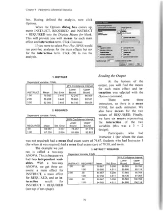
90. Chapter6 ParametricInferentialStatistics
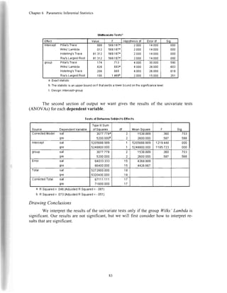
Phrasing ResultsThatAre Significant
If we had received
the following output instead,
we would have had a
significant MANOVA, and
we could statethe following:
a Exatlslalistic
b.Thestausticis anuppsrboundonFhalyisldsa lffisr boundonthesiqnitcancBlml
c.Desi0n:Intercepl+0roup
Ieir oaSrtrocs|alEl. Effoda
Sourca OsoandahlVa.i
Typelllgum
dl xean si0
corected todet sat
gf8
62017.tt8'
963tt att!
2
2
31038.889
13'1t2.222
t.250
9.r65
006
002
htorc€pt Sat
ue
5859605.556
5997338.889
5859605.556
5997338.8S9
I 368.711
I 314.885
000
000
gfoup sal
ore
620tt.t78
863arala
2 31038.089
431t2.222
|.250
9.t65
006
002
Erol sat
0rs
61216 667
6S||6 667
15
15
4281.11',l
1561.,|'rr
T0lal
ote
5985900.000
6152r00000
18
Cor€cled Tolal sal
0re
126291.444
1517611|1 l7
A one-wayMANOVA wascalculatedexaminingtheeffectof training(none,
short-term,long-term)onMZand GREscores.A significanteffectwasfound
(Lambda(4,28)= ,423,p: .014).Follow-upunivariateANOVAs indicated
thatSATscoresweresignificantlyimprovedby training(F(2,15): 7.250,p :
.006).GREscoreswerealsosignificantlyimprovedby training(F(2,15):
9'465,P = '002).
Phrasing ResultsThatAre Not Significant
Theactualexamplepresentedwasnotsignificant.Therefore,wecouldstatethefol-
lowingin theresultssection:
A one-wayMANOVA wascalculatedexaminingtheeffectof training(none,
short-term,or long-term)onSIZ andGREscores.No significanteffectwas
found(Lambda(4,28)= .828,p > .05).NeitherSATnor GREscoreswere
significantlyinfluencedbytraining.
llldbl.Ielrc
Ertscl value d] Frr6t dl Srd
Inlercepl PillaIsTrace
Wilks'Lambda
Holsllln0'sT€cs
RoYsLargsslRoot
.989
.0tI
91.912
91.912
613.592.
6a3.592.
6t3.592.
613.592.
2.000
2.000
2000
2.000
t.000
r.000
1.000
{.000
.000
.000
.000
.000
group piilai's Trec€
Wllks'Lambda
HolellingbTrace
Roy's Largsst Rool
.579
.123
t .350
1 n{o
3.157.
1.t01
't0.t25r
| 000
I 000
I 000
2.000
30.000
28.000
26.000
I 5.000
032
011
008
002
84

91. Chapter7
NonparametricInferentialStatistics
Nonparametrictestsareusedwhenthecorrespondingparametricprocedureis inap-
propriate.Normally,this is becausethe dependentvariable is not interval- or ratio-
scaled.It canalsobebecausethedependentvariableis not normallydistributed.If the
dataof interestarefrequencycounts,nonparametricstatisticsmayalsobeappropriate.
Section7.1 Chi-square Goodnessof Fit
Description
Thechi-squaregoodnessof fit testdetermineswhetheror not sampleproportions
matchthetheoreticalvalues.Forexample,it couldbeusedto determineif adieis"loaded"
or fair.It couldalsobeusedto comparetheproportionof childrenbornwith birthdefects
to the populationvalue(e.g.,to determineif a certainneighborhoodhasa statistically
higher{han-normalrateof birthdefects).
Assumptions
Weneedto makeveryfewassumptions.Therearenoassumptionsabouttheshape
of thedistribution.Theexpectedfrequenciesfor eachcategoryshouldbeatleastl, andno
morethan20%oof thecategoriesshouldhaveexpectedfrequenciesof lessthan5.
SP,S,SData Format
SPSSrequiresonlyasinglevariable.
Runningthe Command
We will createthefollowingdatasetandcall it COINS.sav.The followingdata
representtheflippingof eachof twocoins20times(H iscodedasheads,T astails).
CoiNI: HTH HTHHTH HHTTTHTHTTH
COiN2:TTHHT HTHTTHHTH HTHTHH
Namethetwo variablesCOINI andCOIN2,andcodeH as I andT as2. Thedata
file thatyoucreatewill have20rowsof dataandtwocolumns,calledCOINI andCOIN2.
85

92. Chapter7 NonparametricInferentialStatistics
To run the Chi-Square comman{
click Analyze,thenNonparametricTests,
then Chi-Square. This will bring up the
maindialog box for theChi-SquareTest.
Transferthe variableCOINI into
the Test VariableList. A "fair" coin has
an equal chanceof coming up headsor
tails. Therefore, we will leave the E'"r-
pected Valuessetto All categoriesequal.
We could test a specific set of
proportionsby entering the relative fre-
quencies in the Expected Values area.
Click OK to runtheanalysis.
i E$cOrURutClc '
; 6 Garrna*c
r (. Usarp.dirdrarr0o
l
: :.i)iir'l I
i
i rt,t,i,t I
Reading the Output
The output consistsof two sec-
tions.The first sectiongivesthe frequen-
cies (observed1f) of each value of the
variable.The expectedvalue is given,
alongwith the differenceof the observed
from the expectedvalue (called the re-
sidual).In our example,with 20 flipsof a
coin,we shouldget l0 of eachvalue.
Test Statistics
coinl
unt-uquareo
df
Asymp.Sig.
.200
1
.655
,le*l 1-l RePsts )
:Y,:f Dascri*hrcststistict I
Cdmec lih€nt l
6nsrdlhcir$,lo*l t
Csrd*c t
RiErcrskn ,
d.$dfy I
O*ERadwllon ,
ft.k t
@tkfta 5*b, )
Qudry{onbd }
ROCCtvi,,.
Tail
i Haad
i***- xeio'
.r...X
pKl
n3nI
irydI
3Ll
cotNl
The second section of the
outputgives the resultsof the chi-
squaretest.
a. 0 cells(.0%)haveexpectedfrequencieslessthan
5.Theminimumexpectedcellfrequencyis 10.0.
akrdoprdc* 5unphg.,.
KMgerdant Sffrpbs,,,
2Rddldtudcs",,
KRd*adSsrpbs,,.
Observed
N
Expected
N Residual
Head
Tail
Total
11
9
20
10.0
10.0
1.0
-1.0
86

93. Chapter7 NonparametricInferentialStatistics
Drawing Conclusions
A significantchi-squaretestindicatesthatthedatavaryfromtheexpectedvalues.A testthatisnotsignificaniindicatesthatthedataareconsistentwiththeexpectedvalues.
Phrasing ResultsThatAre Significant
In describingtheresults,youshouldstatethev.alueof chi-square(whosesymbolis1'1'thedegrees.ofdt.aot, it.'rignin.ance level,anaa descriptionof theresults.Forex-ample'with a significantchi-square(for,asample'differentfromtheexampleabove,suchasif wehaduseda "loaded"die),wecourdstatithefoilowing:
A chi-squaregoodnessof fit testwascalculatedcomparingthefrequencyofoccurrenceof eachvalueof a die.It washypothesizedthateachvaluewouldoccuranequalnumberof times.Significanideviationnor trtr rtypothesizedvalueswasfoundfXlSl :25.4g,p i.OS).Thedieappearstobe.,loaded.,,
Notethatthisexampleuseshypotheticalvalues.
Phrasing ResultsThatAre NotSignificant
If theanalysisproducesno significantdifference,asin thepreviousexample,wecouldstatethefollowing:
A chi-squaregoodnessof fit testwascalculatedcomparingthefrequencyofocculrenceof headsandtailsona coin.It washypothesizedthateachvaluewouldoccuran equalnumberof times.No significantdeviationfrom thehypothesizedvalueswasfound(xre): .20,prlOsl. Thecoinapfearsto befair.
Practice Exercise
Use Practice Data Set 2 in Appendix B. In the entire population from which the
sample was drawn , 20yo of employees are clerical, 50Yo are technical, and 30%oare profes-
sional.Determinewhetheror not thesampledrawnconformsto thesevalues.HINT: Enter
therelativeproportionsof thethreesamplesin order(20, 50,30)in the"ExpectedValues"
afea.
Section 7.2 Chi-Square Test of Independence
Description
The chi-squaretest of independencetestswhetheror not two variablesare inde-
pendentof each other. For example,flips of a coin should be independent events, so
knowing the outcomeof one coin tossshouldnot tell us anything aboutthe secondcoin
toss.The chi-squaretestof independenceis essentiallya nonparametricversionof the in-
teraction term in ANOVA.
87

94. Chapter7 NonparametricInferentialStatistics
Drawing Conclusions
A significantchi-squaretest indicatesthat the datavary from the expectedvalues.
A testthat is not significantindicatesthatthedataareconsistentwith the expectedvalues.
Phrosing ResultsThat Are Significant
In describingtheresults,you shouldstatethevalueof chi-square(whosesymbolis
1t;, th" degreesof freedom,the significancelevel,anda descriptionof the results.For ex-
ample,with a significantchi-square(for a sampledifferent from the exampleabove,such
asif we haduseda "loaded"die),we couldstatethefollowing:
A chi-squaregoodnessof fit testwascalculatedcomparingthe frequencyof
occunenceof eachvalueof a die.It washypothesizedthateachvaluewould
occuran equalnumberof times.Significantdeviationfrom the hypothesized
valueswasfoundC6:25.48,p < .05).Thedieappearsto be"loaded."
Notethatthisexampleuseshypotheticalvalues.
Phrasing Results That Are Not Significant
If the analysisproducesno significantdifference,as in the previousexample,we
couldstatethefollowing:
A chi-squaregoodnessof fit testwascalculatedcomparingthe frequencyof
occurrenceof headsand tails on a coin. It was hypothesizedthat eachvalue
would occur an equal numberof times. No significantdeviationfrom the
hypothesizedvalueswasfound(tttl: .20,p > .05).The coin appearsto be
fair.
Practice Exercise
Use PracticeData Set2 in AppendixB. In the entirepopulationfrom which the
samplewas drawn, 20o of employeesareclerical,50Yoaretechnical,and30o/oareprofes-
sional.Determinewhetheror not the sampledrawnconformsto thesevalues.HINT: Enter
therelativeproportionsof thethreesamplesin order(20,50,30) in the"ExpectedValues"
area.
Section7.2 Chi-SquareTestof Independence
Description
The chi-squaretest of independencetestswhetheror not two variablesare inde-
pendentof eachother.For example,flips of a coin shouldbe independentevents,so
knowing the outcomeof one coin tossshouldnot tell us anythingabout the secondcoin
toss.The chi-squaretestof independenceis essentiallya nonparametricversionof the in-
teraction term in ANOVA.
87

95. Chapter7 NonparametricInferentialStatistics
Assumptions
Very few assumptionsareneeded.For example,we makeno assumptionsaboutthe
shapeof the distribution.The expectedfrequenciesfor eachcategoryshouldbe at least l,
andno morethan20o/oof thecategoriesshouldhaveexpectedfrequenciesof lessthan5.
.SP,SSData Format
At leasttwo variablesarerequired.
Running the Command
The chi-squaretest of independenceis a
componentof the Crosstabscommand.For more
details,seethe sectionin Chapter3 on frequency
distributionsfor morethanonevariable.
This exampleusestheCOINS.savexample.
COINI is placedin the Row(s)blank, and COIN2
is placedin the Column(s)blank.
Click Statistics.then check the Chi-
square box. Click Continue.You may also
want to click Cel/s to select expected fre-
quenciesin addition to observedfrequencies,
as we will do on the next page.Click OK to
run the analysis.
llfr}1,* qrg"
Rpports
l.[fltias llllnds* Heb
Compalil&nllt
6nn*rEll."f,rsarMMd
' ConeJat*
Reqn*e$uh
Clarsfy
. OaioRrductlon
Scala
fraqrerrhs,,,
R*lo;,.
P+P{att,,.
*QPlotr,.,
p&ffi |- Cqrddionc
$,iii1ilr'tirir':l
.w.l
H+l
, xire-
i
Or*ut -*-, -
f CedilgacycodlU*r
, il* larna
, [- FiadCrrm#rv : i f- lalar'd
f Llrnbda f Kcnddrldr!
ruTa'rvYY
i lrYa'*o
-Ndridblrttavc -- '. f- [qea
f-Eta , TnFr
- *, f- Uatcru
l- Coc*rgrfs
'ld
l{do}Hlcse6l d.ridbs
'|'.r'' .::'t':,:;, lt-
*:51
.!rd I
siJ
H'bI
88

96. Chapter7 NonparametricInferentialStatistics
ReadingtheOutput
The output consistsof two
parts.The first part givesyou the
counts.In this example,the actual
andexpectedfrequenciesareshown
becausetheywereselectedwith the
Cel/soption.
?r{t$t,,,.l!{h I l?ry1!,,,I
!
Ccrr*c fq.rrt I,--!
;l? 0b*cvcd : Cr"* |
1v rxpccico
fron I
N
P"cc*$or Rrdd'Alc
i
il* npw i if uttlaltddtu I
;l" Colrm I lf $.n*rtu I
t|* ral I ll* n4,a"e*aru*Auco I
1.,..-...-..-..--,..----".*.Ji.-*-..--.--.--.'***--*--***-l
: Nodrlc$aW{t*t -'- ""-"-^ '-"'-"-l
i r no,"u.or"or*r l^ 8o.ndc..trradtr
i
I f Trurlccalcorntr l. Innc*cr*vralrf*
|
I r Xor4.r*rprr
I
COINI' GOIN2Crosstabulatlon
corN2
TotalHead Tail
golNl Fleao uounl
Expected
Count
6.1
4
EN
11
11.0
Tail Count
Expected
Count
4
5.0 4.1
Y
9.0
Total Count
Expected
Count
11
11.0
I
on
20
20.0
Note that you can also use the Cells option to
displaythe percentagesof eachvariablethat areeach
value.This is especiallyusefulwhen your groupsare
differentsizes.
The secondpart of the outputgivesthe results
of thechi-squaretest.The mostcommonlyusedvalue
is the Pearsonchi-square,shown in the first row
(valueof .737).
Chi-SquareTests
Value df
Asymp.Sig
(2-sided)
ExactSig,
(2-sided)
ExactSig.
(1-sided)
PearsonL;nr-!'quare
ContinuityCorrectiorf
LikelihoodRatio
Fisher'sExactTest
Linear-by-Linear
Association
N of ValidCases
{3t"
165
740
700
20
I
1
1
I
.391
.684
.390
.403
.653 .342
a' ComputedonlYfor a 2x2lable
b. 3 cells(75.0%)haveexpectedcountlessthan5. Theminimumexpectedcountis 4.
05.
Drawing Conclusions
A significantchi-squaretestresultindicatesthatthe two variablesarenot inde-
pendent.A valuethatis notsignificantindicatesthatthevariablesdonotvarysignificantly
fromindependence.
89

97. Chapter7 NonparametricInferentialStatistics
Phrasing ResultsThatAre Significant
In describingtheresults,you shouldgivethevalueof chi-square,thedegreesof
freedom,thesignificancelevel,anda descriptionof theresults.For example,with a sig-
nificantchi-square(for a datasetdifferentfromtheonediscussedabove),we couldstate
thefollowing:
A chi-squaretestof independencewascalculatedcomparingthefrequencyof
heartdiseasein menandwomen.A significantinteractionwasfound(f(l) :
23.80,p < .05).Menweremorelikelyto getheartdisease(68%)thanwere
women(40%
Notethatthissummarystatementassumesthatatestwasrunin whichparticipants'sex,as
wellaswhetheror nottheyhadheartdisease,wascoded.
Phrasing ResultsThatAre Not Significant
A chi-squaretestthatis notsignificantindicatesthatthereis nosignificantdepend-
enceof onevariableontheother.Thecoinexampleabovewasnotsignificant.Therefore,
wecouldstatethefollowing:
A chi-squaretest of independencewas calculatedcomparingthe result of
flippingtwo coins.No significantrelationshipwas found(I'(l) = .737,p>
.05).Flipsof acoinappeartobeindependentevents.
Practice Exercise
A researcherwantsto knowwhetheror notindividualsaremorelikelyto helpin an
emergencywhentheyareindoorsthanwhentheyareoutdoors.Of 28 participantswho
wereoutdoors,19helpedand9 didnot.Of 23participantswhowereindoors,8helpedand
15did not.Enterthesedata,andfind out if helpingbehavioris affectedby theenviron-
ment.The key to this problemis in the dataentry.(Hint: How manyparticipantswere
there,andwhatdoyouknowabouteachparticipant?)
Section7.3 Mann-Whitnev UTest
Description
TheMann-WhitneyU testisthenonparametricequivalentof theindependentt test.
It testswhetheror nottwo independentsamplesarefromthesamedistribution.TheMann-
WhitneyU testis weakerthantheindependentt test,andthe/ testshouldbeusedif you
canmeetitsassumptions.
Assumptions
TheMann-WhitneyU testusestherankingsof thedata.Therefore,thedatafor the
two samplesmustbeatleastordinal.Therearenoassumptionsabouttheshapeof thedis-
tribution.
!il;tIFfFF".
90

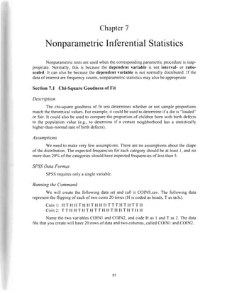
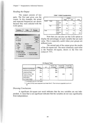
98. Chapter7 NonparametricInferentialStatistics
,SPS,SData Format
Thiscommandrequiresa singlevariablerepresentingthedependentvariableand
asecondvariableindicatinggroupmembership.
Running the Command
This examplewill use a new data
file. It representsl2 participantsin a series
of races.There were long races,medium
races, and short races. Participantseither
had a lot of experience (2), some
experience(l), or no experience(0).
Enter the data from the figure at
right in a new file, and savethe datafile as
RACE.sav. The values for LONG.
MEDIUM, and SHORT represent the
resultsof the race,with I being first place
and12beinglast.
To run the command,click Analyze,thenNon-
parametric Tests, then 2 Independent Samples. This
willbring up themaindialogbox.
Enterthe dependentvariable (LONG, for this
example)in the TestVariableList blank. Enterthe in-
dependentvariable (EXPERIENCE)as the Grouping
Variable.Make surethatMann-WhitneyU is checked.
Click DefineGroupsto selectwhich two groups
you will compare.For this example,we will compare
thoserunnerswith no experience(0) to those runners
with a lot of experience(2). Click OK to run the
analvsis.
iTod Tiryc**-
il7 Mxn.dWn6yu I_ Ko&nonsov'SrnirnovZ
I
l- Mosasa<tcnproactkmc l- W#.Wdrowfrznnrg
I Andy* qaphr U*lx
i R.po.ti ,
I Doroht*o1raru.r ,
Cd||olaaMcrfE t
| 6onralthccl'lodd I
j C*ru|*c )
r Rooa!33hn
'
i cta*iry )
j DatrRoddton )
' Sada )
:@e@J llrsSarfr t
I Q.s*y Cr*rd t
I BOCCuv.,,,
O$squr.,..
thd|*rl...
Rur...
1-sdTpbX-5,..
rl@ttsstpht,.,
eRlnand5{ndnr,,,
KRdetcdsrmplo*.,,
nl 3
nl
'
ei--'
---
n]' rf
bl 2:
liiiriil',,,-5J
IKJ
],TYTI
fry* |
l*J
WMw lbb
[6 gl*l
| &r*!r*l
C.,"* |
ryl
GnuphgVadadr:
fffii0?r-*
l ; ..' ,''r 1,
9l

99. Chapter7 NonparametricInferentialStatistics
Readingthe Output
The outputconsistsof two
sections.The first sectiongivesde-
scriptivestatisticsfor thetwo sam-
ples.Becausethe dataareonly re-
quiredto beordinal, summariesre-
latingto theirranksareused.Those Test Statisticsb
lono
Mann-wnrrneyu
WilcoxonW
z
Asymp.Sig.(2-tailed)
ExactSig.[2'(1-tailed
sis.)l
.000
10.000
-2.309
.021
a
.029
a. Notcorrectedforties.
b.GroupingVariable:experience
Drawing Conclusions
A significantMann-WhitneyU resultindicatesthatthetwo samplesaredifferentin
termsof theiraverageranks.
Phrasing ResultsThatAre Significant
Ourexampleaboveissignificant,sowecouldstatethefollowing:
A Mann-WhitneyUtestwascalculatedexaminingtheplacethatrunnerswith
varyinglevelsof experiencetookin a long-distancerace.Runnerswith no
experiencedidsignificantlyworse(m place: 6.50)thanrunnerswitha lot of
experience(mplace: 2.5A;U = 0.00,p < .05).
Phrasing ResultsThatAre Not Significant
If we conducttheanalysison theshort-distanceraceinsteadof the long-distance
race,wewill getthefollowingresults,whicharenotsignificant.
participantswho had no experienceaveraged6.5 as
theirplacein therace.Thoseparticipantswith a lot of
experienceaveraged2.5astheirplacein therace.
Thesecondsectionof theoutputis theresultof
the Mann-WhitneyU test itself.The valueobtained
was0.0,withasignificancelevelof .021.
Ranks
exDerience N MeanRank SumofRanks
short .00
2.00
Total
4
4
I
4.63
4.38
18.50
17.50
T..t St tlttlct
shorl
Manrr-wtltnoy u
Wilcoxon W
z
Asymp. Sig. (2-tail6d)
ExactSig.[2'(1-tailed
sis.)l
/.cuu
17.500
-.145
.885
t
.886
a. Not corscled for ties.
b GrouprngVanabb: sxporience
Ranks
exDenence N MeanRank Sumof Ranks
rong .uu
2.OO
Total
4
4
8
o.cu
2.50
Zb.UU
10.00
92

100. Chapter7 NonparametricInferentialStatistics
Therefore,we couldstatethe following:
A Mann-Whitney U test was used to examine the difference in the race
performance of runners with no experience and runners with a lot of
experiencein a short-distancerace.No significantdifferencein the resultsof
theracewasfound(U :7.50,p > .05).Runnerswith no experienceaveraged
a placeof 4.63.Runnerswith a lot of experienceaveraged4.38.
Practice Exercise
Assumethatthe mathematicsscoresin PracticeExerciseI (Appendix B) aremeas-
uredon an ordinal scale.Determineif youngerparticipants(< 26) havesignificantlylower
mathematicsscoresthanolderparticipants.
Section7.4 Wilcoxon Test
Description
TheWilcoxontestis thenonparametricequivalentof thepaired-samples(depend-
ent)t test.It testswhetheror nottwo relatedsamplesarefromthesamedistribution.The
Wilcoxontestis weakerthantheindependentI test,sotheI testshouldbeusedif youcan
meetitsassumptions.
Assumptions
TheWilcoxontestisbasedonthedifferencein rankings.Thedatafor thetwosam-
plesmustbeatleastordinal.Therearenoassumptionsabouttheshapeof thedistribution.
SP^SSData Format
Thetestrequirestwo variables.Onevariablerepresentsthedependentvariableat
onelevelof theindependentvariable.Theothervariablerepresentsthedependentvari-
ableatthesecondlevelof theindependentvariable.
Runningthe Command
lrnil$ re*|r u*t
Locatethe commandby clicking Analyze,then Non-
parametric Tests,then 2 RelatedSamples.This exampleuses
theRACE.savdataset.
Crrd*!
'.;,'{'
;l ; --f---"" This will
sd*
bringup thedia-
o*sqr'.., ' I log box for the
*!!fd... I rrr:t^^-.^
ffi | wilcoxon test.
9$l
,Hrl
m-35+- li*.1;X.**"..I Notethesimilar-
-.lggg*g,lggj=l
itv hetween it and
i ; .W tne dialog box
for the dependentt test. If you have trouble,
referto Section6.4on thedependent(paired-
samples)I testin Chapter6.
93
lcucf8drcdom- - " -"-l f l.dltf. --- - --- *
ivti*r, : ip ulte!
'-
sip l- xrNdil :
, Vrnra2 , I
oetm..I

101. Chapter7 NonparametricInferentialStatistics
TransferthevariablesLONGandMEDIUM asa pairandclick OK to runthetest.
This will determineif the runnersperformequivalentlyon long- andmedium-distance
races.
Readingthe Output
Theoutputconsistsof twoparts.Thefirstpartgivessummarystatisticsfor thetwo
variables.Thesecondsectioncontainstheresultof theWilcoxontest(givenas4.
Ranks
N
Mean
Rank
Sumof
Ranks
MEUTUM- NegaUVe
LONG Ranks
Positive
Ranks
Ties
Total
a
4
D
5
3c
12
5.38
4.70
21.50
23.50
TestStatisticsb
A.MEDIUM< LONG
b. tr,lgOtUtr,it>LONG
c.LONG= MEDIUM
Theexampleaboveshowsthatno significantdifferencewasfoundbetweenthere-
sultsof thelong-distanceandmedium-distanceraces.
Phrasing ResultsThatAre Significant
A significantresultmeansthata changehasoccurredbetweenthetwo measure-
ments.If thathappened,wecouldstatethefollowing:
A Wilcoxontestexaminedthe resultsof the medium-distanceand long-
distanceraces.A significantdifferencewasfoundin theresults(Z = 3.40,p <
.05).Medium-distanceresultswerebetterthanlong-distanceresults.
Notethattheseresultsarefictitious.
Phrasing ResultsThatAre Not Significant
In fact,theresultsin theexampleabovewerenotsignificant,sowecouldstatethe
following:
A Wilcoxon test examinedthe resultsof the medium-distanceand long-
distanceraces.No significantdifferencewasfoundin theresults(Z:4.121,
p > .05).Medium-distanceresultswerenotsignificantlydifferentfromlong-
distanceresults.
Practice Exercise
Usethe RACE.savdatafile to determinewhetheror not the outcomeof short-
distanceracesisdifferentfromthatof medium-distanceraces.Phraseyourresults.
MEDIUM -
LONG
z
Asymp.
sig.
(2-tailed)
-1214
.904
a' Basedon
negativeranks.
b'wilcoxon
SignedRanks
Test
94

102. Chapter7 NonparametricInferentialStatistics
Section7.5 Kruskal-WallisIl Test
Description
The Kruskal-Wallis .F/ test is the nonparametricequivalent of the one-way
ANOVA. It testswhetheror not severalindependentsamplescomefrom the samepopula-
tion.
Assumptions
Becausethe test is nonparametric,thereare very few assumptions.However, the
testdoesassumean ordinal levelof measurementfor the dependentvariable. The inde-
pendentvariable shouldbe nominal or ordinal.
,SPS,SData Format
SPSSrequiresonevariableto representthedependentvariable andanotherto rep-
resentthelevelsof theindependentvariable.
Running the Command
This exampleusestheRACE.savdatafile. To run
the command,click Analyze,thenNonparametricTests,
thenK IndependentSamples.This will bring up the main
dialogbox.
Enterthe independentvariable (EXPERIENCE)
asthe Grouping Variable,andclick DefineRangeto de-
fine the lowest(0) and highest(2) values.Enterthe de-
pendent variable (LONG) in the TestVariableList, and
click OK.
Reading the Output
The output consistsof two parts.
The first part gives summarystatisticsfor
eachof the groups definedby the group-
ing (independent)variable.
2
(nC*dsdd.r.,,
RangpforEm{*tEVrri*lt
Mi{run l0
Mrrdlrrrn la
ffi
('$5*|..,.
ffudd,,.
RrJf.,.
l-Samda(-5.,.
tc"{h.I
+ry{|
Hdp I
Co,rpftlbfF )
| 6;?Cl"tsilodd r
i Canl*t I
i Ratatdan
'
;d#rt
I 0d! ildrdoft I
i scdi I
l@J thr Sarbr l
) qr.nr(o.*rd t
I nOCArs,.,
Ranks
exoerience N MeanRank
rong .uu
1.00
2.00
Total
4
4
4
12
10.50
6.50
2.50
95

103. TestStatisticf,b
lonq
unr-uquare
df
Asymp.Sig.
9.846
2
.007
a' KruskalWallisTest
b. GroupingVariable:experience
Drawing Conclusions
Like the one-wayANOVA, the Kruskal-Wallistestassumesthat the groupsare
equal.Thus,a significantresultindicatesthatatleastoneof thegroupsis differentfromat
leastoneothergroup.UnliketheOne-llayANOVAcommand,however,thereareno op-
tionsavailablefor post-hocanalysis.
Phrasing ResultsThatAre Significant
Theexampleaboveis significant,sowecouldstatethefollowing:
A Kruskal-Wallistestwas conductedcomparingthe outcomeof a long-
distanceracefor nmnerswith varyinglevelsof experience.A significant
resultwasfound(H(2): 9.85,p < .01),indicatingthatthegroupsdiffered
fromeachother.Runnerswithnoexperienceaveragedaplacementof 10.50,
whilerunnerswith someexperienceaveraged6.50andrunnerswith a lot of
experienceaveraged2.50.Themoreexperiencethe runnershad,the better
theyperformed.
Phrasing ResultsThqtAre Not Significant
If we conductedtheanalysisusingtheresultsof theshort-distancerace,wewould
getthefollowingoutput,whichisnotsignificant.
Chapter7 NonparametricInferentialStatistics
The secondpartof theoutputgivestheresults
of theKruskal-Wallistest(givenasa chi-squarevalue,
butwe will describeit asan II).The examplehereis a
significantvalueof 9.846.
Ranks
exoenence N MeanRank
snon .uu
1.00
2.00
Total
4
4
4
12
6.3E
7.25
5.88
Teet Statlstlc$'b
short
unFuquare
df
Asymp.Sig.
.299
2
.861
a. KruskalWallisTest
b.GroupingVariable:experience
Thisresultisnotsignificant,sowecouldstatethefollowing:
A Kruskal-Wallistest was conductedcomparingthe outcomeof a short-
distanceracefor runnerswith varyinglevelsof experience.No significant
differencewasfound(H(2):0.299,p > .05),indicatingthatthegroupsdid
notdiffersignificantlyfromeachother.Runnerswith noexperienceaveraged
a placementof 6.38,whilenmnerswith someexperienceaveraged7.25and
nmnerswith a lot of experienceaveraged5.88.Experiencedid not seemto
influencetheresultsof theshort-distancerace.
96

104. Chapter7 NonparametricInfbrentialStatistics
Practice Exercise
UsePracticeDataSet2 in AppendixB. Jobclassificationis ordinal (clerical<
technical< professional).Determineif malesandfemaleshavedifferinglevelsofjob clas-
sifications.Phraseyourresults.
Section7.6 Friedman Test
Description
TheFriedmantestis thenonparametricequivalentof a one-wayrepeated-measures
ANOVA. It isusedwhenyouhavemorethantwomeasurementsfromrelatedparticipants.
Assumptions
Thetestusestherankingsof thevariables,sothedatamustbeat leastordinal.No
otherassumptionsarerequired.
SP,SSData Format
SPSSrequiresat leastthreevariablesin the SPSSdatafile. Eachvariablerepre-
sentsthedependentvariableatoneof thelevelsof theindependentvariable.
Runningthe Command
Locatethecommandby clickingAnalyze,then
NonparametricTests,thenK RelatedSamples.Thiswill
bringupthemaindialogbox.
f r;'ld{iv f* Cdi#ln
Placeall thevariablesrepresentingthelevelsof theindependentvariablein the
TestVariablesarea.Forthisexample,usetheRACE.savdatafile andthevariablesLONG,
MEDIUM.andSHORT.ClickO1(.
97

105. Chapter7 NonparametricInferentialStatistics
ReadingtheOutput
Theoutputconsistsof two sections.Thefirstsectiongivesyousummarystatistics
for eachof thevariables.Thesecondsectionof theoutputgivesyoutheresultsof thetest
as a chi-squarevalue.The exampleherehasa valueof 0.049and is not significant
(Asymp.Sig.,otherwiseknownasp,is.976,whichisgreaterthan.05).
Ranks TestStatisticf
Mean
Rank
LUNU
MEDIUM
SHORT
2.00
2.04
1.96
12
Chi-Square| .049
dflz
Asymp.Sis.
| .976
a. FriedmanTest
Drawing Conclusions
The Friedmantestassumesthatthethreevariablesarefrom the samepopulation.A
significantvalueindicatesthatthevariablesarenot equivalent.
PhrasingResultsThatAreSignificant
If we obtaineda significantresult,we could statethe following (theseare hypo-
theticalresults):
A Friedmantest was conductedcomparingthe averageplace in a race of
nrnnersfor short-distance,medium-distance,and long-distanceraces.A sig-
nificantdifferencewas foundC@: 0.057,p < .05).The lengthof the race
significantlyaffectstheresultsof therace.
PhrasingResultsThatAreNotSignificant
In fact,theexampleabovewasnotsignificant,sowecouldstatethefollowing:
A Friedmantestwasconductedcomparingthe averageplacein a raceof
runnersfor short-distance,medium-distance,and long-distanceraces.No
significantdifferencewasfounddg = 0.049,p > .05).Thelengthof the
racedidnotsignificantlyaffecttheresultsof therace.
Practice Exercise
Usethedatain PracticeDataSet3 in AppendixB. If anxietyis measuredonanor-
dinal scale,determineif anxietylevelschangedovertime.Phraseyourresults.
98

106. $
't,s
i$
.fi
j
Chapter8
TestConstruction
Section 8.1 ltem-Total Analvsis
Description
Item-totalanalysisis a way to assessthe internal consistencyof a dataset.As
such,it is oneof manytestsof reliability. Item-totalanalysiscomprisesa numberof items
thatmakeup a scaleor testdesignedto measurea singleconstruct(e.g.,intelligence),and
determinesthe degreeto which all of the itemsmeasurethe sameconstruct.It doesnot tell
you if it is measuringthe correctconstruct(thatis a questionof validity). Beforea testcan
bevalid,however,it mustfirstbereliable.
Assumptions
All theitemsin thescaleshouldbemeasuredon an interval or ratio scale.In addi-
tion,eachitem shouldbe normallydistributed.If your itemsareordinal in nature,you can
conductthe analysisusing the Spearmanrho correlationinsteadof the Pearsonr correla-
tion.
SP.SSData Forrnat
SPSSrequiresone variablefor eachitem (or
question)in the scale.In addition,you must havea
variablerepresentingthetotal scorefor the scale.
iilrliililrr'
.q! l
I"1l
J13l
.ry1
|7 nagris{icsitqorrcldimr
click OK. (For morehelp on conductingconelations,
culatedwith thetechniquesdiscussedin Chapter2.
, CondationCoalfubr*c
l|7 P"as* l- Kcndafsta* f- Spoamm
l**-*__.-_^__
, Tsd ot SlJnific&cs
'.
I rr r'oorxaa f ona.{atud I
I Andyle Grrphs Ulilities Window Help
RPpo*s
, Ds$rripllvoStatirlicc )
Ccmpar*Msans F
GtneralLinearMadel I
WRiqression )
!:*l',." :
Conducting the Test
Item-totalanalysisusesthe
Pearson Coruelation command.
To conduct it, open the
QUESTIONS.savdatafile you cre-
ated in Chapter2. Click Analyze,
thenCoruelate,thenBivariate.
Placeall questionsand the
total in the right-handwindow, and
seeChapter5.) The totalcanbe cal-
Vuiabla*
99

107. Chapter8 TestConstruction
ReadingtheOutput
The output consistsof a
correlationmatrix containingall
questionsand the total. Use the
columnlabeledTOTAL, and lo-
cate the correlationbetweenthe
total scoreand eachquestion.In
the exampleat right, QuestionI
hasa correlationof 0.873with the
totalscore.Question2 hasacorre-
lation of -0.130 with the total.
Question3 has a correlationof
0.926withthetotal.
Correlatlons
o1 o2 Q3 TOTAL
Lll l'oarson,orrelallon
Sig.(2-tailed)
N
1.000
4
cll
.553
4
t to
.282
4
o/J
.127
4
UZ PearsonCorrelalion
Si9.(2-tailed)
N
-.447
.553
4
1.000
4
-.229
.771
4
-.130
.870
4
Q3 P€arsonCorrelation
Sig.(2-tailed)
N
.718
.?82
4
..229
.771
4
1.000
4
.YZO
.074
4
TOTAL PearsonConelation
Sig.(2-tailed)
N
.873
.127
4
-.130
.870
4
.926
.074
4
1.000
4
Interpreting the Output
Item-totalcorrelationsshouldalwaysbepositive.If youobtaina negativecorrela-
tion, that questionshouldbe removedfrom the scale(or you may considerwhetherit
shouldbereverse-keyed).
Generally,item-totalcorrelationsof greaterthan 0.7 areconsidereddesirable.
Thoseof lessthan0.3areconsideredweak.Any questionswith correlationsof lessthan
0.3shouldberemovedfromthescale.
Normally,theworstquestionisremoved,thenthetotalisrecalculated.Aftertheto-
tal is recalculated,the item-totalanalysisis repeatedwithoutthe questionthat wasre-
moved.Then,if anyquestionshavecorrelationsof lessthan0.3,theworstoneis removed,
andtheprocessisrepeated.
Whenall remainingcorrelationsaregreaterthan0.3,the remainingitemsin the
scaleareconsideredtobethosethatareinternallyconsistent.
Section8.2 Cronbach'sAlpha
Description
Cronbach'salphais a measureof internalconsistency.As such,it is oneof many
testsof reliability. Cronbach'salphacomprisesa numberof itemsthatmakeup a scale
designedto measurea singleconstruct(e.g.,intelligence),anddeterminesthe degreeto
whichall theitemsaremeasuringthesameconstruct.It doesnottell youif it is measuring
thecorrectconstruct(thatis a questionof validity).Beforea testcanbevalid,however,it
mustfirstbereliable.
Assumptions
All theitemsin thescaleshouldbemeasuredonanintervalor ratio scale.In addi-
tion,eachitemshouldbenormallydistributed.
100

108. Chapter8 TestConstruction
,SP,SSData Format
SPSSrequiresonevariablefor eachitem(orquestion)in thescale.
Runningthe Command
This example uses the QUEST-
IONS.savdatafile we firstcreatedin Chapter
2. Click Analyze,thenScale,thenReliability
Analysis.
Thiswill bringupthemaindialogbox
for Reliability Analysis.Transferthe ques-
tionsfrom your scaleto theItemsblank,and
click OK.Do nottransferanyvariablesrepre'
sentingtotalscores.
ReadingtheOutput
In this example,the reliabilitycoefficientis 0.407.
Numberscloseto 1.00areverygood,but numberscloseto
0.00representpoorinternalconsistency.
Section8.3 Test-RetestReliability
Udtbr Wh&* tbb
)
f:
;
l,
it.
)
)
NotethatwhenyouchangetheoP-
tionsunderModel,additionalmeasuresof
internalconsistency(e.9.,split-half)can
becalculated.
RelLrltilityStntistics
Cronbach's
Aloha N ofltems
.407 3
Description
Test-retestreliabilityis a measureof temporalstability.As such,it is a measure
of reliability.Unlikemeasuresof internalconsistencythattell youtheextentto whichall
of thequestionsthatmakeup a scalemeasurethesameconstruct,measuresof temporal
stabilitytellyouwhetheror nottheinstrumentisconsistentovertimeand/orovermultiple
administrations.
Assumptions
Thetotalscorefor thescaleshouldbeanintervalor ratio scale.Thescalescores
shouldbenormallydistributed.
ql
*
q3
l0l

109. Chapter8 TestConstruction
.SP,S,SData Format
SPSSrequiresavariablerepresentingthetotalscorefor thescaleatthetimeof first
administration.A secondvariablerepresentingthetotalscorefor thesameparticipantsata
differenttime(normallytwoweekslater)isalsorequired.
Runningthe Command
Thetest-retestreliabilitycoefficientis simplya Pearsoncorrelationcoefficientfor
therelationshipbetweenthetotalscoresfor thetwo administrations.To computethecoef-
ficient,follow thedirectionsfor computinga Pearsoncorrelationcoefficient(Chapter5,
Section5.1).Usethetwovariablesrepresentingthetwoadministrationsof thetest.
Readingthe Output
The correlationbetweenthetwo scoresis thetest-retestreliabilitycoeffrcient.It
shouldbepositive.Strongreliability is indicatedby valuescloseto 1.00.Weakreliability
isindicatedby valuescloseto0.00.
Section8.4 Criterion-Related Validitv
Description
Criterion-relatedvaliditydeterminestheextentto whichthescaleyou aretesting
correlateswith a criterion.Forexample,ACTscoresshouldcorrelatehighlywith GPA.If
theydo,thatisa measureof validity forACTscores.If theydonot,thatindicatesthatACT
scoresmaynotbevalidfor theintendedpurpose.
Assumptions
All of thesameassumptionsfor thePearsoncorrelationcoefficientapplyto meas-
uresof criterion-relatedvalidity(intervalor ratio scales,normaldistribution,etc.).
.SP,S,SData Format
Two variablesarerequired.Onevariablerepresentsthetotalscorefor thescaleyou
aretesting.Theotherrepresentsthecriterionyouaretestingit against.
Runningthe Command
Calculatingcriterion-relatedvalidityinvolvesdeterminingthePearsoncorrelation
valuebetweenthescaleandthecriterion.SeeChapter5,Section5.1for completeinforma-
tion.
ReadingtheOutput
Thecorrelationbetweenthetwo scoresis thecriterion-relatedvaliditycoefficient.
It shouldbepositive.Strongvalidity is indicatedby valuescloseto 1.00.Weakvalidity is
indicatedbyvaluescloseto0.00.
102

110. AppendixA
EffectSize
Many disciplinesare placing increasedemphasison reporting effect size. While
statisticalhypothesistestingprovidesa way to tell the oddsthat differencesarereal,effect
sizesprovide a way to judge the relativeimportanceof thosedifferences.That is, they tell
us thesizeof thedifferenceor relationship.They arealsocriticalif you would like to esti-
matenecessarysamplesizes,conducta poweranalysis,or conducta meta-analysis.Many
professionalorganizations(e.g.,the AmericanPsychologicalAssociation)arenow requir-
ing or stronglysuggestingthateffectsizesbe reportedin additionto the resultsof hypothe-
sistests.
Becausethereare at least4l different typesof effect sizes,reachwith somewhat
differentproperties,the purposeof this Appendix is not to be a comprehensiveresourceon
effect size,but ratherto showyou how to calculatesomeof the mostcommonmeasuresof
effectsizeusingSPSS15.0.
Cohen's d
One of the simplestand most popular measuresof effect size is Cohen's d.
Cohen'sd is a memberof a classof measurementscalled"standardizedmeandifferences."
In essence,d is thedifferencebetweenthetwo meansdividedby theoverallstandard de-
viation.
It is not only a popularmeasureof effectsize,but Cohenhasalsosuggesteda sim-
ple basisto interpretthevalueobtained.Cohen'suggestedthateffectsizesof .2 aresmall,
.5aremedium,and.8arelarge.
We will discussCohen's d asthepreferredmeasureof effect sizefor I tests.Unfor-
tunately,SPSSdoesnot calculateCohen's d. However,this appendixwill coverhow to
calculateit from the outputthatSPSSdoesproduce.
EffectSizeforSingle-Samplet Tests
AlthoughSPSSdoesnot calculateeffectsizefor the single-sample/ test,calculat-
ing Cohen'sd is a simplematter.
' Kirk, R.E. (1996). Practicalsignificance:A conceptwhosetime has come.Educational& Psychological
Measurement,56, 746-759.
' Cohen,J. (1992).A powerprimer.PsychologicalBulletin, t t 2, 155-159.
103

111. Om'S$da sltb.tr
xoan
std
Dflalon
Std Eror
Ygan
LENOIH 0 16 qnnn | 9?2
AppendixA Effect Size
T-Test
o'r..Srt!- Iad
TsstValuo= 35
d
slg
(2-lailsd)
Igan
Dill6f6nao
95$ Conld6nca
lhlld.t ottho
uo00r
71r' I sooo I l55F-07
Cohen's d for a single-sampleI testis equal
to the mean differenceover the standard de-
viation. If SPSSprovidesus with the follow-
ing output,we calculated asindicatedhere:
t.t972
d =.752
D
sD
.90
d-
d-
In this example,using Cohen's guidelinesto judge effect size,we would have an effect
sizebetweenmediumandlarge.
EffectSizefor Independent-Samplest Tests
Calculatingeffectsizefromtheindependentt testoutputisa littlemorecomplex
becauseSPSSdoesnot provideus with thepootedstandarddeviation.The uppersection
of the output,however,doesprovideus with the informationwe needto calculateit. The
outputpresentedhereis thesameoutputwe workedwith in Chapter6.
Group Statlltlcr
morntno N Mean Std. Oeviation
Std.Error
Mean
graoe No
yes
z
2
UZ.SUUU
78.0000
J.JJIDJ
7.07107
Z,SUUUU
s.00000
S pooled
=
(n,-1)s,2+(n, -l)sr2
nr+nr-2
/12- tlr.Sr552+(2-t)7.07| (
rpooted-
2+21
S pool"d
=
Spooted
= 5'59
Oncewe havecalculatedthe pooledstandard deviation(spooud),we cancalculate
Cohen'sd.
, x,-x,Q=--
S pooled
, 82.50- 78.00
o =-
5.59
d =.80
104

112. AppendixA Effect Size
So, in this example,using Cohen'sguidelinesfor the interpretationof d, we would have
obtaineda largeeffectsize.
EffectSizeforPaired-Samplest Tests
As you have probably learnedin your statisticsclass,a paired-samplesI test is
reallyjust a specialcaseof the single-sampleI test.Therefore,the procedurefor calculat-
ing Cohen'sd is alsothe same.The SPSSoutput,however,looksa little different,soyou
will betakingyour valuesfrom differentareas.
Pair€dSamplosTest
PairedDifferences
df
sig
(2-tailed)Mean
std.
f)eviatior
Std.Error
Mean
95% Confidence
Intervalof the
f)iffcrcnne
Lower Upper
YAlt 1 |'KE ttss I
. FINAL -22.809s A OTqA 1.9586 -26.8952 -18.7239 11.646 20 .000
,Du --
JD
-22.8095
8.9756
d = 2.54
Notice that in this example,we representthe effect size (d; as a positive number
eventhoughit is negative.Effectsizesarealwayspositivenumbers.In thisexample,using
Cohen'sguidelinesfor the interpretationof d, we havefounda very largeeffect size.
12(Coefficient of Determination)
While Cohen's d is the appropriatemeasureof effect size for / tests,correlation
and regressioneffect sizesshouldbe determinedby squaringthe correlationcoefficient.
This squaredcorrelationis calledthecoefficientof determination. Cohen' suggestedhere
thatcorrelationsof .5, .3,and.l correspondedto large,moderate,andsmallrelationships.
Thosevaluessquaredyield coefficientsof determinationof .25,.09,and.01respectively.
It would appear,therefore,that Cohenis suggestingthat accountingfor 25o/oof the vari-
ability representsa largeeffbct,9oha moderateeffect,andlo/oa smalleffect.
EffectSizefor Correlation
Nowhere is the effect of samplesize on statisticalpower (and thereforesignifi-
cance)moreapparentthanwith correlations.Given a largeenoughsample,any correlation
canbecomesignificant.Thus,effect sizebecomescritically importantin the interpretation
of correlations.
'Cohen, J. (1988). Statisticalpower analysisfor the behavioralsciences(2"ded). New Jersey:Lawrence
Erlbaum.
105

113. AppendixA Effect Size
The standardmeasureof effect sizefor correlationsis the coefficient of determi-
nation (r2) discussedabove.The coefficient should be interpretedas the proportion of
variance in the dependentvariable that canbe accountedfor by the relationshipbetween
theindependentanddependentvariables.While Cohenprovidedsomeusefulguidelines
for interpretation,eachproblemshouldbe interpretedin termsof its true practicalsignifi-
cance.For example,if a treatmentis very expensiveto implement,or hassignificantside
effects,then a largercorrelationshouldbe requiredbeforethe relationshipbecomes"im-
portant."For treatmentsthat arevery inexpensive,a much smallercorrelationcan be con-
sidered"important."
To calculatethe coefficientof determination,simply takethe r valuethat SPSS
providesandsquareit.
EffectSizefor Regression
TheModelSummarysec-
tion of the output reportsR2 for
you. The example output here
showsa coefficient of determi-
nation of .649,meaningthat al-
most65% (.649of the variabil-
ity in the dependentvariable is
accountedfor by the relationship
betweenthe dependentand in-
dependentvariables.
EtaSquaredQtz)
A third measureof effect sizeis Eta Squared(ry2).Eta Squared is usedfor Analy-
sisof Variancemodels.The GLM (GeneralLinearModel) functionin SPSS(the function
thatrunsthe proceduresunderAnalyze-General Linear Model) will provideEta Squared
(tt').
Eta Squaredhasan interpretationsimilarto a squaredcor-
relationcoefficient1l1.lt representstheproportionof thevariance n, -
SS"ik",
accountedfor by the effect.-Unlike ,2, ho*euer, which represents
tt -
Sqr," . SS*
onlylinearrelationships,,72canrepresentanytypeofrelationship.
EffectSizefor Analysisof Variance
For mostAnalysisof Varianceproblems,you shouldelectto reportEta Squared
asyoureffectsizemeasure.SPSSprovidesthiscalculationfor youaspartof theGeneral
LinearModel(GLIrl)command.
To obtainEta Squared,yousimplyclickon theOptionsbox in themaindialog
box for theGLM commandyouarerunning(thisworksfor Univariate,Multivariate,and
RepeatedMeasuresversionsof thecommandeventhoughonly the Univariateoptionis
presentedhere).
ModelSummary
Model R RSouare
Adjusted
R Souare
Std.Error
of the
Estimate
.8064 .649 .624 16.1480
a. Predictors:(Constant),HEIGHT
106

114. Appendix A Effect Size
Onceyou haveselectedOptions,a new
dialog box will appear.Oneof the optionsin
that box will beEstimatesof ffict sze. When
you selectthat box, SPSSwill provideEta
Squaredvaluesaspartofyour output.
l-[qoral*
|- $FdYr|dg
f A!.|it?ld
rli*dr
f'9n drffat*l
Cr**l.|tniliivdrra5:
TestsotEetweerF$iltectsEftcct3
tl l c,,*| n* |
DependenlVariable:score
Source
TypelllSum
nf Sdila!es df tean Souare F siq,
PadialEta
Souared
u0rrecleoM00el
Inlercepl
gr0up
Enor
Total
CorrectedTotal
10.450r
91.622
10.450
3.283
105.000
13.733
2
4
I
1
12
15
't4
5.225
s't.622
5.225
.274
19.096
331.862
1S.096
.000
.000
.000
761
965
761
a.RSquared= .761(AdiusiedRSquared= .721)
In theexamplehere,we obtainedanEta Squaredof .761for our maineffectfor
groupmembership.Becausewe interpretEta Squaredusingthesameguidelinesas,', we
wouldconcludethatthisrepresentsalargeeffectsizefor groupmembership.
107

116. Appendix B PracticeExerciseDataSets
PracticeDataSet2
A surveyof employeesis conducted.Eachemployeeprovidesthe following infor-
mation: Salary (SALARY), Years of Service (YOS), Sex (SEX), Job Classification
(CLASSIFY),andEducationLevel(EDUC).Notethatyou will haveto codeSEX (Male:
l, Female: 2) andCLASSIFY (Clerical: l, Technical: 2, Professional: 3).
ll*t:g - Jrs$q
Numsric
lNumedc
SALARY
35,000
18,000
20,000
50,000
38,000
20,000
75,000
40,000
30,000
22,000
23,000
45,000
YOS SEX
8 Male
4 Female
I Male
20 Female
6 Male
6 Female
17 Male
4 Female
8 Male
l5 Female
16 Male
2 Female
CLASSIFY EDUC
Technical 14
Clerical l0
Professional l6
Professional l6
Professional 20
Clerical 12
Professional 20
Technical 12
Technical 14
Clerical 12
Clerical 12
Professional l6
PracticeDataSet3
Participantswho havephobiasaregivenoneof threetreatments(CONDITION).
Theiranxietylevel(1 to l0) is measuredatthreeintervals-beforetreatment(ANXPRE),
onehour aftertreatment(ANXIHR), andagainfour hoursaftertreatment(ANX4HR).
Notethatyouwill haveto codethevariableCONDITION.
4lcondil ,Numeric
7l i'- '* '"
ll0

117. Appendix B PracticeExerciseData Sets
ANXPRE
8
t0
9
7
7
9
l0
9
8
6
8
6
9
l0
7
ANXIHR
7
l0
7
6
7
4
6
5
3
3
5
5
8
9
6
CONDITION
Placebo
Placebo
Placebo
Placebo
Placebo
ValiumrM
ValiumrM
ValiumrM
ValiumrM
ValiumrM
ExperimentalDrug
ExperimentalDrug
ExperimentalDrug
ExperimentalDrug
ExperimentalDrug
ANX4HR
7
l0
8
6
7
5
I
5
5
4
3
2
4
4
3
lll

118. AppendixC
Glossary
All Inclusive.A setof eventsthatencompasseseverypossibleoutcome.
Alternative Hypothesis.The oppositeof the null hypothesis,normally showingthat there
is a true difference.Generallv. this is the statementthat the researcherwould like to
support.
CaseProcessingSummary. A sectionof SPSSoutputthat lists the numberof subjects
usedin theanalysis.
Coefficient of Determination. The value of the correlation, squared.It provides the
proportionof varianceaccountedfor by therelationship.
Cohen's d. A common and simplemeasureof effect sizethat standardizesthe difference
betweengroups.
Correlation Matrix. A sectionof SPSSoutput in which correlationcoefficientsare
reportedfor allpairsof variables.
Covariate. A variableknown to be relatedto the dependentvariable,but not treatedasan
independentvariable.Usedin ANCOVA asa statisticalcontroltechnique.
Data Window. The SPSSwindow that containsthe datain a spreadsheetformat. This is
the window usedfor runningmostcommands.
Dependent Variable. An outcome or responsevariable. The dependentvariable is
normallydependenton the independentvariable.
Descriptive Statistics.Statisticalproceduresthatorganizeandsummarizedata.
$ nialog Box. A window that allows you to enter information that SPSSwill use in a
$ command.
t
* OichotomousVariables.Variableswithonlytwolevels(e.g.,gender).
il
I DiscreteVariable.A variablethatcanhaveonly certainvalues(i.e.,valuesbetween
'f *hich thereisnoscore,likeA, B, C,D, F).
I'
i Effect Size.A measurethat allows oneto judge the relativeimportanceof a differenceor
. relationshipby reportingthe sizeof a difference.
Eta Squared(q2).A measureof effectsizeusedin Analysisof Variancemodels.
I 13

119. AppendixC Glossary
Grouping Variable. In SPSS,the variableusedto representgroupmembership.SPSS
often refersto independentvariablesas groupingvariables;SPSSsometimesrefersto
groupingvariablesasindependentvariables.
IndependentEvents.Two eventsareindependentif informationaboutoneeventgivesno
informationaboutthesecondevent(e.g.,twoflipsof acoin).
IndependentVariable.Thevariablewhoselevels(values)determinethegroupto whicha
subjectbelongs.A true independentvariableis manipulatedby the researcher.See
GroupingVariable.
Inferential Statistics.Statisticalproceduresdesignedto allow the researcherto draw
inferencesaboutapopulationonthebasisof asample.
Interaction.With morethanoneindependentvariable,aninteractionoccurswhena level
of oneindependentvariableaffectstheinfluenceof anotherindependentvariable.
Internal Consistency.A reliabilitymeasurethatassessesthe extentto which all of the
itemsin aninstrumentmeasurethesameconstruct.
Interval Scale.A measurementscalewhereitems are placedin mutuallyexclusive
categories,with equal intervalsbetweenvalues.Appropriatetransformationsinclude
counting,sorting,andaddition/subtraction.
Levels.Thevaluesthata variablecanhave.A variablewiththreelevelshasthreepossible
values.
Mean.A measureof centraltendencywherethesumof thedeviationscoresequalszero.
Median.A measureof centraltendencyrepresentingthemiddleof a distributionwhenthe
dataaresortedfromlow tohigh.Fiftypercentof thecasesarebelowthemedian.
Mode. A measureof centraltendencyrepresentingthe value(or values)with the most
subjects(thescorewiththegreatestfrequency).
Mutually Exclusive.Two events are mutually exclusivewhen they cannotoccur
simultaneously.
Nominal Scale.A measurementscalewhereitemsare placedin mutuallyexclusive
categories.Differentiationis by nameonly(e.g.,race,sex).Appropriatecategoriesinclude
"same"or "different." Appropriatetransformationsincludecounting.
NormalDistribution.A symmetric,unimodal,bell-shapedcurve.
Null Hypothesis.The hypothesisto be tested,normally in which there is no tnre
difference.It ismutuallyexclusiveof thealternativehypothesis.
n4

120. AppendixC Glossary
Ordinal Scale. A measurementscale where items are placed in mutually exclusive
categories, in order. Appropriate categories include "same," "less," and "more."
Appropriatetransformationsincludecountingandsorting.
Outliers. Extremescoresin a distribution.Scoresthat arevery distantfrom the meanand
therestof the scoresin the distribution.
Output Window. The SPSSwindow thatcontainstheresultsof an analysis.The left side
summarizesthe resultsin an outline.The right sidecontainstheactualresults.
Percentiles(Percentile Ranks). A relativescorethatgivesthepercentageof subjectswho
scoredat the samevalueor lower.
Pooled Standard Deviation. A singlevaluethat representsthe standarddeviationof two
groupsofscores.
Protected Dependent/ Tests.To preventthe inflation of a Type I error,the level needed
to be significantis reducedwhenmultipletestsareconducted.
Quartiles. The points that define a distribution into four equal parts.The scoresat the
25th,50th,and75thpercentileranks.
Random Assignment.A procedurefor assigningsubjectsto conditionsin which each
subjecthasanequalchanceofbeing assignedto anycondition.
Range.A measureof dispersionrepresentingthe numberof points from the highestscore
throughthe lowestscore.
Ratio Scale. A measurementscale where items are placed in mutually exclusive
categories, with equal intervals between values, and a true zero. Appropriate
transformationsincludecounting,sorting,additiott/subtraction,andmultiplication/division.
Reliability. An indicationof the consistencyof a scale.A reliable scaleis intemally
consistentandstableovertime.
Robust. A testis saidto be robustif it continuesto provideaccurateresultsevenafterthe
violationof someassumptions.
Significance.A differenceis said to be significantif the probability of making a Type I
error is lessthan the acceptedlimit (normally 5%). If a differenceis significant,the null
hypothesisis rejected.
Skew. The extentto which a distributionis not symmetrical.Positiveskewhasoutlierson
thepositive(right)sideof thedistribution.Negativeskewhasoutlierson thenegative(left)
sideof thedistribution.
Standard Deviation. A measureof dispersionrepresentinga special type of average
deviationfrom themean.
I 15

121. AppendixC Glossary
StandardError of Estimate.The equivalentof the standarddeviationfor a regression
line.Thedatapointswill benormallydistributedaroundtheregressionlinewith a standard
deviationequalto thestandarderrorof theestimate.
StandardNormal Distribution.A normaldistributionwith a meanof 0.0anda standard
deviationof 1.0.
StringVariable.A stringvariablecancontainlettersandnumbers.Numericvariablescan
containonlynumbers.MostSPSScommandswill notfunctionwith stringvariables.
Temporal Stability. This is achievedwhenreliabilitymeasureshavedeterminedthat
scoresremainstableovermultipleadministrationsof theinstrument.
Tukey's HSD. A post-hoccomparisonpurportedto revealan "honestlysignificant
difference"(HSD).
Type I Error. A Type I erroroccurswhenthe researchererroneouslyrejectsthe null
hypothesis.
Type II Error. A TypeII erroroccurswhentheresearchererroneouslyfailsto rejectthe
nullhypothesis.
Valid Data.DatathatSPSSwill usein itsanalyses.
Validity.An indicationof theaccuracyof a scale.
Variance.A measureof dispersionequaltothesquaredstandarddeviation.
l16

122. AppendixD
SampleDataFilesUsedin Text
A varietyof smalldatafilesareusedin examplesthroughoutthistext.Hereisa list
of whereeachappears.
COINS.sav
Variables:
Enteredin Chapter7
GRADES.sav
Variables:
Enteredin Chapter6
HEIGHT.sav
Variables:
Enteredin Chapter4
QUESTIONS.Sav
Variables:
Enteredin Chapter2
Modifiedin Chapter2
COINI
COIN2
PRETEST
MIDTERM
FINAL
INSTRUCT
REQUIRED
HEIGHT
WEIGHT
SEX
Ql
Q2(recodedin Chapter2)
Q3
TOTAL (addedin Chapter2)
GROUP(addedin Chapter2)
tt7

123. AppendixD SampleDataFilesUsedin Text
RACE.sav
Variables: SHORT
MEDIUM
LONG
EXPERIENCE
EnteredinChapter7
SAMPLE.sav
Variables: ID
DAY
TIME
MORNING
GRADE
WORK
TRAINING(addedin Chapter1)
Enteredin ChapterI
Modifiedin ChapterI
SAT.sav
Variables: SAT
GRE
GROUP
Enteredin Chapter6
Other Files
Forsomepracticeexercises,seeAppendixB for neededdatasetsthatarenotusedin any
otherexamplesin thetext.
l18

124. r{
ril
AppendixE
Informationfor Users
of EarlierVersionsof SPSS
Therearea numberof differencesbetweenSPSS15.0andearlierversionsof the
software.Fortunately,mostof themhavevery little impacton usersof thistext.In fact,
mostusersof earlierversionswill beableto successfullyusethistextwithoutneedingto
referencethisappendix.
Variable nameswere limited to eight characters.
Versionsof SPSSolderthan12.0arelimitedto eight-charactervariablenames.The
othervariablenamerulesstillapply.If youareusinganolderversionof SPSS,youneedto
makesureyouuseeightor fewerlettersforyourvariablenames.
The Data menu will look different.
The screenshotsin the text where the Data
menuis shownwill look slightly differentif you are
using an older versionof SPSS.Thesemissingor
renamedcommandsdo not have any effect on this
text,but themenusmay look slightly different.
If you are using a versionof SPSSearlier
than 10.0,theAnalyzemenuwill be calledStatistics
instead.
Graphing functions.
Priorto SPSS12.0,thegraphingfunctionsof SPSSwerevery limited.If youare
using a versionof SPSSolder than version12.0,third-partysoftwarelike Excel or
SigmaPlotis recommendedfor theconstructionof graphs.If youareusingVersion14.0of
thesoftware,useAppendixF asanalternativeto Chapter4,whichdiscussesgraphing.
Dsta TlrBfqm rn4aa€ getu t
oe&reoacs,.,
r hertYffd,e
l|]lrffl Clsl*t
GobCse",,
l19

125. Appendix E Informationfor Usersof EarlierVersionsof SPSS
Variableiconsindicatemeasurementtype.
In versionsof SPSSearlier
than 14.0,variableswererepresented
in dialog boxes with their variable
label and an icon that represented
whether the variable was string or
numeric(the examplehereshowsall
variablesthatwerenumeric).
Starting with Version 14.0,
SPSSshows additional information
about eachvariable.Icons now rep-
resentnot only whethera variableis
numericor not, but alsowhat type of
measurementscale it is. Nominal
variablesare representedby the &
icon. Ordinal variables are repre-
sentedby the dfl i.on. Interval and
ratio variables(SPSSrefersto them
as scale variables) are represented
bv the d i"on.
It liqtq'ftc$/droyte
sqFr*u.,|4*r.-r-lqql{.,I
SeveralSPSSdatafilescannowbeopenat once.
Versionsof SPSSolder than 14.0could haveonly one datafile open at a time.
Copying data from one file to another entailed a tedious processof copying/opening
files/pastingletc.Startingwith version 14.0,multiple data files can be open at the same
time. When multiple files areopen,you canselecttheoneyou want to work with usingthe
Windowcommand.
md* Heb
t|sr
$$imlzeA[Whdows
f Mlcrpafr&nlm
/srsinoPtrplecnft
/ itsscpawei[hura
/v*tctaweir**&r
/TimanAccAolao
$ Cur*ryUOrlgin1c I
ClNrmlcnu clrnaaJ
dq$oc.t l"ylo.:J
lCas,sav [Dda*z] - S55 DctoEdtry
t20

126. AppendixF
GraphingDatawithSPSS13.0and14.0
Thisappendixshouldbeusedasanalternativeto Chapter4 whenyouareus-
ing SPSS13.0or 14.0.Theseproceduresmayalsobeusedin SPSS15.0,if de-
sired,by selectingLegacyDialogsinsteadof ChortBuilder.
GraphingBasics
In addition to the frequencydistributions,the measuresof central tendencyand
measuresof dispersiondiscussedin Chapter3, graphingis a usefulway to summarize,or-
ganize,and reduceyour data.It hasbeensaidthat a pictureis worth a thousandwords.In
thecaseof complicateddatasets,thatis certainlytrue.
With SPSSVersion 13.0and later,it is now possibleto makepublication-quality
graphsusingonly SPSS.One importantadvantageof using SPSSinsteadof othersoftware
to createyour graphs(e.9.,Excel or SigmaPlot)is thatthe datahavealreadybeenentered.
Thus,duplicationis eliminated,andthechanceof makinga transcriptionerror is reduced.
Editing SP,S,SGraphs
Whatevercommandyou use
to create your graph, you will
probablywant to do someeditingto
make it look exactly the way you
want.In SPSS,you do this in much
the sameway thatyou edit graphsin
other software programs (e.9.,
Excel). In the output window,
select your graph (thus creating
handles around the outside of the
entire object) and righrclick. Then,
click SPSSChart Object,then click
Open. Alternatively, you can
double-clickon the graphto open it
for editing.
tl9:.1tl1bl rl .l@lklDlol rl : j
l
,
l
8L
t21

127. AppendixF GraphingDatawith SPSS13.0and 14.0
Whenyouopenthegraphfor editing,theChartEditor HSGlHffry;'
window andthe correspondingPropertieswindow will appear.
I*-l qlryl
OnceChartEditoris open,youcaneasilyediteachelementof thegraph.To select
anelement,just clickontherelevantspotonthegraph.Forexample,to selecttheelement
representingthetitle of thegraph,clicksomewhereonthetitle (theword"Histogram"in
theexamplebelow).
Onceyou haveselectedan element,you cantell thatthe correctelementis selected
becauseit will havehandlesaroundit.
If the item you haveselectedis a text element(e.g.,the title of the graph),a cursor
will be presentandyou canedit thetext asyou would in word processingprograms.If you
would like to changeanotherattributeof the element(e.g.,the color or font size),usethe
Propertiesbox (Text propertiesareshownabove).
t22

128. AppendixF GraphingDatawithSPSS13.0and14.0
With a little practice,youcanmakeexcellentgraphs
usingSPSS.Onceyourgraphis formattedthewayyouwant
it, simplyselectFile,thenClose.
Data Set
For thegraphingexamples,we will usea newsetof
data.Enterthedatabelowandsavethefile asHEIGHT.sav.
The data representparticipants'HEIGHT (in inches),
WEIGHT(inpounds),andSEX(l : male,2= female).
HEIGHT
66
69
73
72
68
63
74
70
66
64
60
67
64
63
67
65
WEIGHT SEX
150 r
155 I
160 I
160 I
150 l
140 l
165 I
150 I
110 2
100 2
952
ll0 2
105 2
100 2
ll0 2
105 2
Checkthatyou haveenteredthedatacorrectlyby calculatinga meanfor eachof
thethreevariables(clickAnalyze,thenDescriptiveStatistics,thenDescriptives).Compare
yourresultswiththosein thetablebelow.
Descrlptlve Statlstlcs
N Minimum Maximum Mean
std.
Deviation
ntrt(,n I
WEIGHT
SEX
Valid N
(listwise)
'to
16
16
16
OU.UU
95.00
1.00
I1.UU
165.00
2.00
oo.YJ/0
129.0625
1.s000
J.9UO/
26.3451
.5164
123

129. AppendixF GraphingDatawith SPSS13.0and 14.0
Bar Charts,PieCharts,andHistograms
Description
Bar charts,pie charts,andhistogramsrepresentthe numberof timeseachscoreoc-
cursby varyingthe heightof a bar or the sizeof a pie piece.They aregraphicalrepresenta-
tionsof the frequencydistributionsdiscussedin Chapter3.
Drawing Conclusions
TheFrequenciescommandproducesoutputthatindicatesboth thenumberof cases
in the samplewith a particularvalue and the percentageof caseswith that value.Thus,
conclusionsdrawn should relate only to describingthe numbersor percentagesfor the
sample.If thedataareat leastordinal in nature,conclusionsregardingthecumulativeper-
centagesand/orpercentilescanalsobedrawn.
SPSSData Format
You needonlv onevariableto usethis command.
Running the Command
The Frequenciescommand will produce
graphicalfrequencydistributions.Click Analyze,
thenDescriptive Statistics,thenFrequencies.You
will bepresentedwith themaindialogbox for the
Frequenciescommand,where you can enter the
variables for which you would like to create
graphsor charts.(SeeChapter3 for otheroptions
availablewith thiscommand.)
I gnahao Qr4hs $$ities
Regorts
@
: lauor i
Comps?U6ar1s
' Eener.lllnEarlrlodsl )
r'txedModds )
Qorrelate ;
BrsirbUvss,;.
Explorc.,,
9or*abr,.,
&dtlo...
trops8l
8"".I
."-41
E
Click theChartsbuttonat thebot-
tom to producefrequencydistributions.
Thiswill giveyoutheFrequencies:Charts
dialogbox.
ChartTlp- " .'---*,
I C",tt"5l
c[iffi . kj(e sachalts : -i: q,lsrur' ,i., 1
l* rfb chilk ,,,, I
, j
r llrroclu* ,' '1
l- :+;:'.n.u-,,,,:, . i
There are threetypesof chartsunderthis com-
mand:Bar charts,Pie charts,andHistograms.For each
type, the f axis can be either a frequencycount or a
percentage(selectedthroughtheChart Valuesoption).
You will receivethe chartsfor any variablesse-
lectedin the main Frequenciescommanddialog box.
124
rChatVdues' :
, 15 Erecpencias f Porcer*ag$ :
i
l -, --::-,-

130. AppendixF GraphingDatawith SPSS13.0and 14.0
Output
The bar chartconsistsof a
Y axis, representing the
frequency,and an X axis, repre-
sentingeach score.Note that the
only valuesrepresentedon the X
axis are those with nonzero
frequencies(61, 62, and 7l are
not represented).
hrleht
66.00 67.00 68.00
h.llht
The pie chart shows the percentage
thewhole thatis representedby eachvalue.
1.5
c
a
f
s 1.0
a
L
of
: ea
t 61@
llil@
I 65@
os@
I r:@
o 4@
g i9@
o i0@
a i:@
B rro
o :aa
ifr TheHistogramcommandcreatesa
groupedfrequencydistribution.Therange
of scoresis split into evenly spaced
groups.The midpoint of each group is
plottedon the X axis, and the I axis
representsthe numberof scoresfor each
group.
If you selectLl/ithNormalCurve,a
normalcurvewill be superimposedover
the distribution.This is very useful for
helpingyou determineif the distribution
youhaveisapproximatelynormal.
Practice Exercise
M.Sffi
td. 0.v. . 1.106?:
ff.l$
h{ghl
UsePracticeDataSet I in AppendixB. After you haveenteredthedata,constructa
histogramthat representsthe mathematicsskills scoresand displaysa normal curve,anda
barchartthatrepresentsthe frequenciesfor thevariableAGE.
t25

131. AppendixF GraphingDatawith SPSS13.0and 14.0
Scatterplots
Description
Scatterplots(also called scattergramsor scatterdiagrams)display two valuesfor
eachcasewith a mark on the graph.TheXaxis representsthevaluefor onevariable.The /
axisrepresentsthevaluefor the secondvariable.
Assumptions
Both variablesshouldbe interval or ratio scales.If nominal or ordinal dataare
used,be cautiousaboutyour interpretationof the scattergram.
.SP,t^tData Format
You needtwo variablesto performthis command.
Running the Command
You can producescatterplotsby
Scatter/Dot.This will give you the first
Selectthe desiredscatterplot(normally,
Scatter),thenclick Define.
ffi sittpt"
lelLl Ootffi
ffi
mm
Simpla
Scattal
Mahix
Scattel
3,0
Scatter
0veday
Scattel
xl*t
li Definell
-
q"rylJ
,
Helo I
P*lb -
8off,
I gr"pl,u Stllities Add-gns :
ffil;|rlil',r
,- 9dMrk6by
| ,J l--
,- L*dqs.bx
IJ T--
ms.fd
3*J
qej
*fl
clicking Graphs, then I
Scatterplotdialog box. i
you will selectSimple
!
This will give you the main Scatterplot
dialog box. Enter one of your variablesasthe I
axis and the secondas the X axis. For example,
using the HEIGHT.savdata set,enterHEIGHT
as the f axis and WEIGHT as the X axis. Click
oK.
rl[-
I ti ...:
C*trK
rI[-
I l*tCrtc - -' '
I'u;i**L":# .
126

132. AppendixF GraphingDatawithSPSS13.0and14.0
Output
Theoutputwill consistofamarkforeachsubjectattheappropriateX andI levels.
74.00
r20.m
Adding a Third Variable
Even thoughthe scatterplotis a two-
dimensionalgraph,it canplot a thirdvariable.
To makeit doso,enterthethirdvariablein the
SetMarkersby field.In our example,we will
enterthe variableSEX in the ^SelMarkersby
space.
Now ouroutputwill havetwo different
setsof marks.One set representsthe male
participants,andthesecondsetrepresentsthe
femaleparticipants.Thesetwo setswill appear
in differentcolorsonyourscreen.Youcanuse
the SPSScharteditorto makethemdifferent
shapes,asin thegraphthatfollows.
fa, I
e-l
at.l
ccel
x*l
t27

133. AppendixF GraphingDatawith SPSS13.0and 14.0
Graph
72.00
o
oo
o
sox
aLm
o 2.6
c
.9
I
s
70.00
58.00
56.00
64.00
52.00
!00.00 120.m 110.@ r60.00
wrlght
Practice Exercise
UsePracticeDataSet2 in AppendixB. Constructa scatterplotto examinetherela-
tionshipbetweenSALARYandEDUCATION.
AdvancedBar Charts
Description
You canproducebarchartswiththeFrequenciescommand(seeChapter4, Section
4.3).Sometimes,however,we areinterestedin a barchartwherethe I axisis not a fre-
quency.To producesuchachart,weneedtousetheBar Chartscommand.
SPS,SData Format
At leasttwo variablesareneededto performthis command.Therearetwo basic
kindsof barcharts-thosefor between-subjectsdesignsandthosefor repeated-measures
designs.Usethebetween-subjectsmethodif onevariableis theindependentvariableand
theotheris thedependentvariable.Usetherepeated-measures
methodif you havea dependentvariablefor eachvalueof the
independentvariable(e.g.,youwouldhavethreevariablesfor a
designwith threevaluesof the independentvariable).This
normallyoccurswhenyoutakemultipleobservationsovertime.
G"dr tJt$ths Mdsns
€pkrv
IrfCr$We
Map )
128

134. ]1
AppendixF GraphingDatawithSPSS13.0and14.0
Runningthe Command
Click Graphs,thenBar for eithertypeof barchart.
Thiswill opentheBarChartsdialogbox.If youhaveone
independentvariable, selectSimple.If you havemore
thanone,selectClustered.
If you areusinga between-subjectsdesign,select
Summariesfor groups of cases.If you are using a re-
peated-measuresdesign, select Summariesof separate
variables.
If you arecreatinga repeatedmeasuresgraph,you
will seethedialogboxbelow.Moveeachvariableoverto
theBarsRepresentarea,andSPSSwill placeit insidepa-
renthesesfollowingMean.Thiswill giveyoua graphlike
the onebelowat right. Note that this exampleusesthe
GRADES.savdataenteredin Section6.4(Chapter6).
lr#
I t*ls
o rhd
Practice Exercise
UsePracticeDataSetI in AppendixB. Constructa bargraphexaminingtherela-
tionshipbetweenmathematicsskillsscoresandmaritalstatus.Hint: In theBarsRepresent
area.enterSKILL asthevariable.
t29