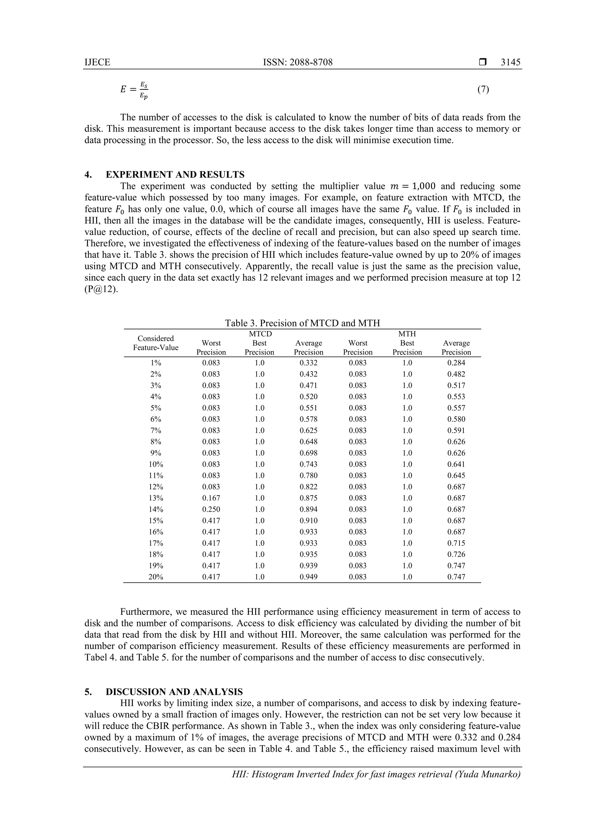
This document summarizes a research paper that proposes a new indexing structure called Histogram Inverted Index (HII) to improve the speed of image retrieval in a content-based image retrieval (CBIR) system. HII is based on an inverted index structure commonly used in text retrieval, but modifies it to index histogram data generated from images using multi-texton histogram and co-occurrence descriptor features. The HII consists of a feature-value list, inverted list, and map. It normalizes feature values, considers image pairs for each feature-value, and limits candidate images to improve efficiency while maintaining accuracy. Boolean retrieval using HII extracts candidate images from the inverted list for a given query image.

1. International Journal of Electrical and Computer Engineering (IJECE)
Vol.8, No.5, October 2018, pp. 3140~3148
ISSN: 2088-8708, DOI: 10.11591/ijece.v8i5.pp3140-3148  3140
Journal homepage: http://iaescore.com/journals/index.php/IJECE
HII: Histogram Inverted Index for Fast Images Retrieval
Yuda Munarko, Agus Eko Minarno
Teknik Informatika, Universitas Muhammadiyah Malang, Indonesia
Article Info ABSTRACT
Article history:
Received Jul 22, 2017
Revised Feb 10, 2018
Accepted Mar 15, 2018
This work aims to improve the speed of search by creating an indexing
structure in Content Based Images Retrieval (CBIR) system. We utilised an
inverted index structure that usually used in text retrieval with a
modification. The modified inverted index is built based on histogram data
that generated using Multi Texton Histogram (MTH) and Multi Texton Co-
Occurrence Descriptor (MTCD) from 10,000 images of Corel dataset. When
building the inverted index, we normalised value of each feature into a real
number and considered pairs of feature and value that owned by a particular
number of images. Based on our investigation, on MTCD histogram of 5,000
data test, we found that by considering histogram variable values which
owned by maximum 12% of images, the number of comparison for each
query can be reduced by 67.47% in a rate, the precision is 82.2%, and the
rate of access to disk is 32.83%. Furthermore, we named our approach as
Histogram Inverted Index (HII).
Keyword:
CBIR
Histogram indexing
Inverted index
Copyright © 2018 Institute of Advanced Engineering and Science.
All rights reserved.
Corresponding Author:
Yuda Munarko,
Universitas Muhammadiyah Malang,
Jl. Raya Tlogomas 246, Malang, 65141, Indonesia.
Email: yuda@umm.ac.id
1. INTRODUCTION
The study of content based images retrieval (CBIR) can be traced back to the early of 1990. CBIR is
becoming popular and importance since there were limitations of the existing image retrieval system which
based on additional text annotation [1]. The limitations usually were related to the annotation process of large
images collection, since it was time-consuming; and the annotation validation, since it was highly subjective.
Another limitation was the lack of images semantic meaning, which was the main problem of the old system,
but it can be overcome by CBIR. By incorporating image features, the retrieved images are more likely
similar to the query in term of images content.
In general, most of CBIR researches were conducted to manipulate image features, started with the
extraction of features and then followed by the selection of useful features. The type of features can be
classified into low-level features and high-level features. The examples of low-level features extraction are
gray level co-occurrence matrix (GLCM) which extracts texture features [2], the extraction of texture and
HSV (Hue, Saturation, Value) color spatial features [3], the use of color descriptor for color extraction [4],
and low-level shape extraction [5]. In another side, high-level features usually incorporated feedback from
the user to identify a particular concept. Moreover, several studies tried to combine more than one type of
features in order to increase CBIR performance. The example of this approach is Color Difference Histogram
(CDH) which utilizes color, texture, and shape simultaneously [6] and the combination of the CDH and
GLCM for extracting features from batik images [7]. Furthermore, there was also approach called micro-
structure descriptor (MSD) [8] which was also used to extract features from batik images [9]. Consequently,
the combination feature types will produce more features from every image. To be more detail, there are 72
features of MSD, 102 features of CDH, 82 features of MTH, and 98 features of MTCD. A large number of
features, when combined with a large number of images, causes CBIR suffer for a slow query process.

2. IJECE ISSN: 2088-8708 
HII: Histogram Inverted Index for fast images retrieval (Yuda Munarko)
3141
In order to increase query speed, CBIR should implement indexing techniques, so the images data
can be stored and retrieved effectively. A study by Je‘gou showed the use of nearest neighbor search with the
size of the index was between hundreds and millions which is similar to hash index concept [10]. This
approach, then, extends by [11] by implementing multi index concept. Conceptually, [10] and [11] also
implemented the inverted index which was usually utilized in text retrieval system. The use of inverted index
was also proposed by Squire et. al. along with relevance feedback [12]. Inverted file seemed to be able to
manage images data with more than 80,000 features, however, there is no further measurement for its
performance, and thus, the measurement was for the use of relevance feedback [12]. Moreover, the inverted
index was successfully adapted by other state of the art studies, such as, the use of two dimensional inverted
index which combines SIFT and color features, and additional co-indexing which based on semantic
features [13], and multi level index fusion by combining several features into groups and then organized each
group into different level [14].
Grouping features which called product quantization is an effective method to limit the size of
features and contribute to storage and memory use reduction. This approach was demonstrated by [10], [11],
and [14]. However, the implementation of this approach should be conducted carefully because wrong
features combination may reduce accuracy. Therefore, it is necessary to implement different quantization,
local quantization, which conserve the information of each feature but may limit memory and storage use for
indexing.
Thus, this study was conducted to investigate the implementation of an inverted index for CBIR,
including feature-value list, inverted list, map, and local quantization approach. We have proposed a strategy
to reduce space for indexing, to limit access to the disk, and to limit the number of candidate images so CBIR
has better efficiency and effectiveness. Features that indexed are those that generated using MTH [15] and
MTCD [16].
2. INVERTED INDEX
The CBIR indexing system that proposed is based on an inverted index which firstly implemented
by Frakes and Baeza-Yates [17] for the text based document. In that implementation, the inverted index was
built to make boolean retrieval process run faster. The result of boolean retrieval was a list of candidate
documents which may similar to the query. Moreover, the candidate documents were presented in order,
based on the similarity value. In general, the inverted index is useful in term of limiting the number of
candidate document that may similar to the query. As the result, the system does not need to compare the
query to all documents in the collection.
The implementation of the inverted index for text based document retrieval is shown in Figure 1.
There are three main components, a key list, an inverted list, and a map. The key list is a pair of a key and a
pointer, which the key usually is a term in a documents collection and the pointer is an integer value that
records the position of all documents that contains the key in an inverted list. Furthermore, for each key,
there is a list of documents which stored in an inverted list and there is only one inverted list that required for
storing lists of documents for all keys. Moreover, the map is a mapping of an id of a document to its physical
object.
Figure 1. The structure of inverted index

3.  ISSN: 2088-8708
IJECE Vol. 8, No. 5, October 2018 : 3140 – 3148
3142
The key list and the inverted list are developed by parsing all documents in the collection in order to
determine pairs of term and document id, and then store these pairs into a map structure. After parsing each
document, the data in the map structure are saved in a key list and an inverted list. Along with term and
document id, in the key list and the inverted list, there is information about the number of appearance of a
term in a particular document, named term frequency (tf), and the number of documents that contain the
term, named document frequency (df). The physical implementation of this list is shown in Figure 1., while
the inverted index usually has a structure like below:
< document_frequency, document_id, term_frequency, document_id, term_frequency, ..., ... >
Lastly, the map is a list of pairs of document id and the correspondent document. The correspondent
document can be a path of the document, a web link, or the document itself.
In the CBIR system, we modified the key so it will maintain images’ feature that contains number
rather than a term. This modification, then, is described in sub section 3.2.
3. RESEARCH METHOD
3.1. The Dataset
The datasets used are 10,000 images of Corel dataset and 5,000 images of Corel dataset. The first
dataset is used to develop index and searching object, and the second dataset is used as image query. Images
inside these datasets are then extracted using MTCD and MTH, so there are 98 features of MTCD and 82
features of MTH. An example of extraction result is presented in Table 1.
Table 1. The Example of Features Extraction Result
MTCD Feature1,2,3,4,5,6,... ,97,98
Img 1 0.0, 0.0, 0.0, 0.0, 45.5, 212.666666666667, ... , 0.662995696059771, 0.505170791008612
Img 2 0.0, 0.0, 0.0, 0.0, 43.0, 175.0, ... , 0.50380652272022, 0.339278153525531
MTH Feature1,2,3,4,5,6,... ,81,82
Img 1 0.0, 0.0, 0.0, 0.0, 48.25, 212.75, ... , 68.75, 138.25
Img 2 0.0, 0.0, 0.0, 0.0, 46.0, 173.5, ... , 58.0, 111.25
Most feature values are decimal, so it is not efficiently stored in the index. The reason is the index
size will be very large and it is possible that the feature value is too specific for a single image. So the feature
value needs to be normalised to a real number using (1). The equation, local quantization, works by
multiplying feature value 𝐹𝑣 by a real number 𝑚 and then rounded up or down depending on which one is
nearest. 𝑚 is empirically determined multiplier, customised based on the feature extraction algorithm used
and the results.
𝐹𝑣
′
= 𝑟𝑜𝑢𝑛𝑑(𝑚. 𝐹𝑣) (1)
Examples of normalised values are shown in Table 2., using 𝑚 = 1,000 and the origin data from Table 1.
The value of 𝑚 has a contribution to the range of normalised value, higher value causes wider range, in the
opposite, smaller value causes narrower range. A larger range has benefit for faster CBIR system
performance since the number of images candidate become smaller, however, it needs larger indexing
storage. Moreover, there is also an indication that very high multiplier value tend to cause overfitting, so it
possibly decreases recall value.
Table 2. The Example of Features Normalisation
MTCD Feature1,2,3,4,5,6,... ,97,98
Img 1 0, 0, 0, 0, 45500, 212667, ... , 663, 505
Img 2 0, 0, 0, 0, 43000, 175000, ... , 504, 339
MTH Feature1,2,3,4,5,6,... ,81,82
Img 1 0, 0, 0, 0, 48250, 212750, ... , 68750, 138250
Img 2 0, 0, 0, 0, 46000, 173500, ... , 58000, 111250
3.2. Histogram inverted index (HII)
In this paper, we propose indexing system for CBIR by modifying inverted index concept, which
named Histogram Inverted Index (HII). Components used in this approach are similar to the traditional

4. IJECE ISSN: 2088-8708 
HII: Histogram Inverted Index for fast images retrieval (Yuda Munarko)
3143
inverted index, those are a key list, which called feature-value list, an inverted list, and a map. The structure
of HII is presented in Figure 2.
The feature-value list is a list that contains feature-values, which each feature-value is composed of
a combination of feature number Fx and its value. For illustration, if there are 82 image features and each
feature has 100 different values, hence the size of the feature-value list is 8,200 feature-value. However, the
number of different values in each feature may vary, therefore, in databases or files, feature-values are stored
ascending by the number of feature and its value along with information about the number of values for each
feature. To figure out, let see Figure 3. where #𝑉𝑥 is the number of different values of feature 𝐹𝑥, and
𝑝𝑜𝑖𝑛𝑡𝑒𝑟𝑥_𝑦 is a pointer to a position in an inverted list that contains corresponding images.
Figure 2. The structure of histogram inverted index
Figure 3. The implementation of Feature-value list into file
Furthermore, the inverted list in HII is similar to the inverted list in text based information retrieval,
containing image-id for each feature-value in the feature-value list. Figure 2. shows the implementation of
the inverted list, for example, feature 𝐹1 with 𝑉1_2 value has < 𝑖𝑑25, 𝑖𝑑50, 𝑖𝑑101, . . . > images, and feature 𝐹2
with 𝑉2_1 value has < 𝑖𝑑35, 𝑖𝑑50, 𝑖𝑑200, . . . > images. Since there is a different number of images for each key,
so the information of images count #𝑉𝑥_𝑦 should be also stored, as shown in Figure 4.

5.  ISSN: 2088-8708
IJECE Vol. 8, No. 5, October 2018 : 3140 – 3148
3144
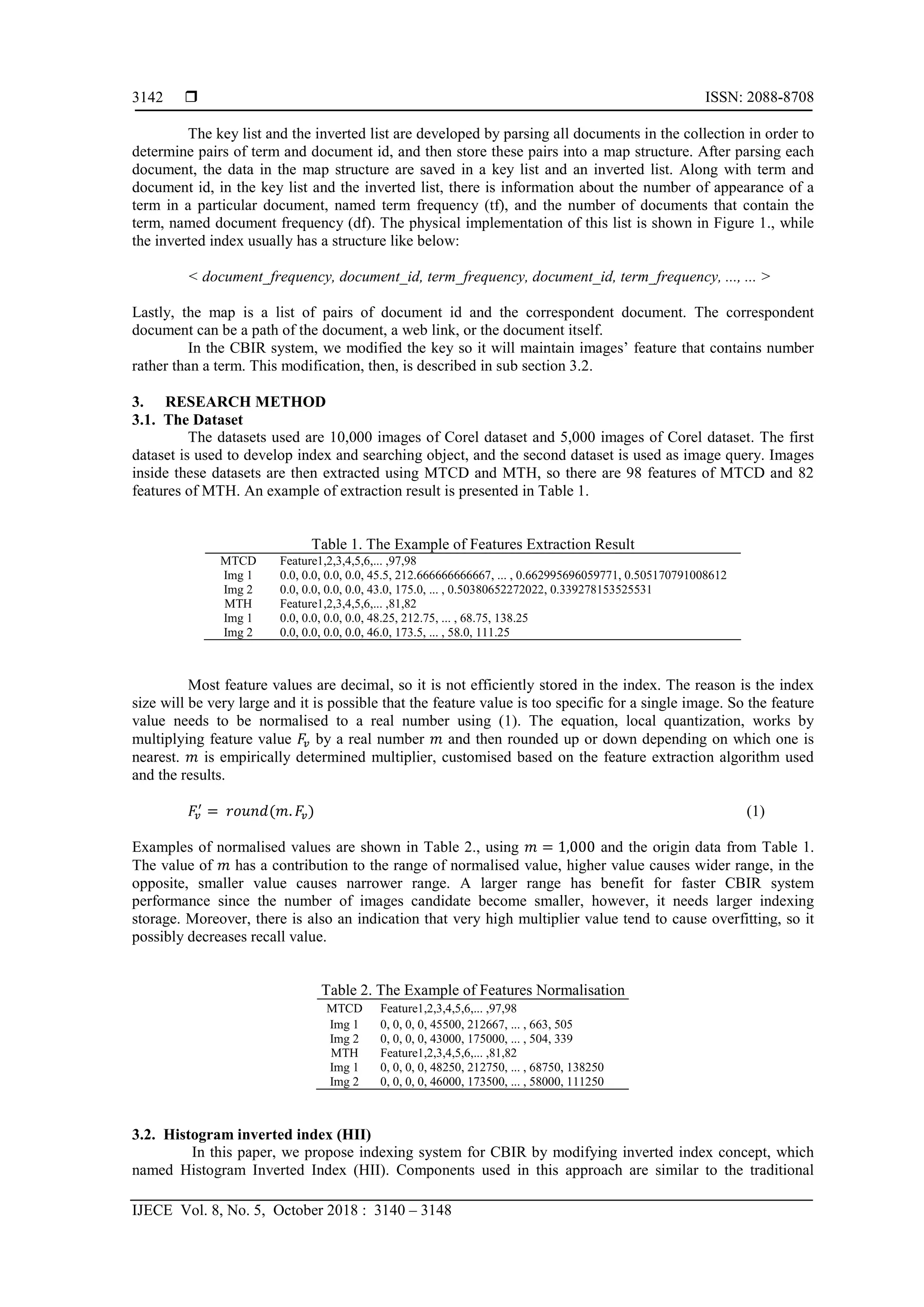
Figure 4. The implementation of inverted list into file
Lastly, the map which is also similar to the map of the standard inverted index. This map contains a
pair of image-id and name of file or image path.
3.3. Boolean retrieval
By utilising HII, it is possible to retrieve candidate images by performing boolean retrieval process
through image collection. The boolean retrieval process begins by extracting the features in the query image
using a suitable algorithm, so there are feature-value pairs as many as the number of features. Using these
feature-values, all images that have at least one the same key can be extracted from an inverted list. After
that, the candidate images are selected from the extracted images by operating boolean retrieval with OR,
AND, or both operators to the query image. In this paper, we used OR boolean operator, so all extracted
images automatically became candidate images. Finally, distance measurement is calculated between the
query image and the candidate images and then presenting the candidate images in sequence order from the
smallest to the largest distance.
3.4. Distance measurement
Distance measurement that used was Modified Canberra Distance [6] as shown in (2), where
𝑇 = [𝑇1, 𝑇2, . . . , 𝑇 𝑚] is an image in a data train with m features, and 𝑄 = [𝑄1, 𝑄2, . . . , 𝑄 𝑚] is an image in data
test with m features. Whereas 𝜇𝑇 and 𝜇𝑄 are the average value of all features for the data train images and
the data test images respectively.
𝐷(𝑇, 𝑄) = �
|𝑇 𝑖−𝑄 𝑖|
|𝑇 𝑖+𝜇𝑇|+|𝑄 𝑖+𝜇𝑄|
𝑚
𝑖=1
(2)
𝜇𝑇 = ∑
𝑇 𝑖
𝑚
𝑚
𝑖=1 (3)
𝜇𝑄 = ∑
𝑄 𝑖
𝑚
𝑚
𝑖=1 (4)
This measurement was used as a standard measurement in MTCD [15]. With this method, there is a
guarantee that all features will have the same effect on the distance measure calculation. For example, if there
is a feature 𝐹1 with a range of values from 1,000 to 10,000 and there is a feature 𝐹2 with a range of values
from 1 to 100 then 𝐹1 will not dominate the overall calculation.
3.5. Performance evaluation
System performance is tested using precision, recall, the proportion of execution, and the amount of
access to the disk. Precision is a comparison between the correct retrieval result 𝐼𝑐 and the total retrieval
result 𝐼𝑟, shown in the (5). While the recall is a comparison between the correct retrieval results 𝐼𝑐 and the
total number of relevant images in the database 𝐼 𝑑𝑏, indicated by the Equation 6.
𝑃𝑟𝑒𝑐𝑖𝑠𝑖𝑜𝑛 =
𝐼 𝑐
𝐼 𝑟
(5)
𝑅𝑒𝑐𝑎𝑙𝑙 =
𝐼 𝑐
𝐼 𝑑𝑏
(6)
Whereas the proportion of execution and the amount of access to disk are presented as efficiency
measure 𝐸 which is a comparison between the performance of proposed system compared to the performance
of base system, indicated by (7).

6. IJECE ISSN: 2088-8708 
HII: Histogram Inverted Index for fast images retrieval (Yuda Munarko)
3145
𝐸 =
𝐸 𝑠
𝐸 𝑝
(7)
The number of accesses to the disk is calculated to know the number of bits of data reads from the
disk. This measurement is important because access to the disk takes longer time than access to memory or
data processing in the processor. So, the less access to the disk will minimise execution time.
4. EXPERIMENT AND RESULTS
The experiment was conducted by setting the multiplier value 𝑚 = 1,000 and reducing some
feature-value which possessed by too many images. For example, on feature extraction with MTCD, the
feature 𝐹0 has only one value, 0.0, which of course all images have the same 𝐹0 value. If 𝐹0 is included in
HII, then all the images in the database will be the candidate images, consequently, HII is useless. Feature-
value reduction, of course, effects of the decline of recall and precision, but can also speed up search time.
Therefore, we investigated the effectiveness of indexing of the feature-values based on the number of images
that have it. Table 3. shows the precision of HII which includes feature-value owned by up to 20% of images
using MTCD and MTH consecutively. Apparently, the recall value is just the same as the precision value,
since each query in the data set exactly has 12 relevant images and we performed precision measure at top 12
(P@12).
Table 3. Precision of MTCD and MTH
Considered
Feature-Value
MTCD MTH
Worst
Precision
Best
Precision
Average
Precision
Worst
Precision
Best
Precision
Average
Precision
1% 0.083 1.0 0.332 0.083 1.0 0.284
2% 0.083 1.0 0.432 0.083 1.0 0.482
3% 0.083 1.0 0.471 0.083 1.0 0.517
4% 0.083 1.0 0.520 0.083 1.0 0.553
5% 0.083 1.0 0.551 0.083 1.0 0.557
6% 0.083 1.0 0.578 0.083 1.0 0.580
7% 0.083 1.0 0.625 0.083 1.0 0.591
8% 0.083 1.0 0.648 0.083 1.0 0.626
9% 0.083 1.0 0.698 0.083 1.0 0.626
10% 0.083 1.0 0.743 0.083 1.0 0.641
11% 0.083 1.0 0.780 0.083 1.0 0.645
12% 0.083 1.0 0.822 0.083 1.0 0.687
13% 0.167 1.0 0.875 0.083 1.0 0.687
14% 0.250 1.0 0.894 0.083 1.0 0.687
15% 0.417 1.0 0.910 0.083 1.0 0.687
16% 0.417 1.0 0.933 0.083 1.0 0.687
17% 0.417 1.0 0.933 0.083 1.0 0.715
18% 0.417 1.0 0.935 0.083 1.0 0.726
19% 0.417 1.0 0.939 0.083 1.0 0.747
20% 0.417 1.0 0.949 0.083 1.0 0.747
Furthermore, we measured the HII performance using efficiency measurement in term of access to
disk and the number of comparisons. Access to disk efficiency was calculated by dividing the number of bit
data that read from the disk by HII and without HII. Moreover, the same calculation was performed for the
number of comparison efficiency measurement. Results of these efficiency measurements are performed in
Tabel 4. and Table 5. for the number of comparisons and the number of access to disc consecutively.
5. DISCUSSION AND ANALYSIS
HII works by limiting index size, a number of comparisons, and access to disk by indexing feature-
values owned by a small fraction of images only. However, the restriction can not be set very low because it
will reduce the CBIR performance. As shown in Table 3., when the index was only considering feature-value
owned by a maximum of 1% of images, the average precisions of MTCD and MTH were 0.332 and 0.284
consecutively. However, as can be seen in Table 4. and Table 5., the efficiency raised maximum level with

7.  ISSN: 2088-8708
IJECE Vol. 8, No. 5, October 2018 : 3140 – 3148
3146
the average comparison reductions were 91.51% for MTCD and 93.29% for MTH, and the average access to
disc reductions were 91.46% for MTCD and 92.31% for MTH. Therefore, it can be said that maximum
efficiency leads to the decrease of retrieval effectivity.
Consequently, in order to get a better precision, the limit for maximum feature-value owned by
images should be increased. For example, when the limit was 10%, the average precisions were 0.743 for
MTCD and 0.641 for MTH. Furthermore, the precisions increased dramatically to 0.949 and 0.747 for
MTCD and MTH consecutively when the limit was 20%. Therefore, in general, there is a trade off between
efficiency and effectivity, it depend on the limit value and the type of feature extraction.
As an illustration, Figure 5. shows the increase of MTCD precision along with the decrease of
comparison efficiency and access to disk efficiency. If there is an assumption that CBIR system is rated as
effective when the precision is more than 80%, so the considered feature-value that owned by images should
be 12%. This setting will produce comparison efficiency 67.47% and access to disk efficiency 67.17%. To be
more detail, we can see that the comparison and access to disk efficiencies increase in almost a very similar
value linearly. Moreover, the decrease of precision along with the decrease of efficiencies is also linear.
Table 4. The Efficiency of Comparison of HII
Considered
Feature-Value
MTCD MTH
Worst
Precision
Best
Precision
Average
Precision
Worst
Precision
Best
Precision
Average
Precision
1% 84.45% 97.70% 91.51% 86.16% 98.29% 93.29%
2% 78.73% 97.65% 88.09% 75.60% 97.54% 84.18%
3% 75.87% 97.65% 87.08% 71.06% 97.25% 83.02%
4% 70.83% 97.65% 85.62% 66.15% 97.25% 81.98%
5% 59.75% 97.65% 84.49% 66.15% 97.25% 81.85%
6% 58.55% 97.65% 83.68% 66.15% 97.25% 81.35%
7% 55.03% 97.65% 81.99% 66.15% 97.25% 81.09%
8% 51.67% 97.65% 80.59% 64.05% 97.25% 80.29%
9% 47.78% 97.08% 77.57% 64.05% 97.25% 79.46%
10% 43.74% 97.08% 74.28% 59.55% 97.25% 79.46%
11% 38.99% 95.35% 71.05% 58.38% 97.25% 79.13%
12% 34.31% 95.35% 67.47% 53.35% 96.26% 77.15%
13% 28.45% 90.91% 62.05% 53.35% 96.26% 77.15%
14% 28.45% 90.91% 58.84% 53.35% 96.26% 77.15%
15% 24.90% 90.91% 55.83% 53.35% 96.26% 77.15%
16% 19.05% 82.80% 51.57% 53.35% 96.26% 77.15%
17% 19.05% 82.80% 51.57% 48.54% 96.26% 75.50%
18% 18.78% 82.80% 51.16% 46.09% 96.26% 74.47%
19% 16.86% 82.80% 49.98% 44.16% 96.26% 72.53%
20% 16.86% 82.09% 46.45% 44.16% 96.26% 72.53%
Table 5. The Efficiency of Access to Disk of HII
Considered
Feature-Value
MTCD MTH
Worst
Precision
Best
Precision
Average
Precision
Worst
Precision
Best
Precision
Average
Precision
1% 84.35% 97.69% 91.46% 84.15% 98.03% 92.31%
2% 78.60% 97.63% 88.01% 72.01% 97.17% 81.80%
3% 75.71% 97.63% 87.00% 66.80% 96.84% 80.53%
4% 70.62% 97.63% 85.53% 61.16% 96.84% 79.33%
5% 59.38% 97.63% 84.39% 61.16% 96.84% 79.18%
6% 58.16% 97.63% 83.56% 61.16% 96.84% 78.60%
7% 54.60% 97.63% 81.86% 61.16% 96.84% 78.31%
8% 51.17% 97.63% 80.44% 58.69% 96.84% 77.39%
9% 47.31% 97.06% 77.40% 58.69% 96.84% 77.39%
10% 43.22% 97.06% 74.06% 53.44% 95.71% 76.43%
11% 38.40% 95.32% 70.80% 52.03% 95.71% 76.04%
12% 33.60% 95.32% 67.17% 46.20% 95.71% 73.77%
13% 27.64% 90.83% 61.66% 46.20% 95.71% 73.77%
14% 27.64% 90.83% 58.40% 46.20% 95.71% 73.77%
15% 24.29% 90.83% 55.34% 46.20% 95.71% 73.77%
16% 18.11% 82.66% 51.01% 46.20% 95.71% 73.77%
17% 18.11% 82.66% 51.01% 40.65% 95.71% 71.88%
18% 17.75% 82.66% 50.59% 37.74% 95.71% 70.68%
19% 15.74% 82.66% 49.40% 35.59% 95.71% 68.45%
20% 15.74% 81.91% 45.80% 35.59% 95.71% 68.45%

8. IJECE ISSN: 2088-8708 
HII: Histogram Inverted Index for fast images retrieval (Yuda Munarko)
3147
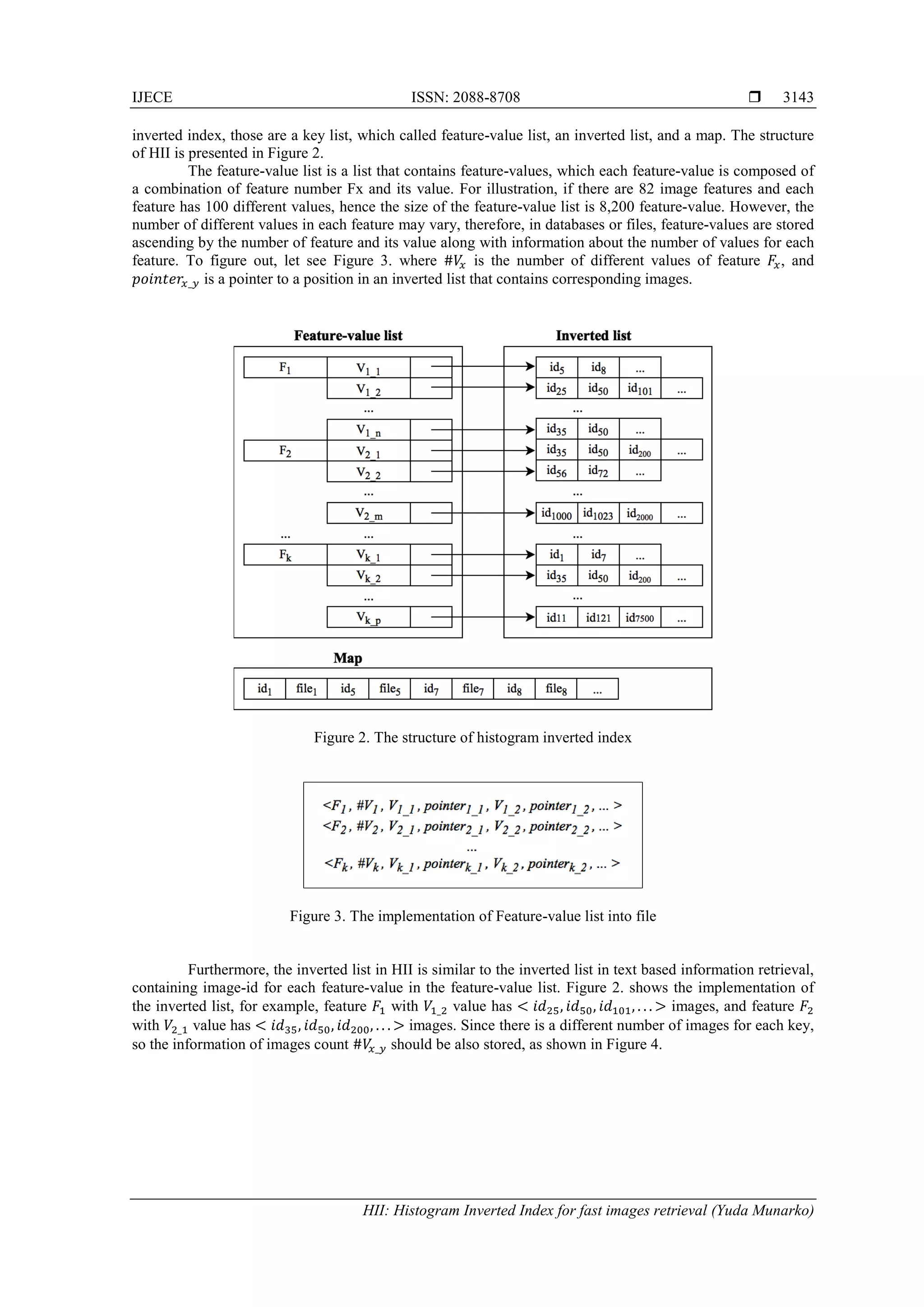
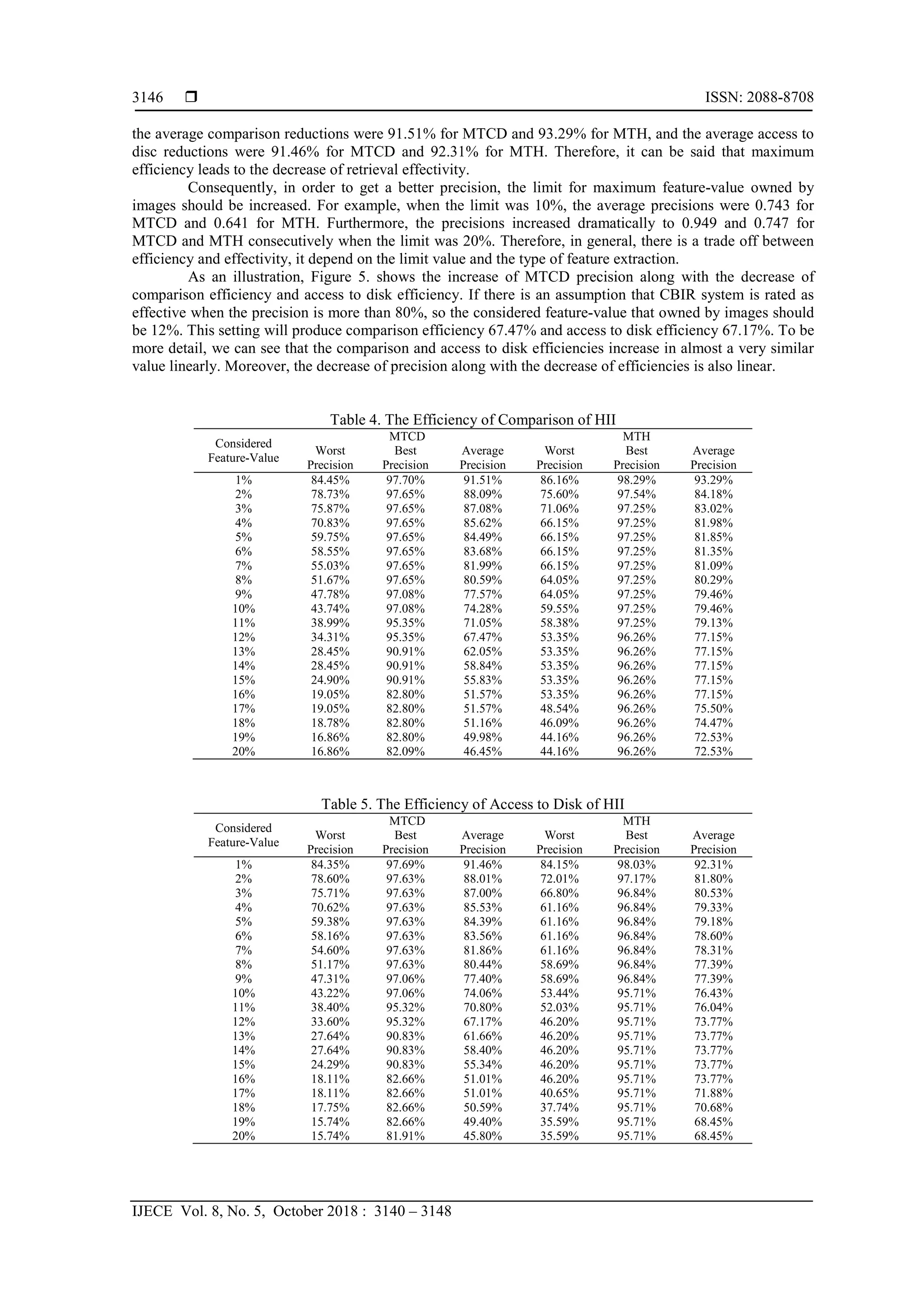
Figure 5. The HII performance for MTCD
6. CONCLUSION
Our work shows that the use of an inverted index for indexing image histograms that are generated
using MTH and MTCD is relatively effective and efficient. The approach is able to reduce the number of
comparison to only 32.53% for MTCD histogram and 27.46% for MTH histogram when considering feature-
value owned by 12% and 19% of MTCD and MTH respectively. By these reductions, the precision value for
each histogram is 0.822 for MTCD and 0.747 for MTH. We see that there are several attributes which have
the same value for the majority of images, so there is a possibility to prune those attributes. Therefore, the
next step of our work is investigating the pruning technique and the use of different multiplier value.
REFERENCES
[1] Y. Rui, T. S. Huang, and S.-F. Chang, “Image Retrieval: Current Techniques, Promising Directions, and Open
Issues,” Journal of visual communication and image representation, vol. 10, no. 1, pp. 39–62, 1999.
[2] R.M.Haralick,K.Shanmugametal.,“Textural Features for Image Classification,” IEEETransactionsonsystems, man,
and cybernetics, no. 6, pp. 610–621, 1973.
[3] Z. Lei, L. Fuzong, and Z. Bo, “A Cbir Method Based on Color-spatial Feature,” in TENCON 99. Proceedings of the
IEEE Region 10 Conference, vol. 1. IEEE, 1999, pp. 166–169.
[4] J.VanDeWeijerandC.Schmid, “Coloring Local Feature Extraction,”ComputerVision–ECCV2006,pp.334–348, 2006.
[5] S. Brandt, J. Laaksonen, and E. Oja, “Statistical Shape Features for Content-Based Image Retrieval,” Journal of
Mathematical Imaging and Vision, vol. 17, no. 2, pp. 187–198, 2002.
[6] G.-H.LiuandJ.-Y.Yang,“Content-based Image Retrieval using Color Differen Cehistogram,”PatternRecognition,
vol. 46, no. 1, pp. 188–198, 2013.
[7] A. E. Minarno and N. Suciati, “Batik Image Retrieval Based on Color Difference Histogram and Gray Level Co-
Occurrence Matrix,” TELKOMNIKA (Telecommunication Computing Electronics and Control), vol. 12, no. 3, pp.
597–604, 2014.
[8] G.-H. Liu, Z.-Y. Li, L. Zhang, and Y. Xu, “Image Retrieval Based on Micro-Structure Descriptor,” Pattern
Recognition, vol. 44, no. 9, pp. 2123–2133, 2011.
[9] A. E. Minarno, Y. Munarko, F. Bimantoro, A. Kurniawardhani, and N. Suciati, “Batik Image Retrieval Based on
Enhanced Micro-Structure Descriptor,” in Computer Aided System Engineering (APCASE), 2014 Asia-Pacific
Conference on. IEEE, 2014, pp. 65–70.
[10] H. Jegou, M. Douze, and C. Schmid, “Product Quantization for Nearest Neighbor Search,” IEEE transactions on
pattern analysis and machine intelligence, vol. 33, no. 1, pp. 117–128, 2011.
[11] A.BabenkoandV.Lempitsky,“The Inverted Multi-index,” inComputerVisionandPatternRecognition(CVPR), 2012
IEEE Conference on. IEEE, 2012, pp. 3069–3076.
[12] D. M. Squire, W. Mu ̈ller, H. Mu ̈ller, and T. Pun, “Content-based Query of Image Databases: Inspirations from
Text Retrieval,” Pattern Recognition Letters, vol. 21, no. 13, pp. 1193–1198, 2000.
[13] W. Lei and G. Xiao, “Image Retrieval using Two-dimensional Inverted Index and Semantic Attributes,”
in Software Engineering and Service Science (ICSESS), 2016 7th IEEE International Conference on. IEEE, 2016,
pp. 679–682.
[14] X. Chen, J. Wu, S. Sun, and Q. Tian, “Multi-index Fusion Via Similarity Matrix Pooling for Image Retrieval,”
in Communications (ICC), 2017 IEEE International Conference on. IEEE, 2017, pp. 1–6.

9.  ISSN: 2088-8708
IJECE Vol. 8, No. 5, October 2018 : 3140 – 3148
3148
[15] G.-H. Liu, L. Zhang, Y.-K. Hou, Z.-Y. Li, and J.-Y. Yang, “Image Retrieval Based on Multi-texton Histogram,”
Pattern Recognition, vol. 43, no. 7, pp. 2380–2389, 2010.
[16] A. E. MINARNO and N. SUCIATI, “Image Retrieval Using Multi Texton Co-Occurrence Descriptor.” Journal of
Theoretical & Applied Information Technology, vol. 67, no. 1, 2014.
[17] W. B. Frakes and R. Baeza-Yates, “Information Retrieval: Data Structures and Algorithms,” 1992.