Download as PDF, PPTX


![Introduction
1-24
ANSYS, Inc. Proprietary
© 2009 ANSYS, Inc. All rights reserved.
February 23, 2009
Inventory #002593
Training ManualTraining Manual
3-24
ANSYS, Inc. Proprietary
© 2009 ANSYS, Inc. All rights reserved.
February 20, 2009
Inventory #002704
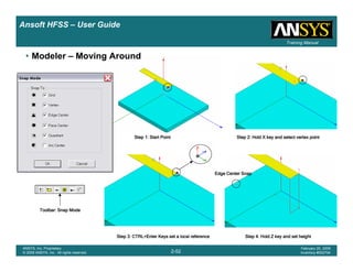
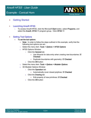
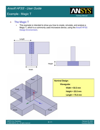
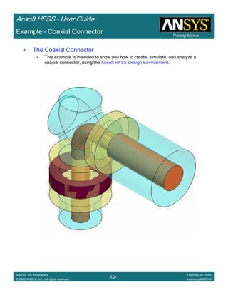
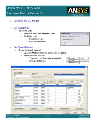
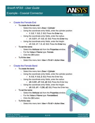
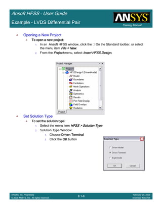
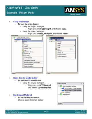
Ansoft HFSS – User Guide
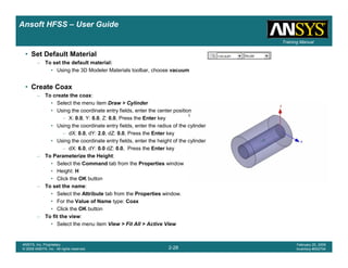
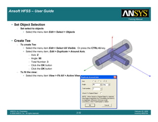
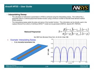
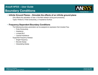
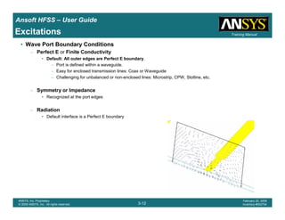
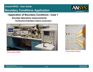
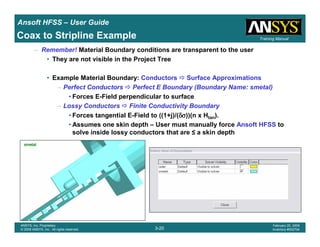
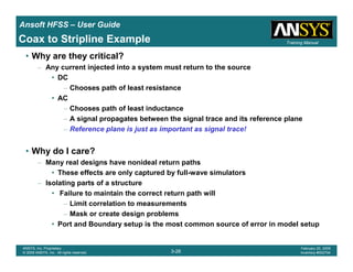
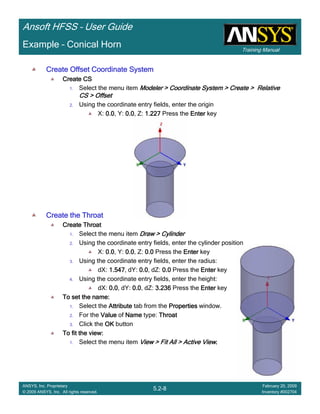
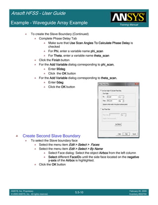
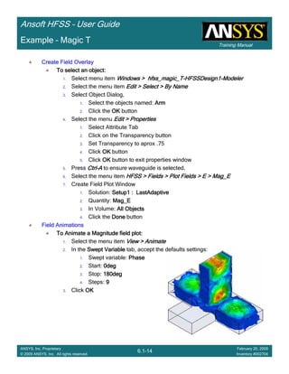
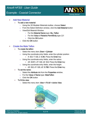
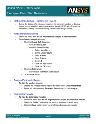
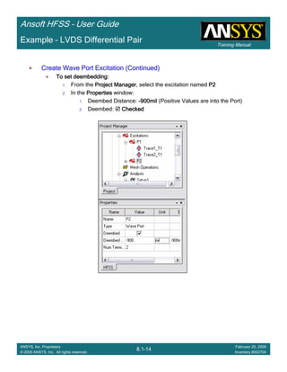
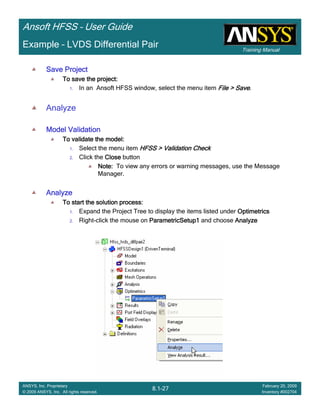
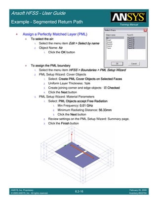
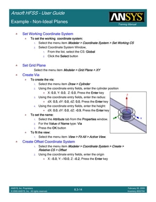
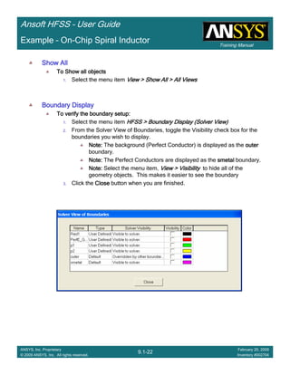
• How often is the Setup that Simple?
– If you are emulating laboratory measurements? [Case 1 ]
• Most of the time!
– Laboratory equipment does not directly connect to arbitrary transmission
lines
• Exceptions
– Emulating Complex Probes with a Port Understanding of Probe
– If you are isolating part of a structure? [Case 2 ]
• For “real” designs - usually only by dumb luck!
– User Must Understand and/or Implement Correctly:
1.Port Boundary conditions and impact of boundary condition
2.Fields within the structure
3.Assumptions made by port solver
4.Return path
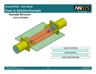
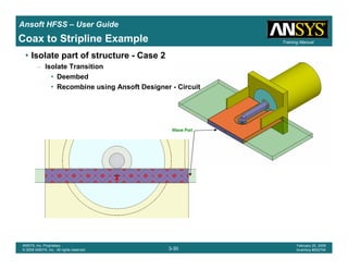
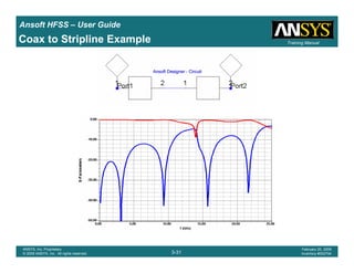
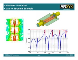
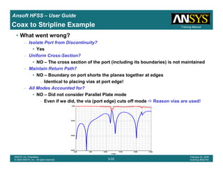
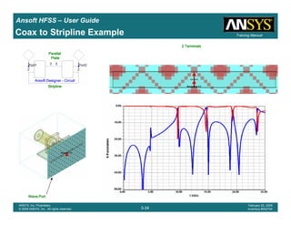
Coax to Stripline Example](https://image.slidesharecdn.com/hfssuser-guide-150114060507-conversion-gate02/85/Hfss-user-guide-120-320.jpg)
![Introduction
1-25
ANSYS, Inc. Proprietary
© 2009 ANSYS, Inc. All rights reserved.
February 23, 2009
Inventory #002593
Training ManualTraining Manual
3-25
ANSYS, Inc. Proprietary
© 2009 ANSYS, Inc. All rights reserved.
February 20, 2009
Inventory #002704
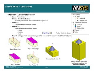
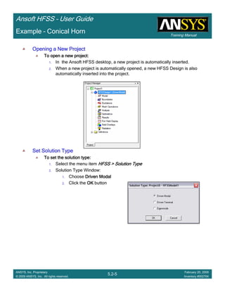
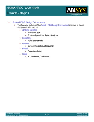
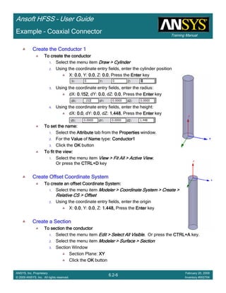
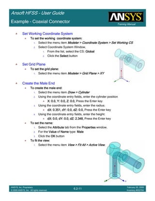
Ansoft HFSS – User Guide
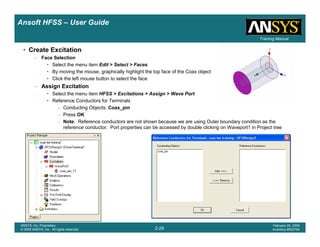
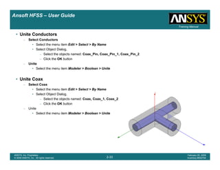
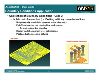
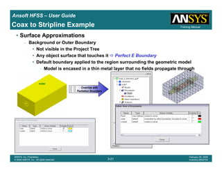
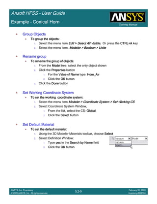
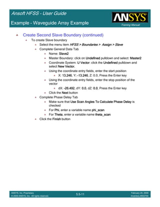
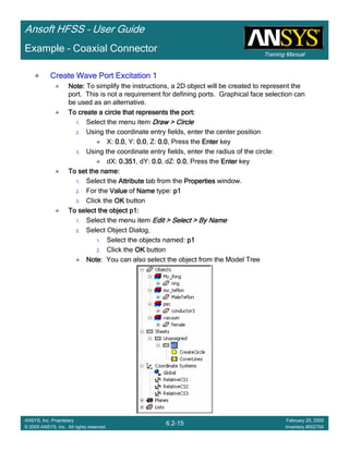
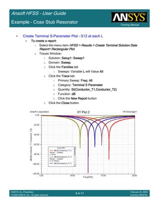
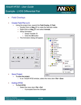
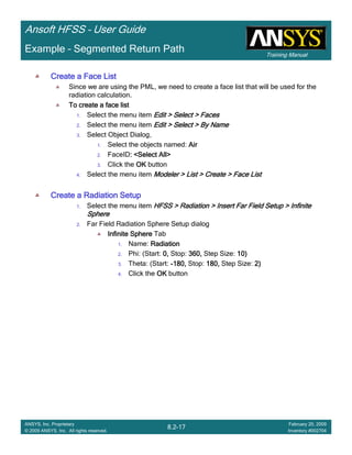
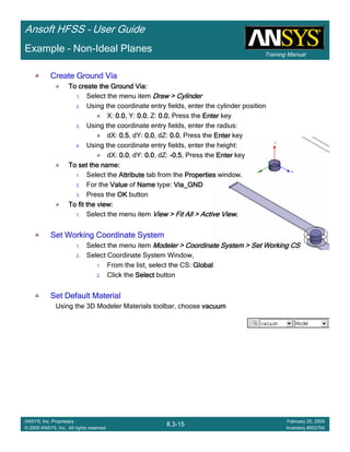
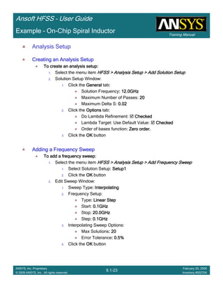
• Side Note: Problems Associated with Correlating Results [Case 2]
– Can be broken into two categories of problems
1.Complex Structure
– BGA, Backplane, Antenna Feed, Waveguide “Plumbing”, etc
– Most common problems result from
• Measurement setup – Test fixtures, deembedding, etc.
• Failing to understand the fields in the structure Boundary Problem
• Return path problems – Model truncation
2.Simple Structures
– Uniform transmission lines
• Equations or Circuit Elements
– Most common problems result from
• Improper use of default or excitation boundary conditions
• Failure to understand the assumptions used by “correct” results
(Equations or Circuit Elements)
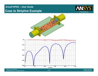
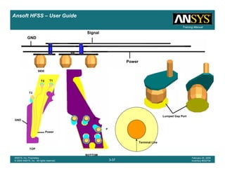
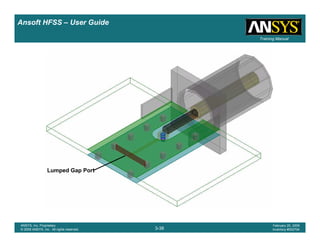
Coax to Stripline Example](https://image.slidesharecdn.com/hfssuser-guide-150114060507-conversion-gate02/85/Hfss-user-guide-121-320.jpg)


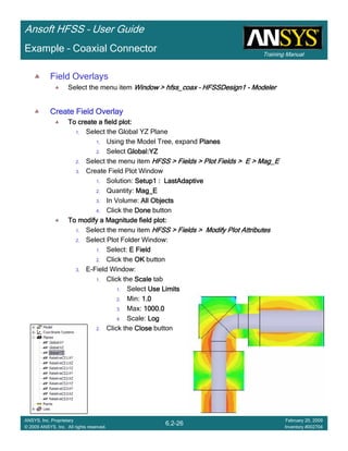
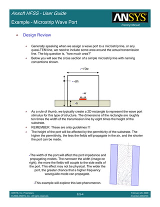
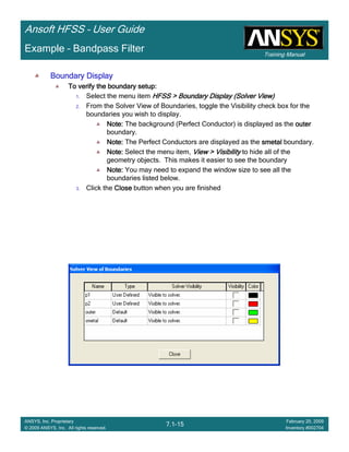
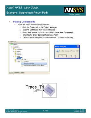
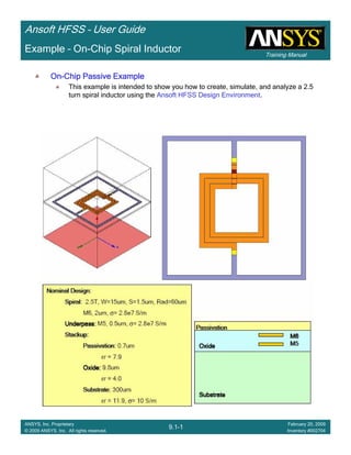
![Training Manual
Ansoft HFSS – User Guide
5.3-18
ANSYS, Inc. Proprietary
© 2009 ANSYS, Inc. All rights reserved.
February 20, 2009
Inventory #002704
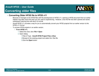
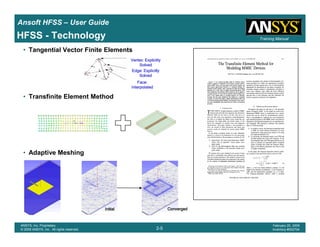
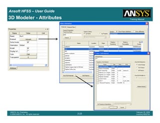
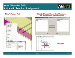
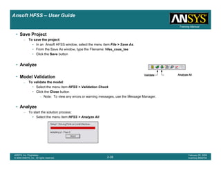
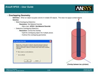
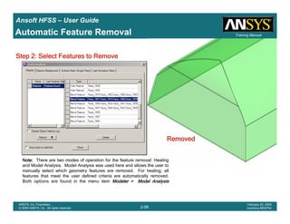
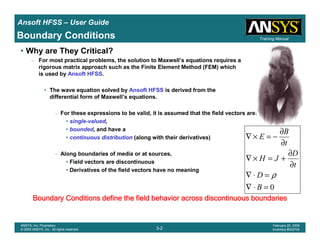
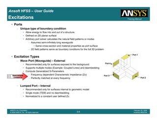
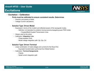
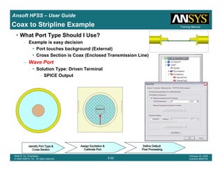
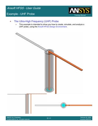
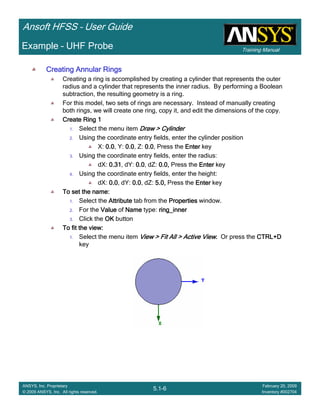
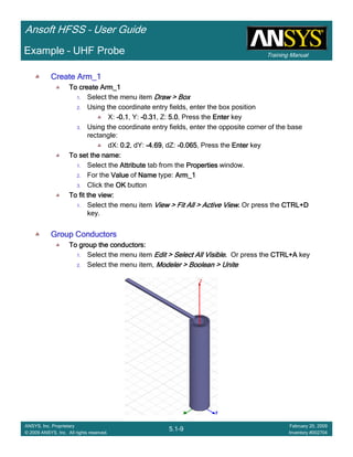
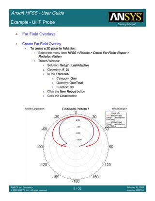
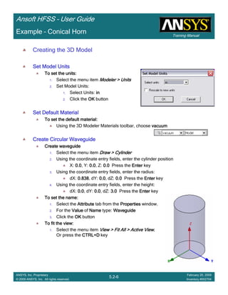
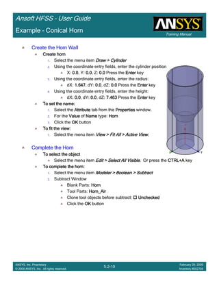
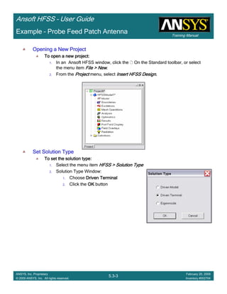
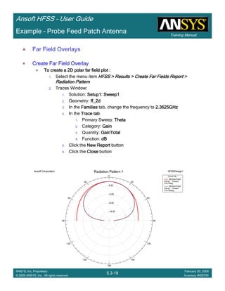
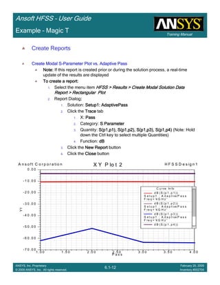
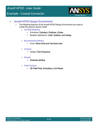
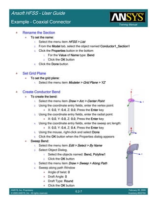
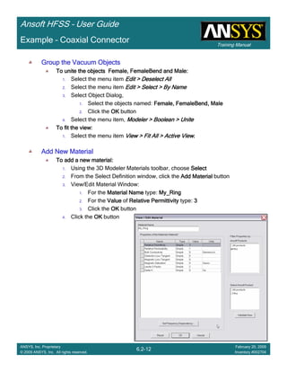
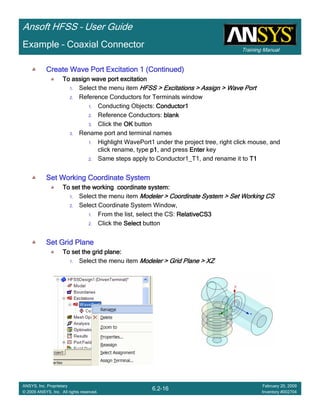
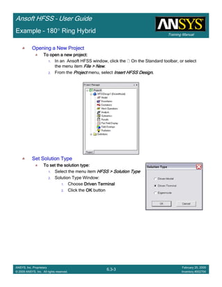
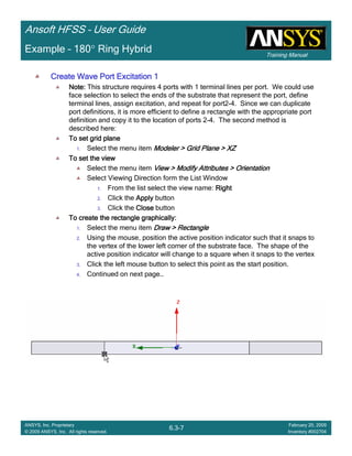
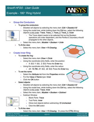
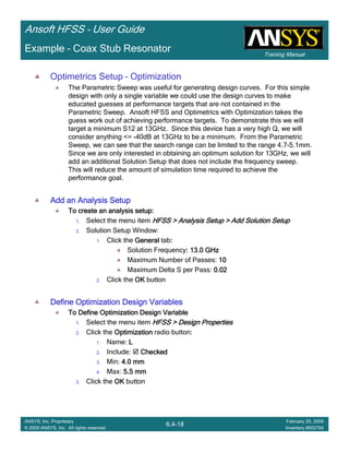
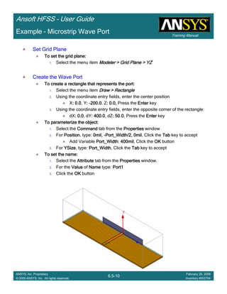
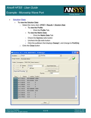
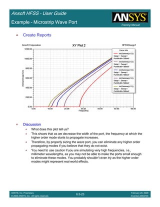
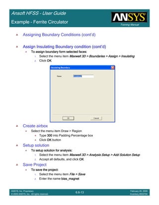
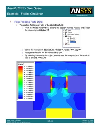
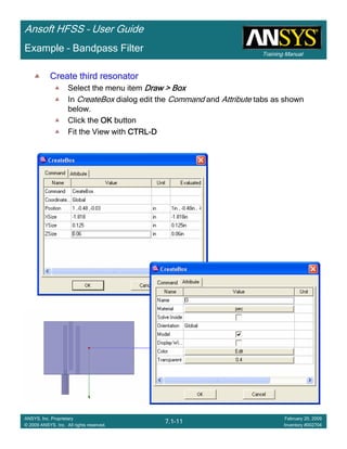
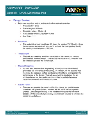
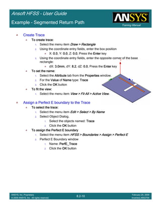
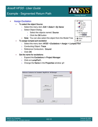
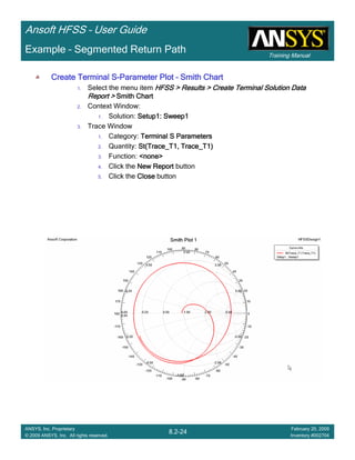
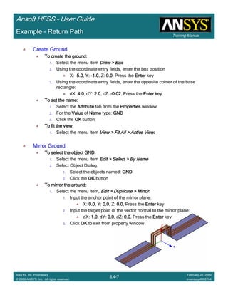
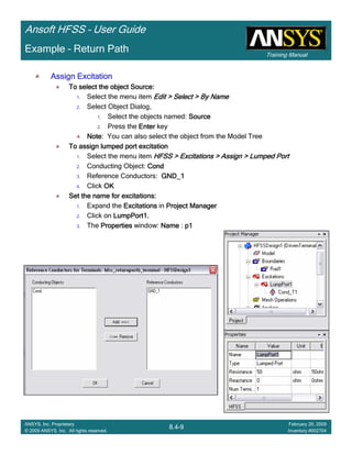
Example – Probe Feed Patch Antenna
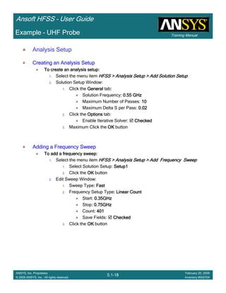
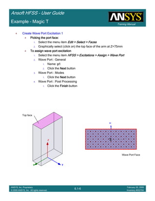
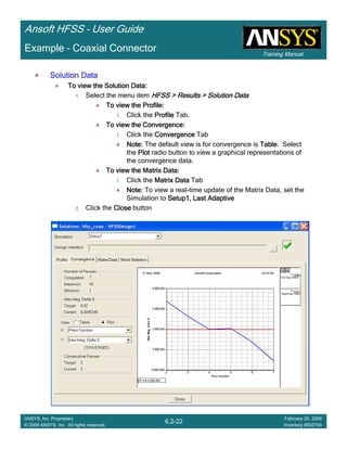
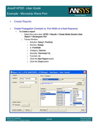
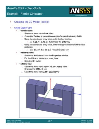
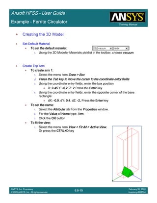
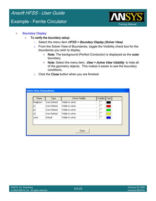
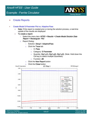
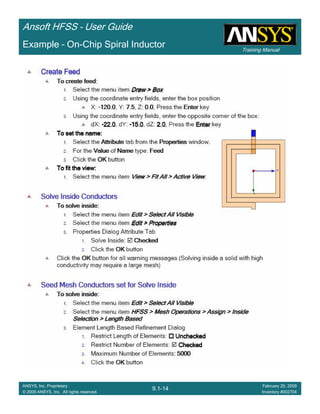
Create Reports
Create Terminal SCreate Terminal SCreate Terminal SCreate Terminal S----Parameter PlotParameter PlotParameter PlotParameter Plot ---- MagnitudeMagnitudeMagnitudeMagnitude
To create a report:To create a report:To create a report:To create a report:
1. Select the menu item HFSS > Results > Create Terminal Solution DataHFSS > Results > Create Terminal Solution DataHFSS > Results > Create Terminal Solution DataHFSS > Results > Create Terminal Solution Data
Report> Rectangular PlotReport> Rectangular PlotReport> Rectangular PlotReport> Rectangular Plot
2. Traces Window::::
1. Solution: Setup1: Sweep1Setup1: Sweep1Setup1: Sweep1Setup1: Sweep1
2. Domain: SweepSweepSweepSweep
3. Click the TraceTraceTraceTrace tab
1. Category: Terminal S ParameterTerminal S ParameterTerminal S ParameterTerminal S Parameter
2. Quantity: St(coax_pin_T1,coax_pin_T1)St(coax_pin_T1,coax_pin_T1)St(coax_pin_T1,coax_pin_T1)St(coax_pin_T1,coax_pin_T1) Function: dBdBdBdB
3. Click the New ReportNew ReportNew ReportNew Report button
4. Click the CloseCloseCloseClose button
Mark all tracesMark all tracesMark all tracesMark all traces
1. Select the menu item Edit > Select AllEdit > Select AllEdit > Select AllEdit > Select All
2. Select the menu item Report 2D > Marker > Add MinimumReport 2D > Marker > Add MinimumReport 2D > Marker > Add MinimumReport 2D > Marker > Add Minimum
3. When you are finished, select the menu item Report 2D > Marker > ClearReport 2D > Marker > ClearReport 2D > Marker > ClearReport 2D > Marker > Clear
AllAllAllAll to remove the marker.
1.00 1.50 2.00 2.50 3.00 3.50
Freq [GHz]
-25.00
-20.00
-15.00
-10.00
-5.00
0.00
dB(St(coax_pin_T1,coax_pin_T1))
Ansoft Corporation HFSSDesign1XY Plot 1
m1
Curve Info
dB(St(coax_pin_T1,coax_pin_T1))
Setup1 : Sweep1
Name X Y
m1 2.3625 -21.4575](https://image.slidesharecdn.com/hfssuser-guide-150114060507-conversion-gate02/85/Hfss-user-guide-226-320.jpg)


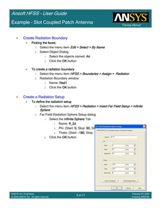
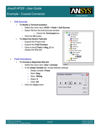
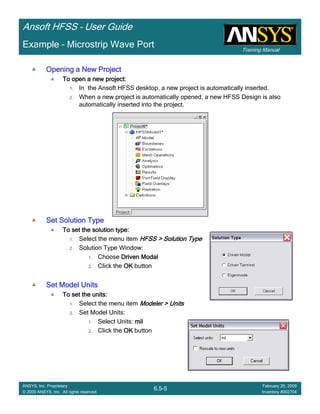
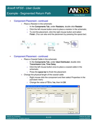
![Training Manual
Ansoft HFSS – User Guide
5.4-18
ANSYS, Inc. Proprietary
© 2009 ANSYS, Inc. All rights reserved.
February 20, 2009
Inventory #002704
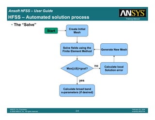
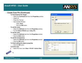
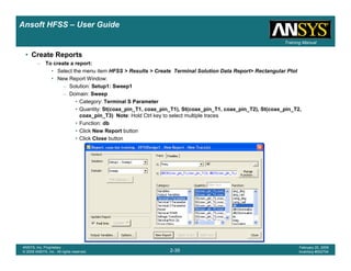
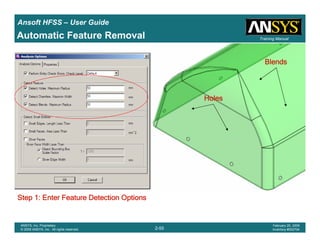
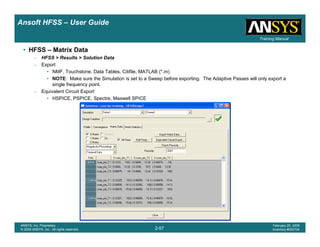
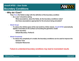
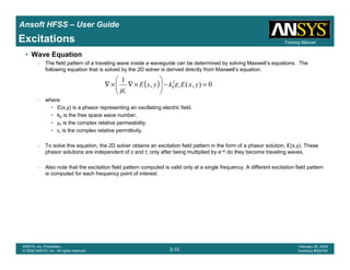
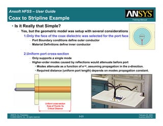
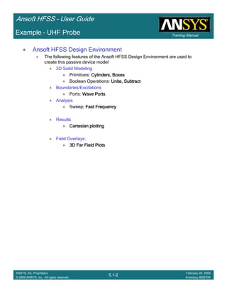
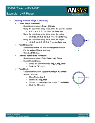
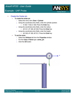
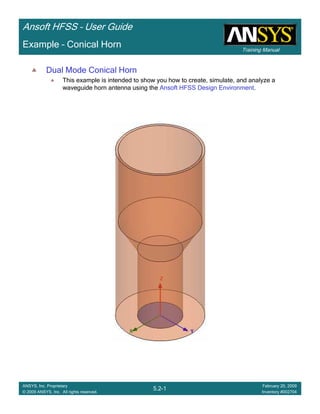
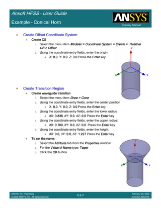
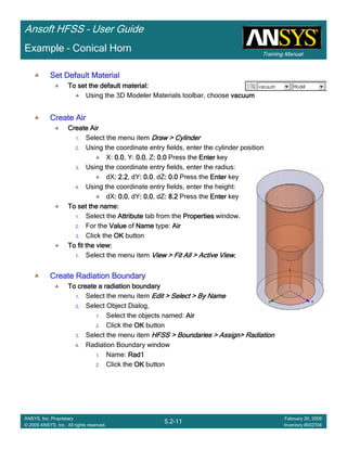
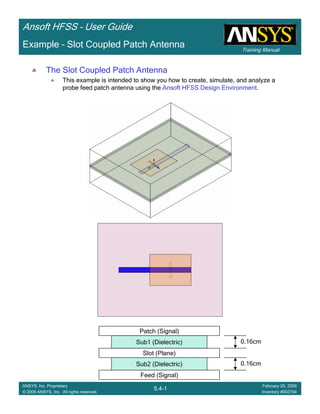
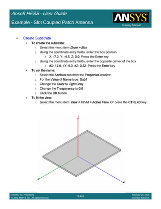
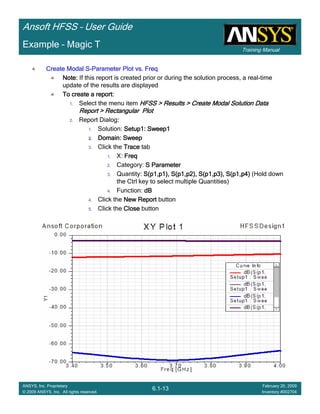
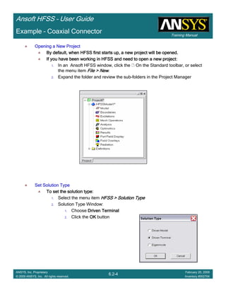
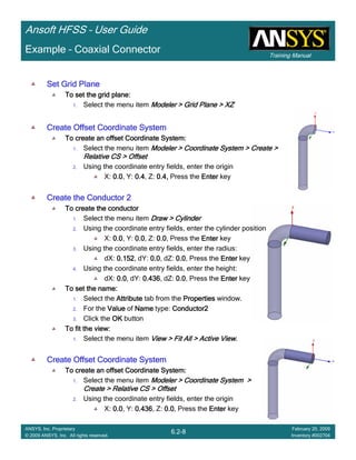
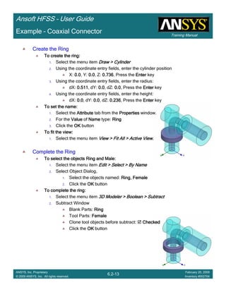
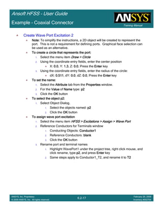
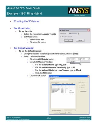
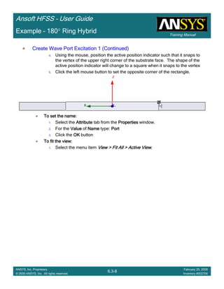
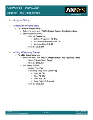
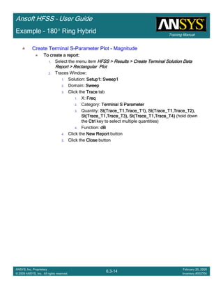
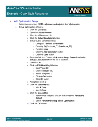
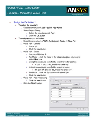
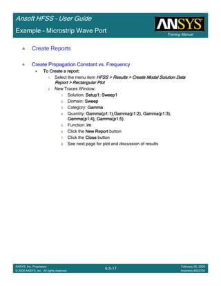
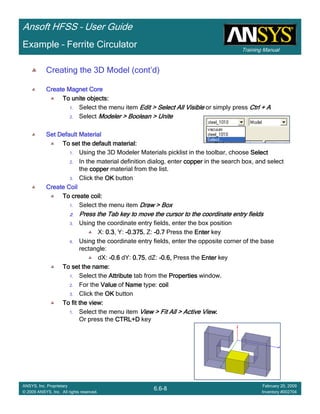
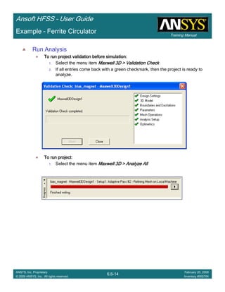
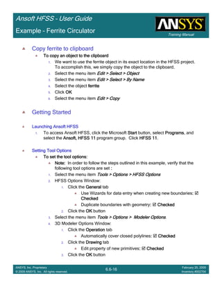
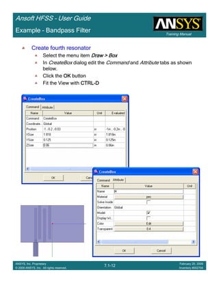
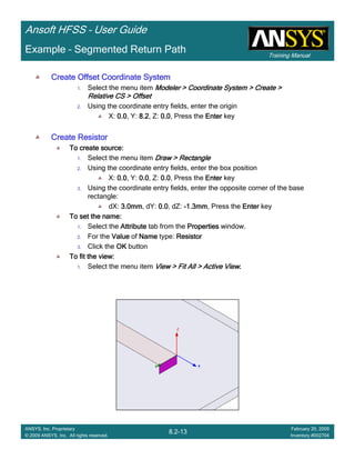
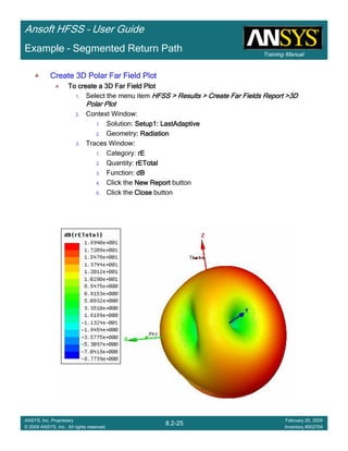
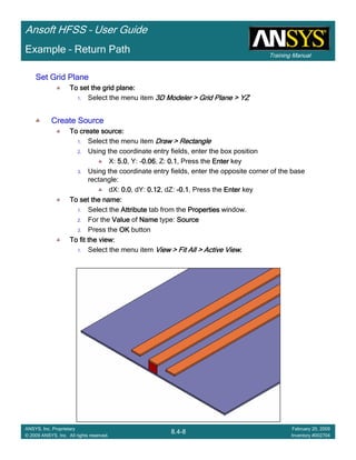
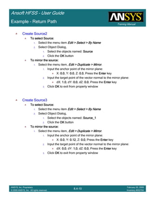
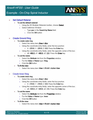
Example – Slot Coupled Patch Antenna
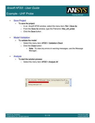
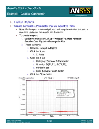
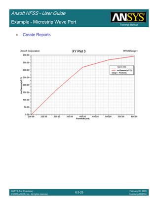
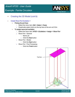
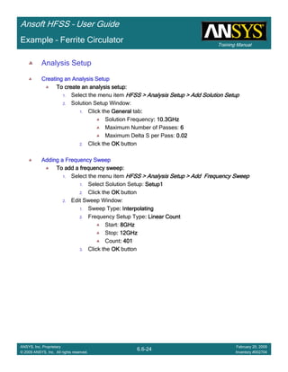
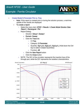
Create Reports
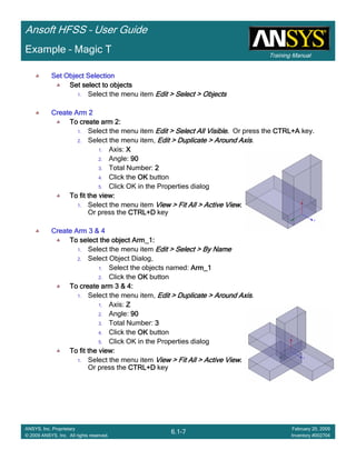
Create Terminal SCreate Terminal SCreate Terminal SCreate Terminal S----Parameter PlotParameter PlotParameter PlotParameter Plot ---- MagnitudeMagnitudeMagnitudeMagnitude
To create a report:To create a report:To create a report:To create a report:
1. Select the menu item HFSS > Results > Create Terminal Solution DataHFSS > Results > Create Terminal Solution DataHFSS > Results > Create Terminal Solution DataHFSS > Results > Create Terminal Solution Data
Report > Rectangular PlotReport > Rectangular PlotReport > Rectangular PlotReport > Rectangular Plot
2. Traces Window::::
1. Solution: Setup1: Sweep1Setup1: Sweep1Setup1: Sweep1Setup1: Sweep1
2. Domain: SweepSweepSweepSweep
3. Category: Terminal S ParameterTerminal S ParameterTerminal S ParameterTerminal S Parameter
4. Quantity: St(T1,T1),St(T1,T1),St(T1,T1),St(T1,T1),
5. Function: dBdBdBdB
6. Click the New ReportNew ReportNew ReportNew Report button
7. Click the CloseCloseCloseClose button
3. Add a minimum marker to the trace
1. Select the trace by left clicking on it
2. Go to Report2DReport2DReport2DReport2D >>>> MarkerMarkerMarkerMarker >>>> Add MinimumAdd MinimumAdd MinimumAdd Minimum
1.00 1.50 2.00 2.50 3.00 3.50
Freq [GHz]
-12.00
-10.00
-8.00
-6.00
-4.00
-2.00
0.00
dB(St(p1,p1))
Ansoft Corporation HFSSModel1XY Plot 1
m1
Curve Info
dB(St(p1,p1))
Setup1 : Sweep1
Name X Y
m1 2.2875 -10.1263](https://image.slidesharecdn.com/hfssuser-guide-150114060507-conversion-gate02/85/Hfss-user-guide-246-320.jpg)

![Training Manual
Ansoft HFSS – User Guide
5.5-1
ANSYS, Inc. Proprietary
© 2009 ANSYS, Inc. All rights reserved.
February 20, 2009
Inventory #002704
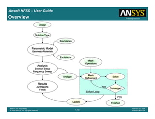
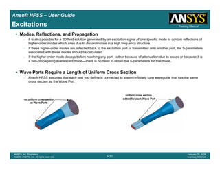
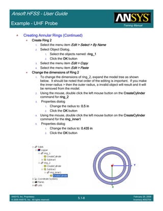
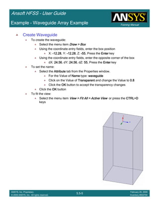
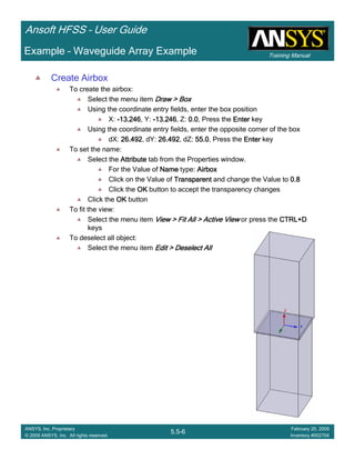
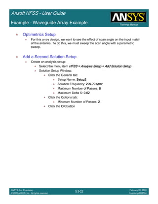
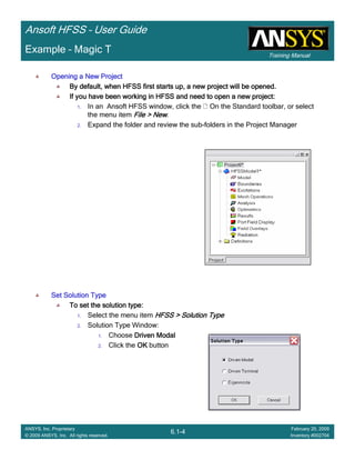
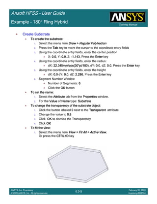
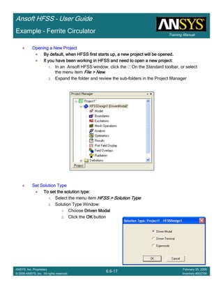
Example – Waveguide Array Example
The Waveguide Array
This example is intended to show you how to create, simulate, and analyze a
Waveguide array antenna using the Ansoft HFSS Design Environment
A WavePort will be used for the waveguide feed excitation
A Floquet Port will be used for the phased array’s free space excitation and
termination
Master/Slave boundary conditions will be used to create the array’s unit cell
Reference:
[1] N. Amitay, V. Galindo and C. Wu, “Theory and Analysis of Phased Array Antennas”, Wiley-Interscience,
1972, ISBN 0-471-02553-4, section5.2.1.](https://image.slidesharecdn.com/hfssuser-guide-150114060507-conversion-gate02/85/Hfss-user-guide-249-320.jpg)
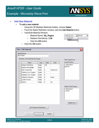
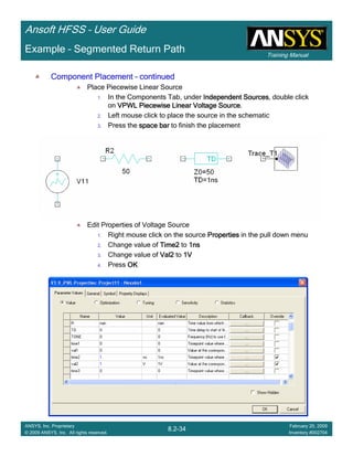
![Training Manual
Ansoft HFSS – User Guide
5.5-26
ANSYS, Inc. Proprietary
© 2009 ANSYS, Inc. All rights reserved.
February 20, 2009
Inventory #002704
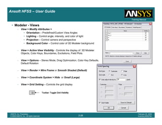
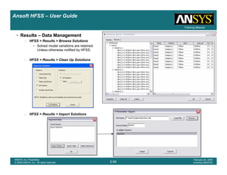
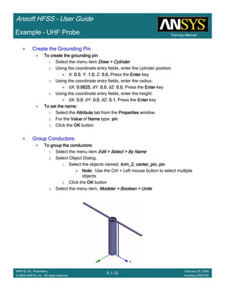
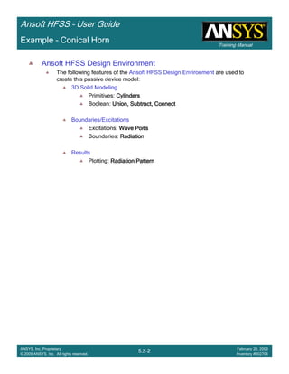
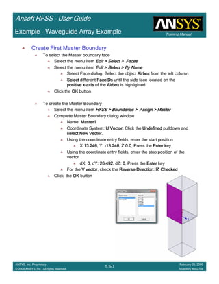
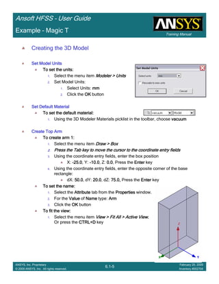
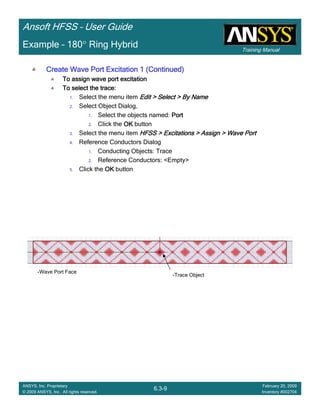
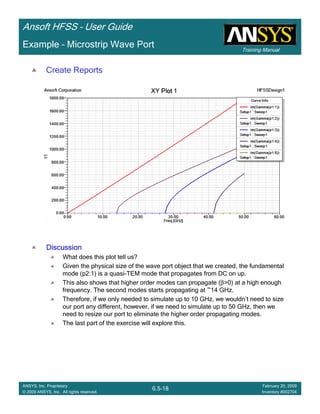
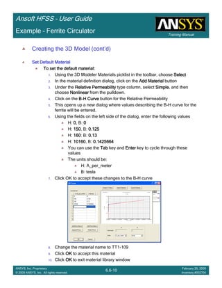
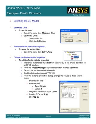
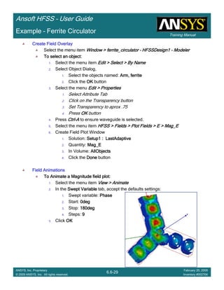
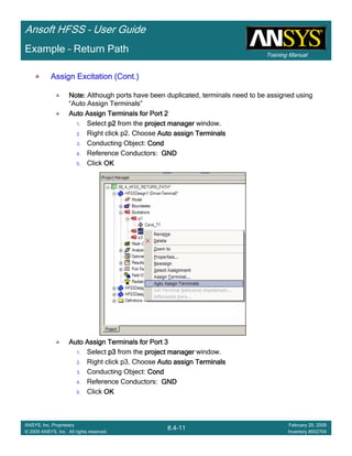
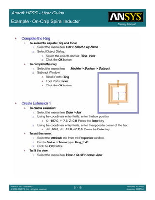
Example – Waveguide Array Example
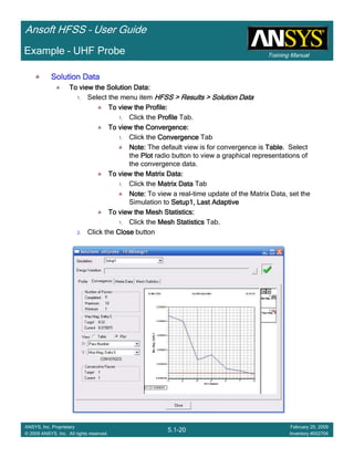
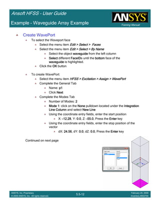
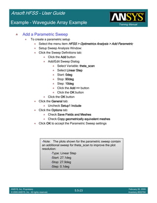
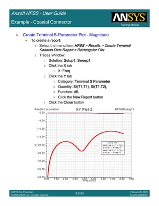
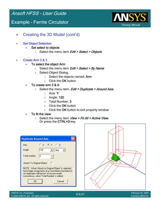
Create S-Parameter Plot
To create a report:
1. Select the menu item HFSS > Results > Create Modal Solution DataHFSS > Results > Create Modal Solution DataHFSS > Results > Create Modal Solution DataHFSS > Results > Create Modal Solution Data
Report > Rectangular PlotReport > Rectangular PlotReport > Rectangular PlotReport > Rectangular Plot
2. Traces Window::::
1. Solution: Setup2: LastAdaptiveSetup2: LastAdaptiveSetup2: LastAdaptiveSetup2: LastAdaptive
2. X: Switch to theta_scantheta_scantheta_scantheta_scan
3. Category: S ParameterS ParameterS ParameterS Parameter
4. Quantity: S(FP1:2,p1:2), S(FP1:4,p1:2), S(p1:2,p1:2)S(FP1:2,p1:2), S(FP1:4,p1:2), S(p1:2,p1:2)S(FP1:2,p1:2), S(FP1:4,p1:2), S(p1:2,p1:2)S(FP1:2,p1:2), S(FP1:4,p1:2), S(p1:2,p1:2)
5. Function: magmagmagmag
6. Click the New ReportNew ReportNew ReportNew Report button
7. Click the CloseCloseCloseClose button
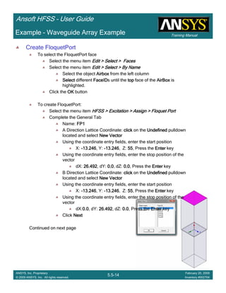
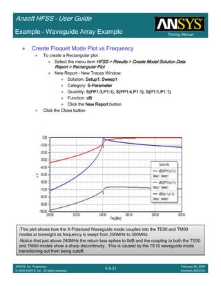
•Notice the transmission for the 1st Floquet Mode is not significant until just below 30deg scan.
This mode corresponds to the TM0-1 mode which doesn’t propagate until 29deg scan. At this
same scan angle a scan blindness is observed in the return loss and the transmission for the
4th Floquet Mode (TM00) drops sharply.
0.00 10.00 20.00 30.00 40.00 50.00 60.00 70.00 80.00 90.00
theta_scan [deg]
0.00
0.10
0.20
0.30
0.40
0.50
0.60
0.70
0.80
0.90
1.00
Y1
Ansoft Corporation HFSSDesign1XY Plot 5
Curve Info
mag(S(FP1:2,p1:1))
Setup2 : LastAdaptive
Freq='0.29979GHz'
mag(S(FP1:4,p1:1))
Setup2 : LastAdaptive
Freq='0.29979GHz'
mag(S(p1:1,p1:1))
Setup2 : LastAdaptive
Freq='0.29979GHz'](https://image.slidesharecdn.com/hfssuser-guide-150114060507-conversion-gate02/85/Hfss-user-guide-274-320.jpg)
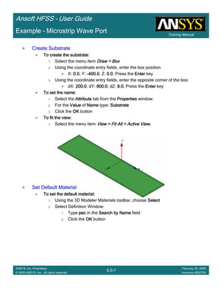
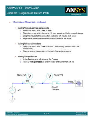
![Training Manual
Ansoft HFSS – User Guide
5.5-27
ANSYS, Inc. Proprietary
© 2009 ANSYS, Inc. All rights reserved.
February 20, 2009
Inventory #002704
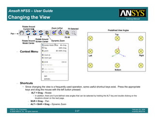
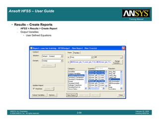
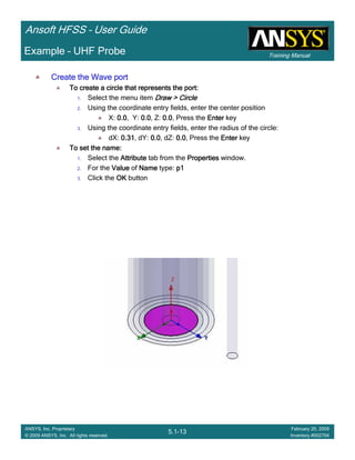
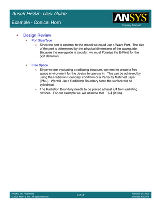
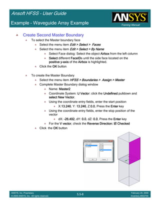
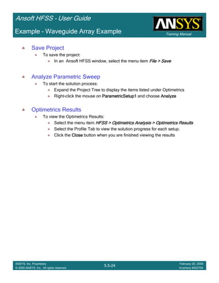
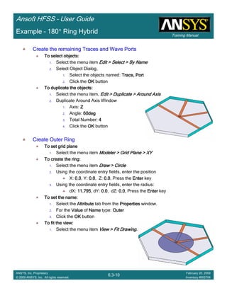
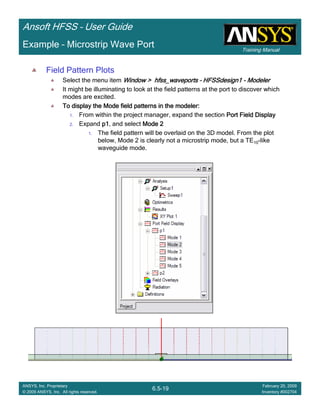
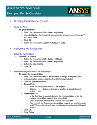
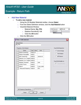
Example – Waveguide Array Example
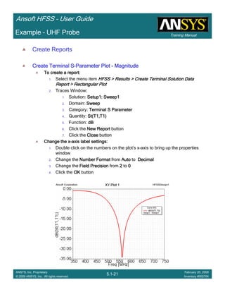
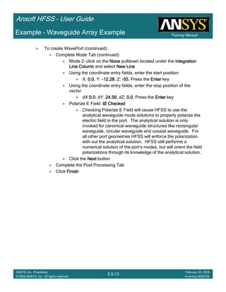
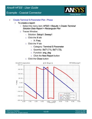
Create Active Element Pattern
To create a report:
Select the menu item HFSS > Results > Create Modal Solution DataHFSS > Results > Create Modal Solution DataHFSS > Results > Create Modal Solution DataHFSS > Results > Create Modal Solution Data
Report > Rectangular PlotReport > Rectangular PlotReport > Rectangular PlotReport > Rectangular Plot
Traces Window:
Solution: Setup2: LastAdaptiveSetup2: LastAdaptiveSetup2: LastAdaptiveSetup2: LastAdaptive
X: Switch to theta_scantheta_scantheta_scantheta_scan
Y:
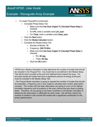
10*log(4*pi*701.8/39.361^2*mag(S(p1:2,FP1:4))^2*cos(theta_scan))10*log(4*pi*701.8/39.361^2*mag(S(p1:2,FP1:4))^2*cos(theta_scan))10*log(4*pi*701.8/39.361^2*mag(S(p1:2,FP1:4))^2*cos(theta_scan))10*log(4*pi*701.8/39.361^2*mag(S(p1:2,FP1:4))^2*cos(theta_scan))
701.8 is the unit cell area in square inches
39.361inches is the wavelength in free space
Click the New ReportNew ReportNew ReportNew Report button
Click the CloseCloseCloseClose button
Double click on the Y-axis of the plot
Click the Scale tab:
Specify Min: CheckedCheckedCheckedChecked
Min: ----60606060
Spacing: 10101010
0.00 10.00 20.00 30.00 40.00 50.00 60.00 70.00 80.00 90.00
theta_scan [deg]
-60.00
-50.00
-40.00
-30.00
-20.00
-10.00
0.00
10.00
20.00
10*log(4*pi*701.8/39.361^2*mag(S(p1:1,FP1:4))^2*cos(theta_scan))
Ansoft Corporation HFSSDesign1XY Plot 6
Curve Info
10*log(4*pi*701.8/39.361^2*mag(S(p1:1,FP1:4))^2*cos(theta_scan))
Setup2 : LastAdaptive
Freq='0.29979GHz'](https://image.slidesharecdn.com/hfssuser-guide-150114060507-conversion-gate02/85/Hfss-user-guide-275-320.jpg)


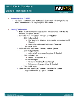

![Training Manual
Ansoft HFSS – User Guide
7.1-20
ANSYS, Inc. Proprietary
© 2009 ANSYS, Inc. All rights reserved.
February 20, 2009
Inventory #002704
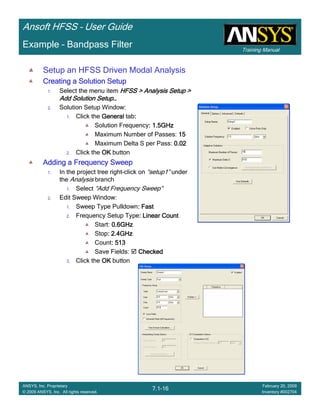
Example – Bandpass Filter
0.60 0.80 1.00 1.20 1.40 1.60 1.80 2.00 2.20 2.40
Freq [GHz]
-70.00
-60.00
-50.00
-40.00
-30.00
-20.00
-10.00
0.00
Y1
Ansoft Corporation HFSSDesign1XY Plot 1
Curve Info
dB(S(p1,p1))
Setup1 : Sweep1
dB(S(p2,p1))
Setup1 : Sweep1
Note new plot “XY Plot 1” in project
tree](https://image.slidesharecdn.com/hfssuser-guide-150114060507-conversion-gate02/85/Hfss-user-guide-434-320.jpg)
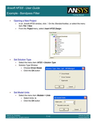
![Training Manual
Ansoft HFSS – User Guide
7.1-22
ANSYS, Inc. Proprietary
© 2009 ANSYS, Inc. All rights reserved.
February 20, 2009
Inventory #002704
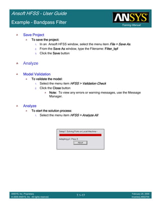
Example – Bandpass Filter
Rename PlotRename PlotRename PlotRename Plot
In the Project tree right-click on the branch HFSSDesign1 > Results > XY Plot 1HFSSDesign1 > Results > XY Plot 1HFSSDesign1 > Results > XY Plot 1HFSSDesign1 > Results > XY Plot 1
Select Rename
Change name to S-params
<return>
0.60 0.80 1.00 1.20 1.40 1.60 1.80 2.00 2.20 2.40
Freq [GHz]
-60.00
-50.00
-40.00
-30.00
-20.00
-10.00
0.00
dB(S(p1,p1))
-1.00
-0.90
-0.80
-0.70
-0.60
-0.50
-0.40
-0.30
-0.20
-0.10
0.00
dB(S(p2,p1))
Ansoft Corporation HFSSDesign1S-params
Curve Info
dB(S(p1,p1))
Setup1 : Sweep1
dB(S(p2,p1))
Setup1 : Sweep1](https://image.slidesharecdn.com/hfssuser-guide-150114060507-conversion-gate02/85/Hfss-user-guide-436-320.jpg)

![Training Manual
Ansoft HFSS – User Guide
8.1-19
ANSYS, Inc. Proprietary
© 2009 ANSYS, Inc. All rights reserved.
February 20, 2009
Inventory #002704
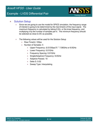
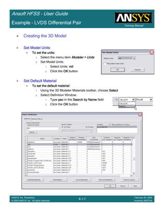
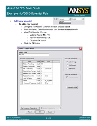
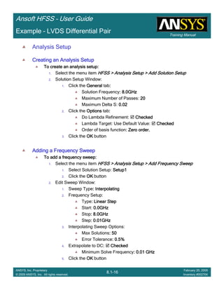
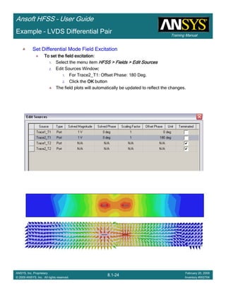
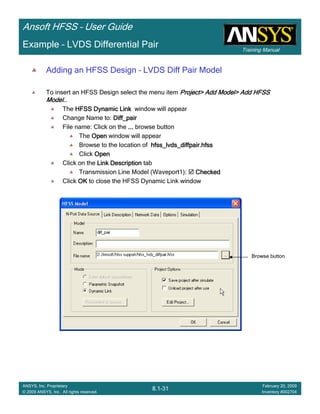
Example – LVDS Differential Pair
0.00 1.00 2.00 3.00 4.00 5.00 6.00 7.00 8.00
Freq [GHz]
-100.00
-80.00
-60.00
-40.00
-20.00
0.00
Y1
Ansoft Corporation HFSSModel1XY Plot 1
Curve Info
dB(St(Diff1,Diff1))
Setup1 : Sweep1
dB(St(Diff1,Comm1))
Setup1 : Sweep1
dB(St(Diff1,p2_Diff1))
Setup1 : Sweep1
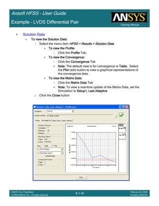
Create Reports
Create Differential Pair SCreate Differential Pair SCreate Differential Pair SCreate Differential Pair S----Parameter PlotParameter PlotParameter PlotParameter Plot
To create a report:To create a report:To create a report:To create a report:
1. Select the menu item HFSS > Results > Create Terminal Solution DataHFSS > Results > Create Terminal Solution DataHFSS > Results > Create Terminal Solution DataHFSS > Results > Create Terminal Solution Data
Report > Rectangular PlotReport > Rectangular PlotReport > Rectangular PlotReport > Rectangular Plot
2. Context Window:
1. Solution: Setup1: Sweep1Setup1: Sweep1Setup1: Sweep1Setup1: Sweep1
2. Domain: SweepSweepSweepSweep
3. Trace Window
1. Category: Terminal S ParametersTerminal S ParametersTerminal S ParametersTerminal S Parameters
2. Quantity: St(Diff1,Diff1), St(Diff1,Comm1), St(Diff1, Diff2St(Diff1,Diff1), St(Diff1,Comm1), St(Diff1, Diff2St(Diff1,Diff1), St(Diff1,Comm1), St(Diff1, Diff2St(Diff1,Diff1), St(Diff1,Comm1), St(Diff1, Diff2)
3. Function: dBdBdBdB
4. Click the New ReportNew ReportNew ReportNew Report button
5. Click the CloseCloseCloseClose button](https://image.slidesharecdn.com/hfssuser-guide-150114060507-conversion-gate02/85/Hfss-user-guide-457-320.jpg)
![Training Manual
Ansoft HFSS – User Guide
8.1-28
ANSYS, Inc. Proprietary
© 2009 ANSYS, Inc. All rights reserved.
February 20, 2009
Inventory #002704
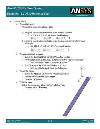
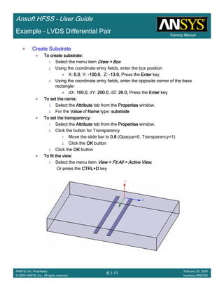
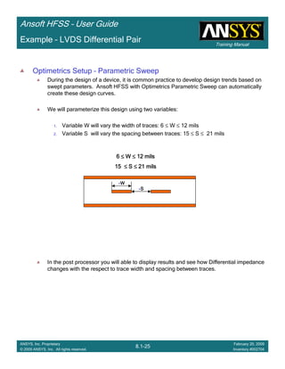
Example – LVDS Differential Pair
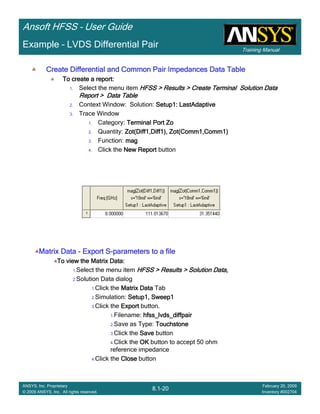
Create Reports
Create Terminal Port Zo vs SCreate Terminal Port Zo vs SCreate Terminal Port Zo vs SCreate Terminal Port Zo vs S
To Create a report:To Create a report:To Create a report:To Create a report:
1. Select the menu item HFSS > Results > Create Terminal Solution DataHFSS > Results > Create Terminal Solution DataHFSS > Results > Create Terminal Solution DataHFSS > Results > Create Terminal Solution Data
Report >Report >Report >Report > Rectangular PlotRectangular PlotRectangular PlotRectangular Plot
2. Context Window:
1. Solution: Setup1: LastAdaptiveSetup1: LastAdaptiveSetup1: LastAdaptiveSetup1: LastAdaptive
3. Trace Window
1. X: S
2. Category: Terminal Port ZoTerminal Port ZoTerminal Port ZoTerminal Port Zo
3. Quantity: Zot(Diff1,Diff1), Zot(Comm1,Comm1)Zot(Diff1,Diff1), Zot(Comm1,Comm1)Zot(Diff1,Diff1), Zot(Comm1,Comm1)Zot(Diff1,Diff1), Zot(Comm1,Comm1)
4. Function: MagMagMagMag
5. Click the New ReportNew ReportNew ReportNew Report button
6. Click the CloseCloseCloseClose button
15.00 16.00 17.00 18.00 19.00 20.00 21.00
S[mil]
0.00
20.00
40.00
60.00
80.00
100.00
120.00
Y1
Ansoft Corporation HFSSDesign1XYPlot 3
CurveInfo
mag(Zot(Comm1,C
Setup1: LastAdaptive
Freq='8GHz' W='6mil'
mag(Zot(Comm1,C
Setup1: LastAdaptive
Freq='8GHz' W='9mil'
mag(Zot(Comm1,C
Setup1: LastAdaptive
Freq='8GHz' W='12mil'
mag(Zot(Diff1,Diff1
Setup1: LastAdaptive
Freq='8GHz' W='6mil'
mag(Zot(Diff1,Diff1
Setup1: LastAdaptive
Freq='8GHz' W='9mil'
mag(Zot(Diff1,Diff1
Setup1: LastAdaptive
Freq='8GHz' W='12mil'](https://image.slidesharecdn.com/hfssuser-guide-150114060507-conversion-gate02/85/Hfss-user-guide-466-320.jpg)


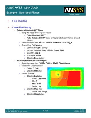
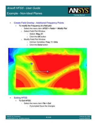
![Training Manual
Ansoft HFSS – User Guide
8.3-22
ANSYS, Inc. Proprietary
© 2009 ANSYS, Inc. All rights reserved.
February 20, 2009
Inventory #002704
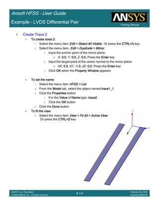
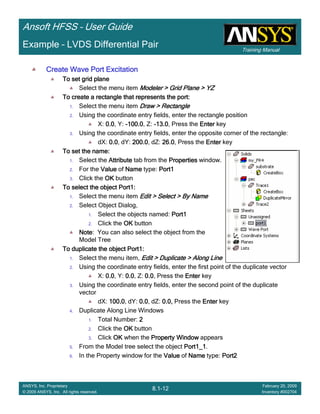
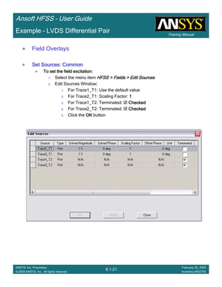
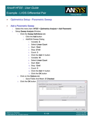
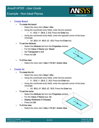
Example – Non-Ideal Planes
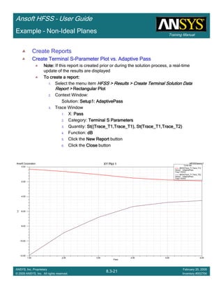
CreateCreateCreateCreate TerminalTerminalTerminalTerminal S Plot vs FrequencyS Plot vs FrequencyS Plot vs FrequencyS Plot vs Frequency
To create a report:To create a report:To create a report:To create a report:
1. Select the menu item HFSS > Results > Create Terminal Solution DataHFSS > Results > Create Terminal Solution DataHFSS > Results > Create Terminal Solution DataHFSS > Results > Create Terminal Solution Data
Report >Report >Report >Report > Rectangular PlotRectangular PlotRectangular PlotRectangular Plot
2. Context Window:
1. Solution: Setup1: Sweep1Setup1: Sweep1Setup1: Sweep1Setup1: Sweep1
2. Domain: SweepSweepSweepSweep
3. Trace Window
1. Category: Terminal S ParametersTerminal S ParametersTerminal S ParametersTerminal S Parameters
2. Quantity: St(Trace_T1,Trace_T1), St(Trace_T1,Trace_T2)St(Trace_T1,Trace_T1), St(Trace_T1,Trace_T2)St(Trace_T1,Trace_T1), St(Trace_T1,Trace_T2)St(Trace_T1,Trace_T1), St(Trace_T1,Trace_T2)
3. Function: dBdBdBdB
4. Click the New ReportNew ReportNew ReportNew Report button
5. Click the CloseCloseCloseClose button
To add data marker to the PlotsTo add data marker to the PlotsTo add data marker to the PlotsTo add data marker to the Plots
1. Select the menu item Report2D > Marker > Add MarkerReport2D > Marker > Add MarkerReport2D > Marker > Add MarkerReport2D > Marker > Add Marker
2. Move cursor to the resonant points on the plotting curve and click the left
mouse button
3. When you are finished placing markers at the resonances, Press ESCESCESCESC Or
right-click the mouse and select Exit Marker ModeExit Marker ModeExit Marker ModeExit Marker Mode.
0.00 1.00 2.00 3.00 4.00 5.00 6.00 7.00 8.00 9.00 10.00
Freq [GHz]
-50.00
-40.00
-30.00
-20.00
-10.00
0.00
Y1
Ansoft Corporation HFSSDesign1XY Plot 2
m1
m2
m3
m4 m5
m6
Curve Info
dB(St(Trace_T1,Trace_T1))
Setup1 : Sweep1
dB(St(Trace_T1,Trace_T2))
Setup1 : Sweep1
Name X Y
m1 1.7700 -40.0894
m2 4.2900 -36.3371
m3 5.2500 -49.4293
m4 7.1200 -45.5499
m5 7.5100 -46.0011
m6 8.0900 -21.9133](https://image.slidesharecdn.com/hfssuser-guide-150114060507-conversion-gate02/85/Hfss-user-guide-538-320.jpg)


![Training Manual
Ansoft HFSS – User Guide
8.4-20
ANSYS, Inc. Proprietary
© 2009 ANSYS, Inc. All rights reserved.
February 20, 2009
Inventory #002704
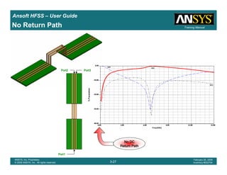
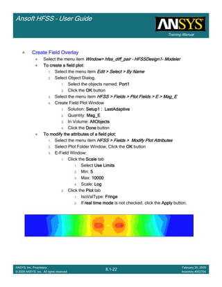
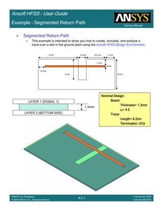
Example – Return Path
0.00 2.00 4.00 6.00 8.00 10.00 12.00 14.00 16.00
Freq [GHz]
-40.00
-35.00
-30.00
-25.00
-20.00
-15.00
-10.00
-5.00
0.00
Y1
Ansoft Corporation HFSSDesign1XY Plot 2
Curve Info
dB(St(Cond_T1,Cond_T1))
Setup1 : Sweep1
dB(St(Cond_T1,Cond_T2))
Setup1 : Sweep1
dB(St(Cond_T1,Cond_T3))
Setup1 : Sweep1
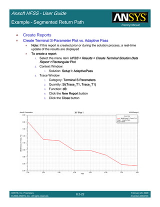
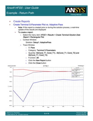
Create TerminalCreate TerminalCreate TerminalCreate Terminal SSSS----Parameter Plot vs FrequencyParameter Plot vs FrequencyParameter Plot vs FrequencyParameter Plot vs Frequency
1. Select the menu item HFSS > Results > Create Terminal Solution DataHFSS > Results > Create Terminal Solution DataHFSS > Results > Create Terminal Solution DataHFSS > Results > Create Terminal Solution Data
Report >Report >Report >Report > Rectangular PlotRectangular PlotRectangular PlotRectangular Plot
2. Context Window:
1. Solution: Setup1: Sweep1Setup1: Sweep1Setup1: Sweep1Setup1: Sweep1
2. Domain: SweepSweepSweepSweep
3. Trace Window
1. Category: Terminal S ParametersTerminal S ParametersTerminal S ParametersTerminal S Parameters
2. Quantity: St(Cond_T1, Cond_T1) , St(Cond_T1, Cond_T2) andSt(Cond_T1, Cond_T1) , St(Cond_T1, Cond_T2) andSt(Cond_T1, Cond_T1) , St(Cond_T1, Cond_T2) andSt(Cond_T1, Cond_T1) , St(Cond_T1, Cond_T2) and
St(Cond_T1, Cond_T3)St(Cond_T1, Cond_T3)St(Cond_T1, Cond_T3)St(Cond_T1, Cond_T3)
3. Function: dBdBdBdB
4. Click the New ReportNew ReportNew ReportNew Report button
5. Click the CloseCloseCloseClose button
No DCNo DCNo DCNo DC
Return PathReturn PathReturn PathReturn Path](https://image.slidesharecdn.com/hfssuser-guide-150114060507-conversion-gate02/85/Hfss-user-guide-560-320.jpg)
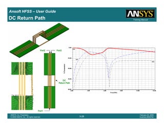
![Training Manual
Ansoft HFSS – User Guide
8.4-24
ANSYS, Inc. Proprietary
© 2009 ANSYS, Inc. All rights reserved.
February 20, 2009
Inventory #002704
Example – Return Path
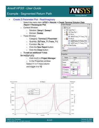
Save ProjectSave ProjectSave ProjectSave Project
To save the project:To save the project:To save the project:To save the project:
1. In an Ansoft HFSS window, select the menu item File > SaveFile > SaveFile > SaveFile > Save
Analyze
Model ValidationModel ValidationModel ValidationModel Validation
To validate the model:To validate the model:To validate the model:To validate the model:
1. Select the menu item HFSS > Validation CheckHFSS > Validation CheckHFSS > Validation CheckHFSS > Validation Check
2. Click the CloseCloseCloseClose button
AnalyzeAnalyzeAnalyzeAnalyze
To start the solution process:To start the solution process:To start the solution process:To start the solution process:
1. Select the menu item HFSS > Analyze AllHFSS > Analyze AllHFSS > Analyze AllHFSS > Analyze All
To Open All Existing ReportTo Open All Existing ReportTo Open All Existing ReportTo Open All Existing Report
To open all reports:To open all reports:To open all reports:To open all reports:
1. Select the menu item HFSS > Results > Open All ReportsHFSS > Results > Open All ReportsHFSS > Results > Open All ReportsHFSS > Results > Open All Reports
0.00 2.00 4.00 6.00 8.00 10.00 12.00 14.00 16.00
Freq [GHz]
-45.00
-40.00
-35.00
-30.00
-25.00
-20.00
-15.00
-10.00
-5.00
0.00
Y1
Ansoft Corporation HFSSDesign2XY Plot 2
Curve Info
dB(St(Cond_T1,Cond_T1))
Setup1 : Sweep1
dB(St(Cond_T1,Cond_T2))
Setup1 : Sweep1
dB(St(Cond_T1,Cond_T3))
Setup1 : Sweep1](https://image.slidesharecdn.com/hfssuser-guide-150114060507-conversion-gate02/85/Hfss-user-guide-564-320.jpg)
![Training Manual
Ansoft HFSS – User Guide
8.4-28
ANSYS, Inc. Proprietary
© 2009 ANSYS, Inc. All rights reserved.
February 20, 2009
Inventory #002704
Example – Return Path
Save ProjectSave ProjectSave ProjectSave Project
To save the project:To save the project:To save the project:To save the project:
1. In an Ansoft HFSS window, select the menu item File > SaveFile > SaveFile > SaveFile > Save
Analyze
Model ValidationModel ValidationModel ValidationModel Validation
To validate the model:To validate the model:To validate the model:To validate the model:
1. Select the menu item HFSS > Validation CheckHFSS > Validation CheckHFSS > Validation CheckHFSS > Validation Check
2. Click the CloseCloseCloseClose button
AnalyzeAnalyzeAnalyzeAnalyze
To start the solution process:To start the solution process:To start the solution process:To start the solution process:
1. Select the menu item HFSS > AnalyzeHFSS > AnalyzeHFSS > AnalyzeHFSS > Analyze
To Open All Existing ReportTo Open All Existing ReportTo Open All Existing ReportTo Open All Existing Report
To open all reports:To open all reports:To open all reports:To open all reports:
1. Select the menu item HFSS > Results > Open All ReportsHFSS > Results > Open All ReportsHFSS > Results > Open All ReportsHFSS > Results > Open All Reports
Exiting HFSSExiting HFSSExiting HFSSExiting HFSS
To Exit HFSS:To Exit HFSS:To Exit HFSS:To Exit HFSS:
1. Select the menu item File > ExitFile > ExitFile > ExitFile > Exit
1. If prompted Save the changes
0.00 5.00 10.00 15.00
Freq[GHz]
-60.00
-50.00
-40.00
-30.00
-20.00
-10.00
0.00
Y1
Ansoft Corporation HFSSDesign4XYPlot 2
CurveInfo
dB(St(Cond_T1,Cond_T1))
Setup1: Sweep1
dB(St(Cond_T1,Cond_T2))
Setup1: Sweep1
dB(St(Cond_T1,Cond_T3))
Setup1: Sweep1](https://image.slidesharecdn.com/hfssuser-guide-150114060507-conversion-gate02/85/Hfss-user-guide-568-320.jpg)


![Training Manual
Ansoft HFSS – User Guide
9.1-27
ANSYS, Inc. Proprietary
© 2009 ANSYS, Inc. All rights reserved.
February 20, 2009
Inventory #002704
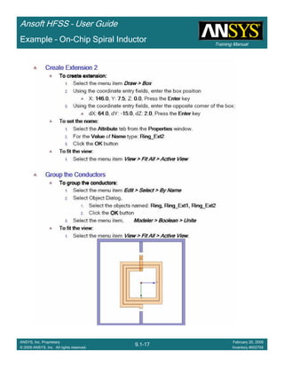
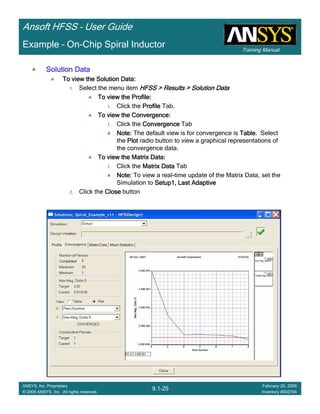
Example – On-Chip Spiral Inductor
0.00 5.00 10.00 15.00 20.00
Freq [GHz]
0.00
1.00
2.00
3.00
4.00
5.00
6.00
7.00
8.00
9.00
Y1
Ansoft Corporation HFSSDesign1Q Plot
Curve Info
abs(Q11)
Setup1 : Sweep1
abs(Q22)
Setup1 : Sweep1
Custom EquationsCustom EquationsCustom EquationsCustom Equations –––– Output VariablesOutput VariablesOutput VariablesOutput Variables
Select the menu item HFSS > Results > Create Terminal Solution Data Report >HFSS > Results > Create Terminal Solution Data Report >HFSS > Results > Create Terminal Solution Data Report >HFSS > Results > Create Terminal Solution Data Report >
Rectangular PlotRectangular PlotRectangular PlotRectangular Plot
Trace Window
1.1.1.1. Click the Output VariablesOutput VariablesOutput VariablesOutput Variables button
2. Output Variables dialog
1. Name: Q11Q11Q11Q11
2. Expression:
1. Category: Terminal Y ParametersTerminal Y ParametersTerminal Y ParametersTerminal Y Parameters
2. Quantity: Yt(1,1)Yt(1,1)Yt(1,1)Yt(1,1)
3. Function: imimimim
4. Click the Insert into ExpressionInsert into ExpressionInsert into ExpressionInsert into Expression button
5. Type: ////
6. Quantity: Yt(1,1)Yt(1,1)Yt(1,1)Yt(1,1)
7. Function: rererere
8. Click the Insert into ExpressionInsert into ExpressionInsert into ExpressionInsert into Expression button
3. Click the AddAddAddAdd button
4. Repeat for Q22Q22Q22Q22, by replacing Yt(1,1)Yt(1,1)Yt(1,1)Yt(1,1) with Yt(2,2)Yt(2,2)Yt(2,2)Yt(2,2)
3. Solution: Setup1: Sweep1Setup1: Sweep1Setup1: Sweep1Setup1: Sweep1
4. Domain: SweepSweepSweepSweep
5. Click YYYY tab
Category: Output VariablesOutput VariablesOutput VariablesOutput Variables
Quantity: Q11, Q22Q11, Q22Q11, Q22Q11, Q22
Function: absabsabsabs
Click the New ReportNew ReportNew ReportNew Report button
6. Click the CloseCloseCloseClose button](https://image.slidesharecdn.com/hfssuser-guide-150114060507-conversion-gate02/85/Hfss-user-guide-595-320.jpg)


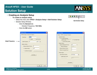
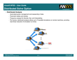
This document provides an introduction and overview of the Ansoft HFSS simulation software. It discusses what HFSS is used for, how to install it, how to get help, and defines key terms related to using the HFSS interface and building models. Specifically, it explains that HFSS is an electromagnetic field simulation software that uses finite element analysis. It also reviews the main sections of the interface like the project manager, property window, and 3D modeler window.


![High_Frequency_Structure_Simulator_HFSS[1].pdf](https://cdn.slidesharecdn.com/ss_thumbnails/highfrequencystructuresimulatorhfss1-250707201635-2208bc58-thumbnail.jpg?width=640&height=640&fit=bounds)


![Polymer [ बहुलक ] Chemistry Notes PDF - Irfanullah Mehar - JJ Sir Chemistry.pdf](https://cdn.slidesharecdn.com/ss_thumbnails/polymerchemistrynotespdf-irfanullahmehar-jjsirchemistry-260210172118-3f9b37f7-thumbnail.jpg?width=640&height=640&fit=bounds)


