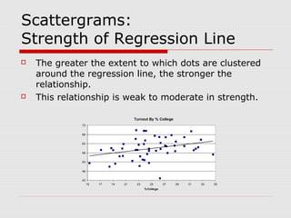
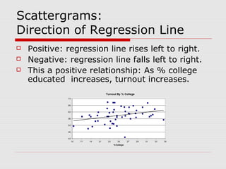
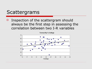
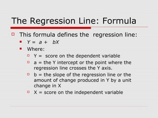
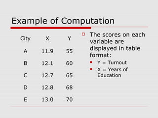
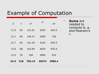
Chapter 15


  Association Between Variables
  Measured at the Interval-Ratio
  Level
Chapter Outline
   Interpreting the Correlation
    Coefficient: r 2
   The Correlation Matrix
   Testing Pearson’s r for Significance
   Interpreting Statistics: The Correlates
    of Crime
Scattergrams
   Scattergrams have two dimensions:
       The X (independent) variable is arrayed
        along the horizontal axis.
       The Y (dependent) variable is arrayed
        along the vertical axis.
Scattergrams
   Each dot on a scattergram is a case.
   The dot is placed at the intersection
    of the case’s scores on X and Y.
Scattergra ms
   Shows the relationship between %
    College Educated (X) and Voter Turnout
    (Y) on election day for the 50 states.
                                Turnout By % College
       73


       68


       63


       58


       53


       48


       43
            15   17   19   21    23      25       27   29   31   33   35
                                      % College
Scattergrams
   Horizontal X axis - % of population of a
    state with a college education.
      Scores range from 15.3% to 34.6%
       and increase from left to right.
                                 Turnout By % College
        73


        68


        63


        58


        53


        48


        43
             15   17   19   21    23      25       27   29   31   33   35
                                       % College
Scattergrams
   Vertical (Y) axis is voter turnout.
     Scores range from 44.1% to 70.4% and
      increase from bottom to top
                                Turnout By % College
       73


       68


       63


       58


       53


       48


       43
            15   17   19   21    23      25       27   29   31   33   35
                                      % College
Scattergrams: Regression Line
   A single straight line that comes as close as
    possible to all data points.
   Indicates strength and direction of the
    relationship.
                                 Turnout By % College
        73


        68


        63


        58


        53


        48


        43
             15   17   19   21    23      25       27   29   31   33   35
                                       % College
Scattergrams:
Strength of Regression Line
   The greater the extent to which dots are clustered
    around the regression line, the stronger the
    relationship.
   This relationship is weak to moderate in strength.

                                       Turnout By % College
              73


              68


              63


              58


              53


              48


              43
                   15   17   19   21    23      25       27   29   31   33   35
                                             % College
Scattergrams:
Direction of Regression Line
   Positive: regression line rises left to right.
   Negative: regression line falls left to right.
   This a positive relationship: As % college
    educated increases, turnout increases.
                                       Turnout By % College
              73


              68


              63


              58


              53


              48


              43
                   15   17   19   21    23      25       27   29   31   33   35
                                             % College
Scattergrams
   Inspection of the scattergram should
    always be the first step in assessing the
    correlation between two I-R variables
                                  Turnout By % College
         73


         68


         63


         58


         53


         48


         43
              15   17   19   21    23      25       27   29   31   33   35
                                        % College
The Regression Line: Formula
   This formula defines the regression line:
       Y = a + bX
       Where:
          Y = score on the dependent variable
          a = the Y intercept or the point where the
           regression line crosses the Y axis.
          b = the slope of the regression line or the
           amount of change produced in Y by a unit
           change in X
          X = score on the independent variable
Regression Analysis
   Before using the formula for the regression line, a
    and b must be calculated.
   Compute b first, using Formula 15.3 (we won’t do
    any calculation for this chapter)
Regression Analysis
   The Y intercept (a) is computed from
    Formula 15.4:
Regression Analysis
   For the relationship between % college
    educated and turnout:
       b (slope) = .42
       a (Y intercept)= 50.03
   Regression formula: Y = 50.03 + .42 X
   A slope of .42 means that turnout increases
    by .42 (less than half a percent) for every
    unit increase of 1 in % college educated.
   The Y intercept means that the regression
    line crosses the Y axis at Y = 50.03.
Predicting Y
   What turnout would be expected in a state
    where only 10% of the population was
    college educated?
   What turnout would be expected in a state
    where 70% of the population was college
    educated?
   This is a positive relationship so the value
    for Y increases as X increases:
       For X =10, Y = 50.3 +.42(10) = 54.5
       For X =70, Y = 50.3 + .42(70) = 79.7
Pearson correlation coefficient
   But of course, this is just an estimate of
    turnout based on % college educated, and
    many other factors also affect voter
    turnout.
   How much of the variation in voter turnout
    depends on % college educated? The
    relevant statististic is the coefficient of
    determination (r squared), but first we
    need to learn about Pearson’s correlation
    coefficient (r).
Pearson’s r
   Pearson’s r is a measure of association for I-R
    variables.
   It varies from -1.0 to +1.0
   Relationship may be positive (as X increases, Y
    increases) or negative (as X increases, Y decreases)
   For the relationship between % college educated and
    turnout, r =.32.
   The relationship is positive: as level of education
    increases, turnout increases.
   How strong is the relationship? For that we use R
    squared, but first, let’s look at the calculation process
Example of Computation
   The computation and interpretation of a, b,
    and Pearson’s r will be illustrated using
    Problem 15.1.
   The variables are:
       Voter turnout (Y)
       Average years of school (X)
   The sample is 5 cities.
       This is only to simplify computations, 5 is much
        too small a sample for serious research.
Example of Computation
                       The scores on each
 City    X     Y
                        variable are
  A     11.9   55
                        displayed in table
                        format:
  B     12.1   60          Y = Turnout
                           X = Years of
  C     12.7   65           Education

  D     12.8   68

  E     13.0   70
Example of Computation
                        Y2
                                           Sums are
  X      Y      X2
                                 XY         needed to
                                            compute b, a,
 11.9   55    141.61   3025    654.5        and Pearson’s
                                            r.
 12.1   60    146.41   3600     726

 12.7   65    161.29   4225    825.5

 12.8   68    163.84   4624    870.4

 13.0   70     169     4900     910

 62.5   318   782.15   20374   3986.4
Interpreting Pearson’s r
   An r of 0.98 indicates an extremely strong
    relationship between average years of
    education and voter turnout for these five
    cities.
   The coefficient of determination is r2 = .96.
    Knowing education level improves our
    prediction of voter turnout by 96%. This is
    a PRE measure (like lambda and gamma)
   We could also say that education explains
    96% of the variation in voter turnout.
Interpreting Pearson’s r
   Our first example provides a more
    realistic value for r.
       The r between turnout and % college
        educated for the 50 states was:
           r = .32
           This is a weak to moderate, positive
            relationship.
   The value of r2 is .10.
    Percent college educated explains
    10% of the variation in turnout.

Healey ch15b

  • 1.
    Chapter 15 Association Between Variables Measured at the Interval-Ratio Level
  • 2.
    Chapter Outline  Interpreting the Correlation Coefficient: r 2  The Correlation Matrix  Testing Pearson’s r for Significance  Interpreting Statistics: The Correlates of Crime
  • 3.
    Scattergrams  Scattergrams have two dimensions:  The X (independent) variable is arrayed along the horizontal axis.  The Y (dependent) variable is arrayed along the vertical axis.
  • 4.
    Scattergrams  Each dot on a scattergram is a case.  The dot is placed at the intersection of the case’s scores on X and Y.
  • 5.
    Scattergra ms  Shows the relationship between % College Educated (X) and Voter Turnout (Y) on election day for the 50 states. Turnout By % College 73 68 63 58 53 48 43 15 17 19 21 23 25 27 29 31 33 35 % College
  • 6.
    Scattergrams  Horizontal X axis - % of population of a state with a college education.  Scores range from 15.3% to 34.6% and increase from left to right. Turnout By % College 73 68 63 58 53 48 43 15 17 19 21 23 25 27 29 31 33 35 % College
  • 7.
    Scattergrams  Vertical (Y) axis is voter turnout.  Scores range from 44.1% to 70.4% and increase from bottom to top Turnout By % College 73 68 63 58 53 48 43 15 17 19 21 23 25 27 29 31 33 35 % College
  • 8.
    Scattergrams: Regression Line  A single straight line that comes as close as possible to all data points.  Indicates strength and direction of the relationship. Turnout By % College 73 68 63 58 53 48 43 15 17 19 21 23 25 27 29 31 33 35 % College
  • 9.
    Scattergrams: Strength of RegressionLine  The greater the extent to which dots are clustered around the regression line, the stronger the relationship.  This relationship is weak to moderate in strength. Turnout By % College 73 68 63 58 53 48 43 15 17 19 21 23 25 27 29 31 33 35 % College
  • 10.
    Scattergrams: Direction of RegressionLine  Positive: regression line rises left to right.  Negative: regression line falls left to right.  This a positive relationship: As % college educated increases, turnout increases. Turnout By % College 73 68 63 58 53 48 43 15 17 19 21 23 25 27 29 31 33 35 % College
  • 11.
    Scattergrams  Inspection of the scattergram should always be the first step in assessing the correlation between two I-R variables Turnout By % College 73 68 63 58 53 48 43 15 17 19 21 23 25 27 29 31 33 35 % College
  • 12.
    The Regression Line:Formula  This formula defines the regression line:  Y = a + bX  Where:  Y = score on the dependent variable  a = the Y intercept or the point where the regression line crosses the Y axis.  b = the slope of the regression line or the amount of change produced in Y by a unit change in X  X = score on the independent variable
  • 13.
    Regression Analysis  Before using the formula for the regression line, a and b must be calculated.  Compute b first, using Formula 15.3 (we won’t do any calculation for this chapter)
  • 14.
    Regression Analysis  The Y intercept (a) is computed from Formula 15.4:
  • 15.
    Regression Analysis  For the relationship between % college educated and turnout:  b (slope) = .42  a (Y intercept)= 50.03  Regression formula: Y = 50.03 + .42 X  A slope of .42 means that turnout increases by .42 (less than half a percent) for every unit increase of 1 in % college educated.  The Y intercept means that the regression line crosses the Y axis at Y = 50.03.
  • 16.
    Predicting Y  What turnout would be expected in a state where only 10% of the population was college educated?  What turnout would be expected in a state where 70% of the population was college educated?  This is a positive relationship so the value for Y increases as X increases:  For X =10, Y = 50.3 +.42(10) = 54.5  For X =70, Y = 50.3 + .42(70) = 79.7
  • 17.
    Pearson correlation coefficient  But of course, this is just an estimate of turnout based on % college educated, and many other factors also affect voter turnout.  How much of the variation in voter turnout depends on % college educated? The relevant statististic is the coefficient of determination (r squared), but first we need to learn about Pearson’s correlation coefficient (r).
  • 18.
    Pearson’s r  Pearson’s r is a measure of association for I-R variables.  It varies from -1.0 to +1.0  Relationship may be positive (as X increases, Y increases) or negative (as X increases, Y decreases)  For the relationship between % college educated and turnout, r =.32.  The relationship is positive: as level of education increases, turnout increases.  How strong is the relationship? For that we use R squared, but first, let’s look at the calculation process
  • 19.
    Example of Computation  The computation and interpretation of a, b, and Pearson’s r will be illustrated using Problem 15.1.  The variables are:  Voter turnout (Y)  Average years of school (X)  The sample is 5 cities.  This is only to simplify computations, 5 is much too small a sample for serious research.
  • 20.
    Example of Computation  The scores on each City X Y variable are A 11.9 55 displayed in table format: B 12.1 60  Y = Turnout  X = Years of C 12.7 65 Education D 12.8 68 E 13.0 70
  • 21.
    Example of Computation Y2  Sums are X Y X2 XY needed to compute b, a, 11.9 55 141.61 3025 654.5 and Pearson’s r. 12.1 60 146.41 3600 726 12.7 65 161.29 4225 825.5 12.8 68 163.84 4624 870.4 13.0 70 169 4900 910 62.5 318 782.15 20374 3986.4
  • 22.
    Interpreting Pearson’s r  An r of 0.98 indicates an extremely strong relationship between average years of education and voter turnout for these five cities.  The coefficient of determination is r2 = .96. Knowing education level improves our prediction of voter turnout by 96%. This is a PRE measure (like lambda and gamma)  We could also say that education explains 96% of the variation in voter turnout.
  • 23.
    Interpreting Pearson’s r  Our first example provides a more realistic value for r.  The r between turnout and % college educated for the 50 states was:  r = .32  This is a weak to moderate, positive relationship.  The value of r2 is .10. Percent college educated explains 10% of the variation in turnout.