Downloaded 59 times

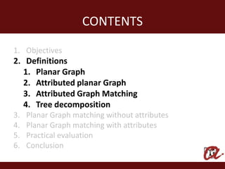
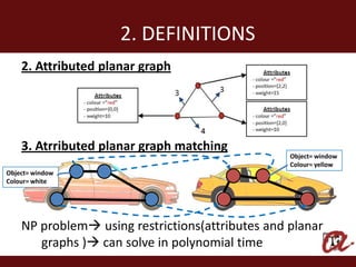
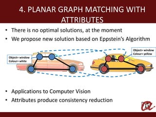
![4. PLANAR GRAPH MATCHING WITH
ATTRIBUTES
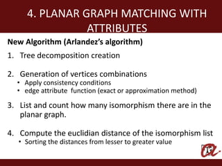
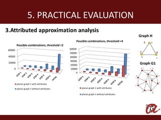
New Algorithm (Arlandez’s algorithm) Graph H
• Euclidian distance 1
Planar graph 2 2
1
3
# A D F G E x y C B H Euclidian distance
1 [] a [] d b [] [] c [] [] 0
2 [] a c d [] [] [] [] b [] 0
3 [] d [] a b [] [] c [] [] 0
4 [] d c a [] [] [] [] b [] 0
5 [] a [] d [] [] [] c b [] 10
6 [] a c d b [] [] [] [] [] 10
7 [] d [] a [] [] [] c b [] 10
8 [] d c a b [] [] [] [] [] 10](https://image.slidesharecdn.com/finalpresentation-120629195250-phpapp01/85/Attributed-Graph-Matching-of-Planar-Graphs-20-320.jpg)
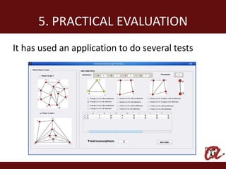
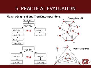
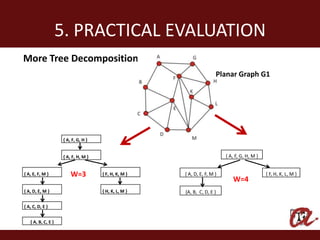
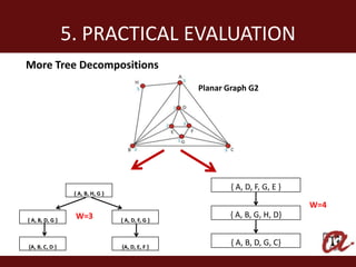
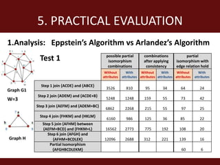
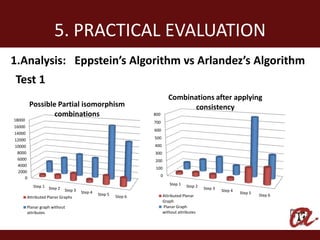
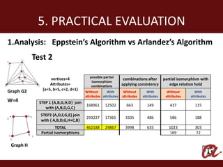
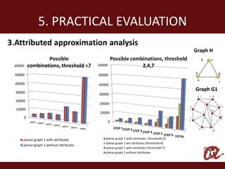


The document discusses various algorithms for matching planar graphs, focusing on both attributed and non-attributed graphs. It introduces Eppstein's algorithm and a new algorithm by Arlandez, highlighting their applications in reducing the number of combinations through attributes and different methods of edge functions. The practical evaluation compares these algorithms, providing insights into their efficiency and the impact of attributes on the matching process.


![[분석] Img2Braille - 이미지 to 점자 번역기](https://cdn.slidesharecdn.com/ss_thumbnails/img2braille-180213115720-thumbnail.jpg?width=640&height=640&fit=bounds)