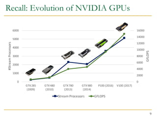
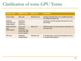
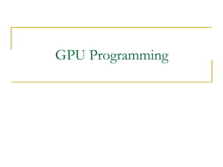
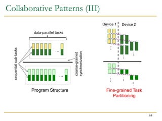
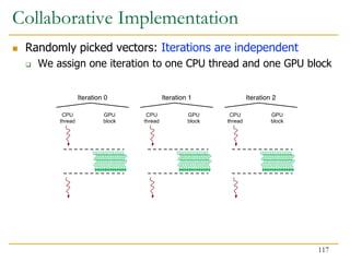
The document discusses GPU programming, highlighting key topics such as GPU architecture, memory management, programming models (like CUDA and OpenCL), and performance considerations including memory access and occupancy. It emphasizes the evolution of NVIDIA GPUs, the importance of coalesced memory access for performance, and the need for specialized algorithms to fully leverage GPU capabilities. Additionally, the lecture explores the benefits and challenges of utilizing GPUs for massively parallel processing tasks.

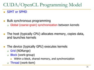
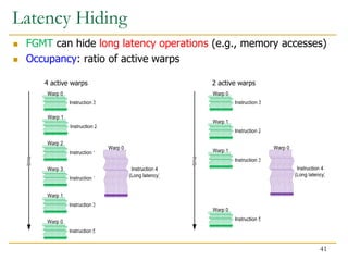
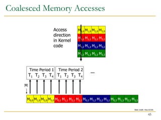
![Recall: Warp Execution
15
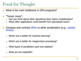
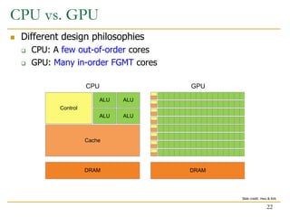
32-thread warp executing ADD A[tid],B[tid] C[tid]
C[1]
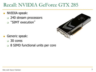
C[2]
C[0]
A[3] B[3]
A[4] B[4]
A[5] B[5]
A[6] B[6]
Execution using
one pipelined
functional unit
C[4]
C[8]
C[0]
A[12] B[12]
A[16] B[16]
A[20] B[20]
A[24] B[24]
C[5]
C[9]
C[1]
A[13] B[13]
A[17] B[17]
A[21] B[21]
A[25] B[25]
C[6]
C[10]
C[2]
A[14] B[14]
A[18] B[18]
A[22] B[22]
A[26] B[26]
C[7]
C[11]
C[3]
A[15] B[15]
A[19] B[19]
A[23] B[23]
A[27] B[27]
Execution using
four pipelined
functional units
Slide credit: Krste Asanovic
Time
Space
Time](https://image.slidesharecdn.com/comparch-fall2019-lecture17-gpuprogramming-afterlecture-240426190002-c85c3769/85/gpuprogram_lecture-architecture_designsn-15-320.jpg)
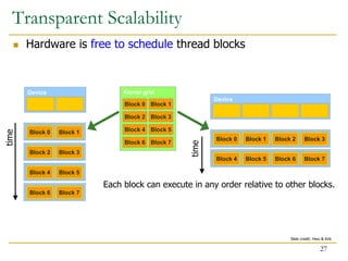
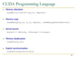
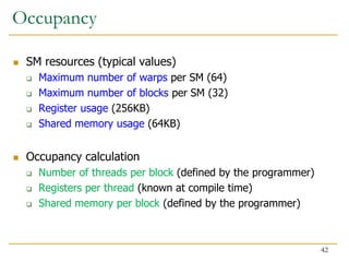
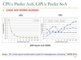
![Indexing and Memory Access
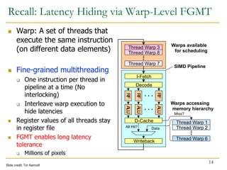
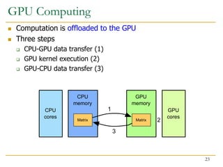
Images are 2D data structures
height x width
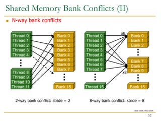
Image[j][i], where 0 ≤ j < height, and 0 ≤ i < width
Image[0][1]
Image[1][2]
31
0 1 2 3 4 5 6 7
0
1
2
3
4
5
6
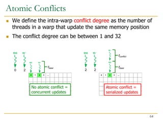
7](https://image.slidesharecdn.com/comparch-fall2019-lecture17-gpuprogramming-afterlecture-240426190002-c85c3769/85/gpuprogram_lecture-architecture_designsn-31-320.jpg)
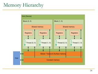
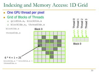
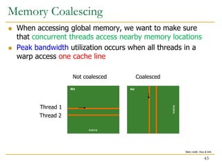
![Image Layout in Memory
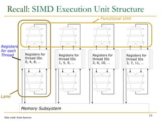
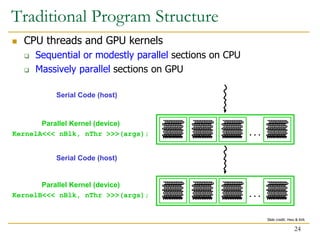
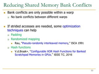
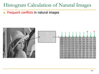
Row-major layout
Image[j][i] = Image[j x width + i]
Image[0][1] = Image[0 x 8 + 1]
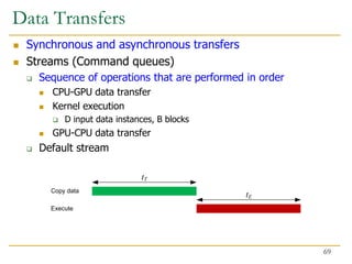
Image[1][2] = Image[1 x 8 + 2]
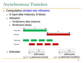
32
Stride = width](https://image.slidesharecdn.com/comparch-fall2019-lecture17-gpuprogramming-afterlecture-240426190002-c85c3769/85/gpuprogram_lecture-architecture_designsn-32-320.jpg)
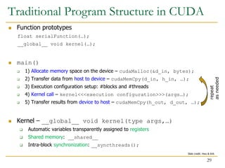
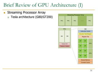
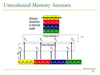
![Indexing and Memory Access: 2D Grid
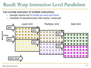
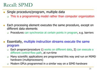
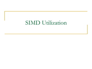
2D blocks
gridDim.x, gridDim.y
Block (0, 0)
blockIdx.x = 2
blockIdx.y = 1
Row = blockIdx.y *
blockDim.y + threadIdx.y
Row = 1 * 2 + 1 = 3
threadIdx.x = 1
threadIdx.y = 0
Col = blockIdx.x *
blockDim.x + threadIdx.x
Col = 0 * 2 + 1 = 1
Image[3][1] = Image[3 * 8 + 1]
34](https://image.slidesharecdn.com/comparch-fall2019-lecture17-gpuprogramming-afterlecture-240426190002-c85c3769/85/gpuprogram_lecture-architecture_designsn-34-320.jpg)
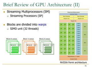
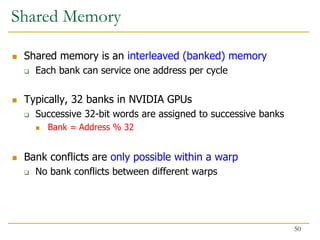
![AoS vs. SoA
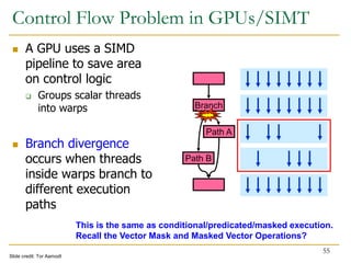
Array of Structures vs. Structure of Arrays
Tenemos 2 data layouts principales (AoS y SoA) y uno nuevo propuesto (A
ASTA permite transformar uno en otro más rápidamente y facilita hacerlo in-place
ahorrar memoria. En la siguiente figura se ven los tres:
Data Layout Alternatives
Array of
Structures
(AoS)
Array of
Structure of
Tiled Array
(ASTA)
struct foo{
float a;
float b;
float c;
int d;
} A[8];
struct foo{
float a[4];
float b[4];
float c[4];
int d[4];
} A[2];
Structure of
Arrays
(SoA)
struct foo{
float a[8];
float b[8];
float c[8];
int d[8];
} A;
Layout Conversion and Transposition 46](https://image.slidesharecdn.com/comparch-fall2019-lecture17-gpuprogramming-afterlecture-240426190002-c85c3769/85/gpuprogram_lecture-architecture_designsn-46-320.jpg)
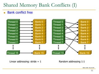
![Data Reuse
Same memory locations accessed by neighboring threads
for (int i = 0; i < 3; i++){
for (int j = 0; j < 3; j++){
sum += gauss[i][j] * Image[(i+row-1)*width + (j+col-1)];
}
}
48](https://image.slidesharecdn.com/comparch-fall2019-lecture17-gpuprogramming-afterlecture-240426190002-c85c3769/85/gpuprogram_lecture-architecture_designsn-48-320.jpg)
![Data Reuse: Tiling
To take advantage of data reuse, we divide the input into tiles
that can be loaded into shared memory
__shared__ int l_data[(L_SIZE+2)*(L_SIZE+2)];
…
Load tile into shared memory
__syncthreads();
for (int i = 0; i < 3; i++){
for (int j = 0; j < 3; j++){
sum += gauss[i][j] * l_data[(i+l_row-1)*(L_SIZE+2)+j+l_col-1];
}
}
49](https://image.slidesharecdn.com/comparch-fall2019-lecture17-gpuprogramming-afterlecture-240426190002-c85c3769/85/gpuprogram_lecture-architecture_designsn-49-320.jpg)
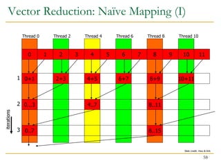
![Vector Reduction: Naïve Mapping (II)
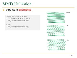
Program with low SIMD utilization
__shared__ float partialSum[]
unsigned int t = threadIdx.x;
for (int stride = 1; stride < blockDim.x; stride *= 2) {
__syncthreads();
if (t % (2*stride) == 0)
partialSum[t] += partialSum[t + stride];
}
59](https://image.slidesharecdn.com/comparch-fall2019-lecture17-gpuprogramming-afterlecture-240426190002-c85c3769/85/gpuprogram_lecture-architecture_designsn-59-320.jpg)
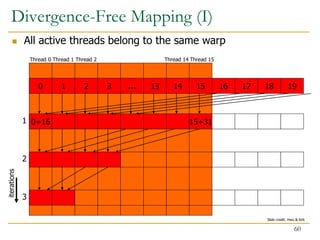
![Divergence-Free Mapping (II)
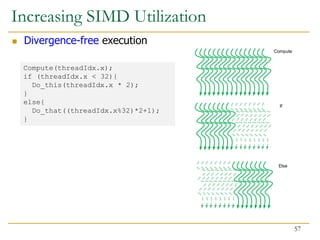
Program with high SIMD utilization
__shared__ float partialSum[]
unsigned int t = threadIdx.x;
for (int stride = blockDim.x; stride > 1; stride >> 1){
__syncthreads();
if (t < stride)
partialSum[t] += partialSum[t + stride];
}
61](https://image.slidesharecdn.com/comparch-fall2019-lecture17-gpuprogramming-afterlecture-240426190002-c85c3769/85/gpuprogram_lecture-architecture_designsn-61-320.jpg)
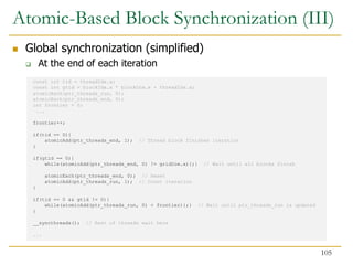
![ Atomic Operations are needed when threads might update the
same memory locations at the same time
CUDA: int atomicAdd(int*, int);
PTX: atom.shared.add.u32 %r25, [%rd14], %r24;
SASS:
/*00a0*/ LDSLK P0, R9, [R8];
/*00a8*/ @P0 IADD R10, R9, R7;
/*00b0*/ @P0 STSCUL P1, [R8], R10;
/*00b8*/ @!P1 BRA 0xa0;
/*01f8*/ ATOMS.ADD RZ, [R7], R11;
Native atomic operations for
32-bit integer, and 32-bit and
64-bit atomicCAS
Tesla, Fermi, Kepler Maxwell, Pascal, Volta
Shared Memory Atomic Operations
63](https://image.slidesharecdn.com/comparch-fall2019-lecture17-gpuprogramming-afterlecture-240426190002-c85c3769/85/gpuprogram_lecture-architecture_designsn-63-320.jpg)
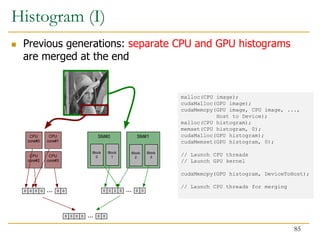
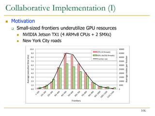
![Histogram Calculation
Histograms count the number of data instances in disjoint
categories (bins)
for (each pixel i in image I){
Pixel = I[i] // Read pixel
Pixel’ = Computation(Pixel) // Optional computation
Histogram[Pixel’]++ // Vote in histogram bin
}
Atomic additions
65](https://image.slidesharecdn.com/comparch-fall2019-lecture17-gpuprogramming-afterlecture-240426190002-c85c3769/85/gpuprogram_lecture-architecture_designsn-65-320.jpg)
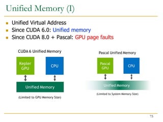
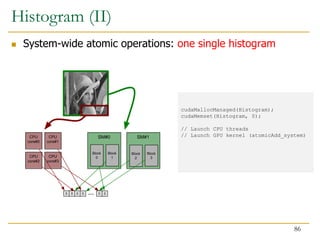
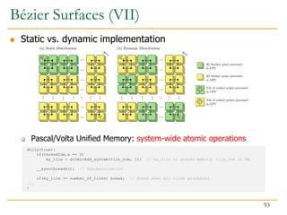
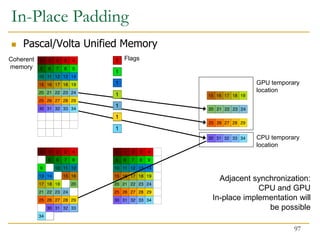
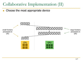
![ Fine-grain heterogeneity becomes possible with
Pascal/Volta architecture
Pascal/Volta Unified Memory
CPU-GPU memory coherence
System-wide atomic operations
// Allocate input
cudaMallocManaged(input, ...);
// Allocate output
cudaMallocManaged(output, ...);
// Launch GPU kernel
gpu_kernel<<<blocks, threads>>> (output, input, ...);
// CPU can do things here
output[x] = input[y];
output[x+1].fetch_add(1);
Fine-Grained Heterogeneity
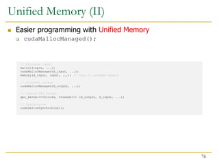
78](https://image.slidesharecdn.com/comparch-fall2019-lecture17-gpuprogramming-afterlecture-240426190002-c85c3769/85/gpuprogram_lecture-architecture_designsn-78-320.jpg)
![Since CUDA 8.0
Unified memory
cudaMallocManaged(&h_in, in_size);
System-wide atomics
old = atomicAdd_system(&h_out[x], inc);
79](https://image.slidesharecdn.com/comparch-fall2019-lecture17-gpuprogramming-afterlecture-240426190002-c85c3769/85/gpuprogram_lecture-architecture_designsn-79-320.jpg)
![Since OpenCL 2.0
Shared virtual memory
XYZ * h_in = (XYZ *)clSVMAlloc(
ocl.clContext, CL_MEM_SVM_FINE_GRAIN_BUFFER, in_size, 0);
More flags:
CL_MEM_READ_WRITE
CL_MEM_SVM_ATOMICS
C++11 atomic operations
(memory_scope_all_svm_devices)
old = atomic_fetch_add(&h_out[x], inc);
80](https://image.slidesharecdn.com/comparch-fall2019-lecture17-gpuprogramming-afterlecture-240426190002-c85c3769/85/gpuprogram_lecture-architecture_designsn-80-320.jpg)
![C++AMP (HCC)
Unified memory space (HSA)
XYZ *h_in = (XYZ *)malloc(in_size);
C++11 atomic operations
(memory_scope_all_svm_devices)
Platform atomics (HSA)
old = atomic_fetch_add(&h_out[x], inc);
81](https://image.slidesharecdn.com/comparch-fall2019-lecture17-gpuprogramming-afterlecture-240426190002-c85c3769/85/gpuprogram_lecture-architecture_designsn-81-320.jpg)
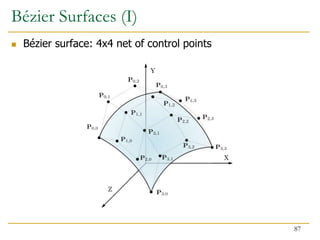
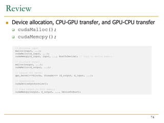
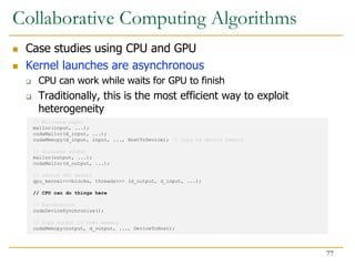
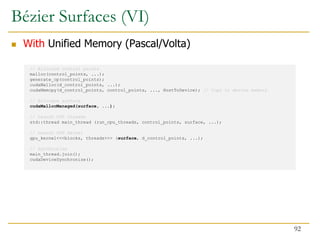
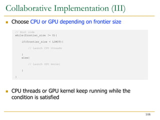
![// Allocate control points
malloc(control_points, ...);
generate_cp(control_points);
cudaMalloc(d_control_points, ...);
cudaMemcpy(d_control_points, control_points, ..., HostToDevice); // Copy to device memory
// Allocate surface
malloc(surface, ...);
cudaMalloc(d_surface, ...);
// Launch CPU threads
std::thread main_thread (run_cpu_threads, control_points, surface, ...);
// Launch GPU kernel
gpu_kernel<<<blocks, threads>>> (d_surface, d_control_points, ...);
// Synchronize
main_thread.join();
cudaDeviceSynchronize();
// Copy gpu part of surface to host memory
cudaMemcpy(&surface[end_of_cpu_part], d_surface, ..., DeviceToHost);
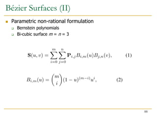
Bézier Surfaces (IV)
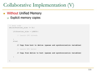
Without Unified Memory
90](https://image.slidesharecdn.com/comparch-fall2019-lecture17-gpuprogramming-afterlecture-240426190002-c85c3769/85/gpuprogram_lecture-architecture_designsn-90-320.jpg)
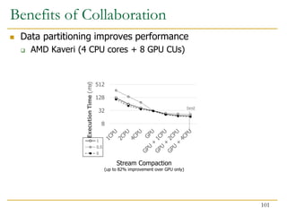
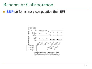
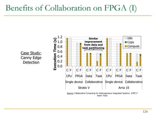
![Benefits of Collaboration on FPGA (III)
126
Sitao Huang, Li-Wen Chang, Izzat El Hajj, Simon Garcia De Gonzalo, Juan Gomez-Luna, Sai Rahul
Chalamalasetti, Mohamed El-Hadedy, Dejan Milojicic, Onur Mutlu, Deming Chen, and Wen-mei Hwu,
"Analysis and Modeling of Collaborative Execution Strategies for Heterogeneous CPU-
FPGA Architectures"
Proceedings of the 10th ACM/SPEC International Conference on Performance Engineering (ICPE),
Mumbai, India, April 2019.
[Slides (pptx) (pdf)]
[Chai CPU-FPGA Benchmark Suite]](https://image.slidesharecdn.com/comparch-fall2019-lecture17-gpuprogramming-afterlecture-240426190002-c85c3769/85/gpuprogram_lecture-architecture_designsn-126-320.jpg)