This document discusses clustering and density estimation techniques. It begins by introducing mixture models for density estimation, where the density is represented as a weighted sum of component densities. It then discusses k-means clustering, which groups data by finding cluster centers (prototypes) that minimize within-cluster variance. The document also covers Expectation-Maximization (EM) for parameter estimation in mixture models, hierarchical clustering approaches, and nonparametric density estimation methods like kernel density estimation and k-nearest neighbor estimation that make few assumptions about the underlying distributions.

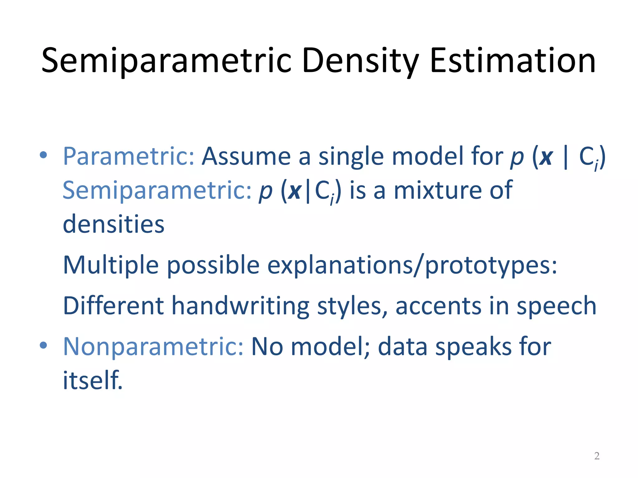
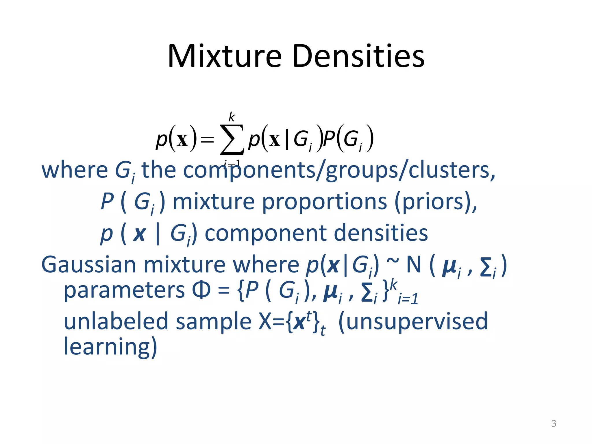
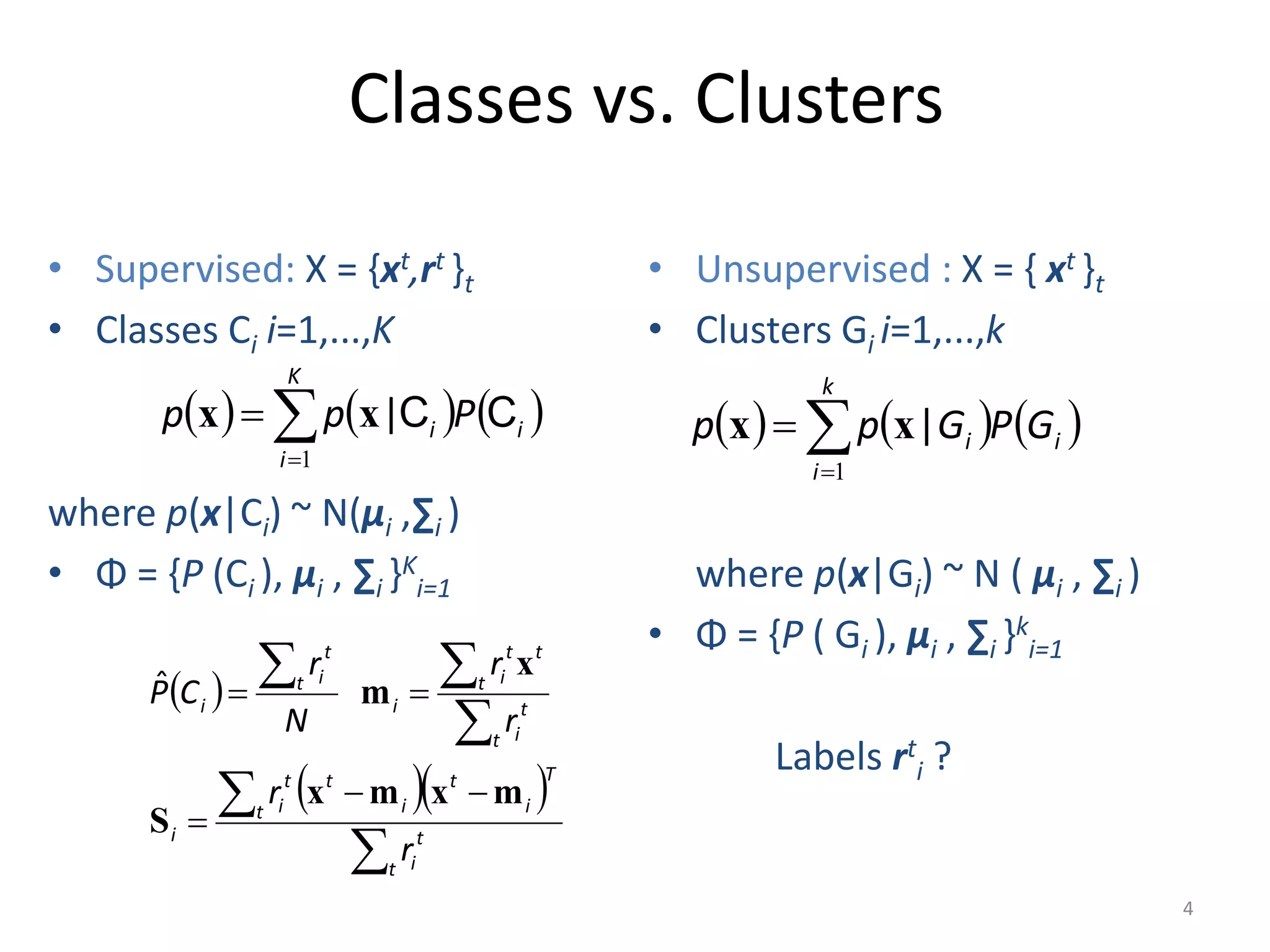
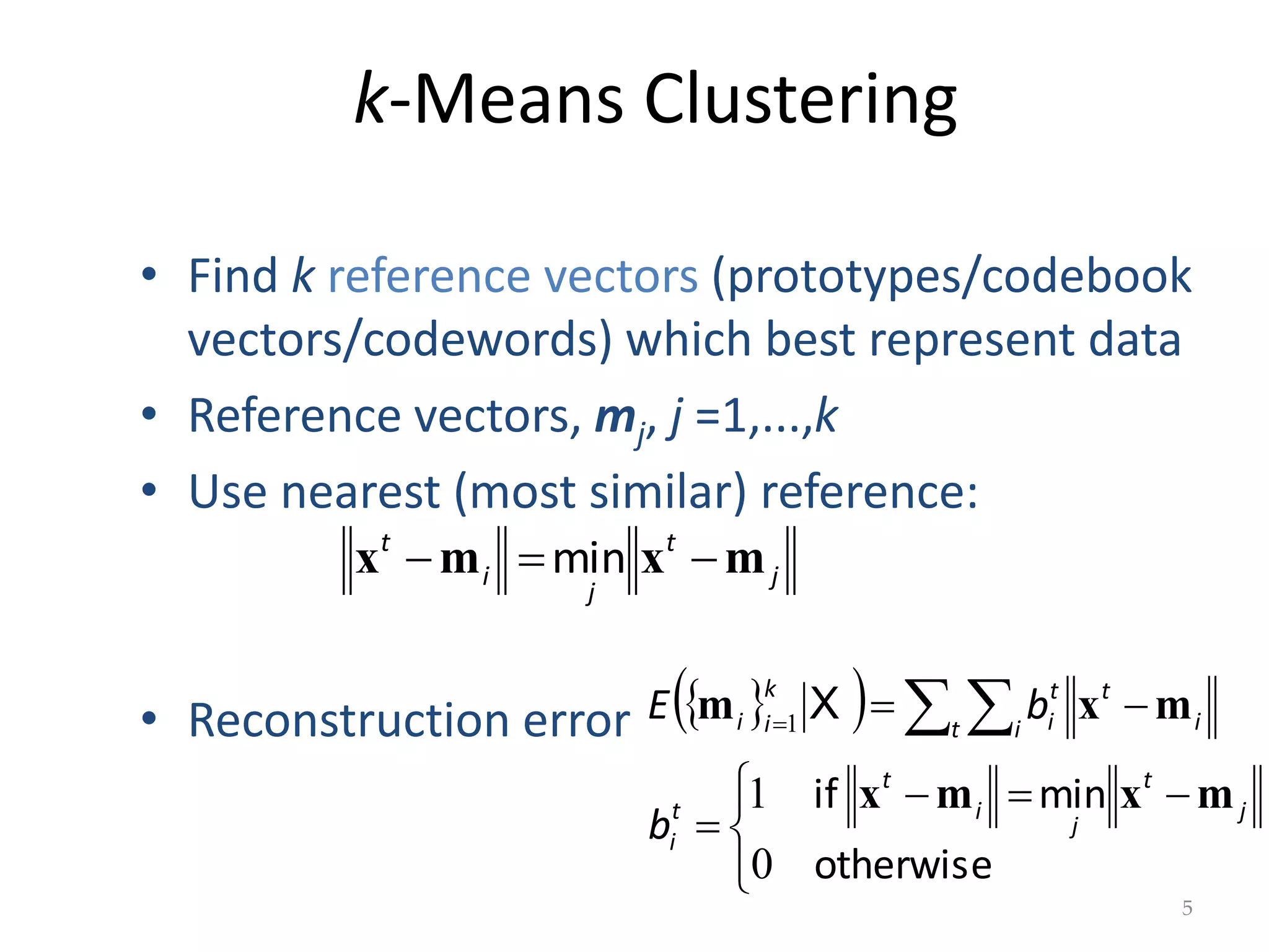
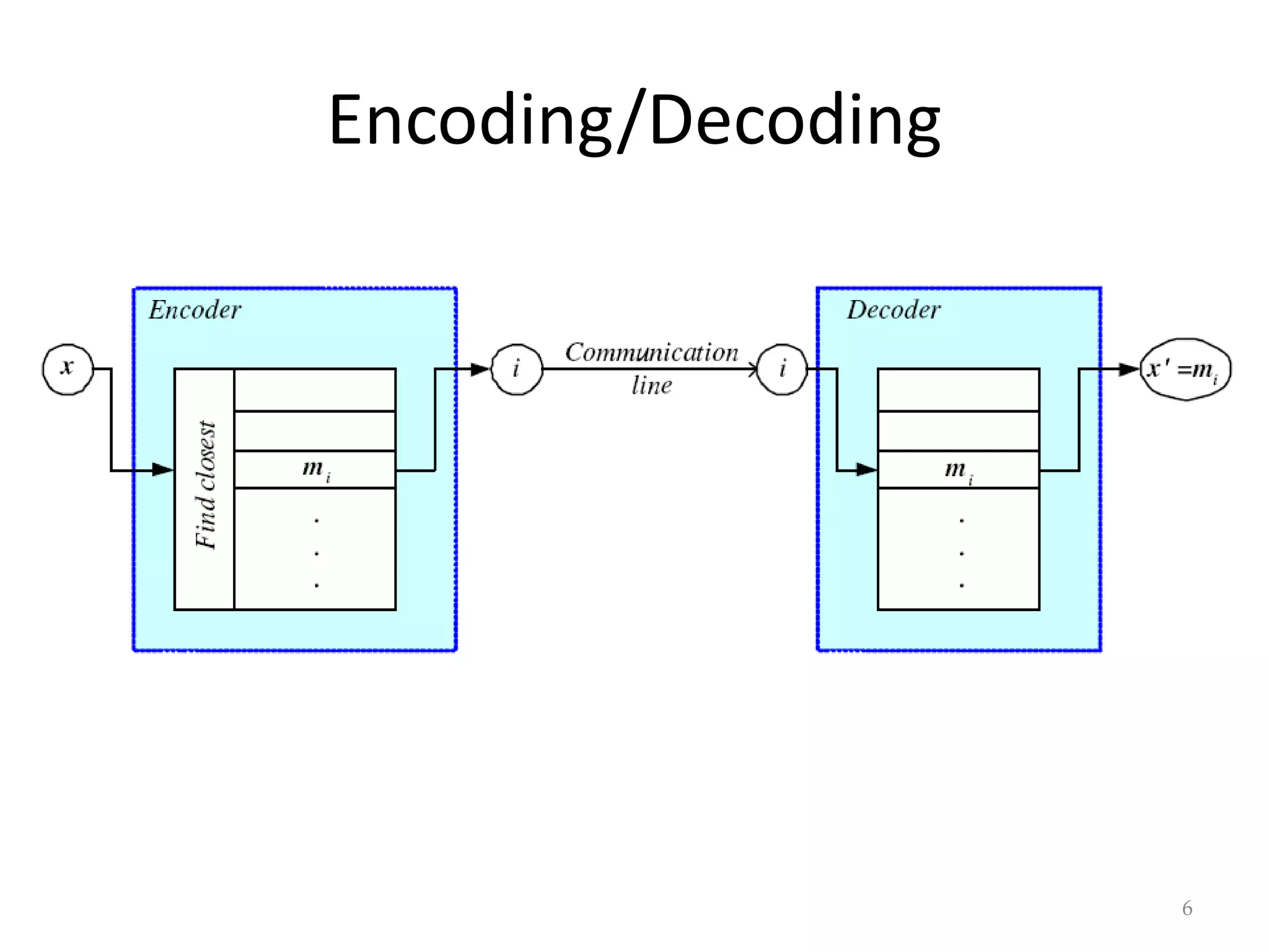
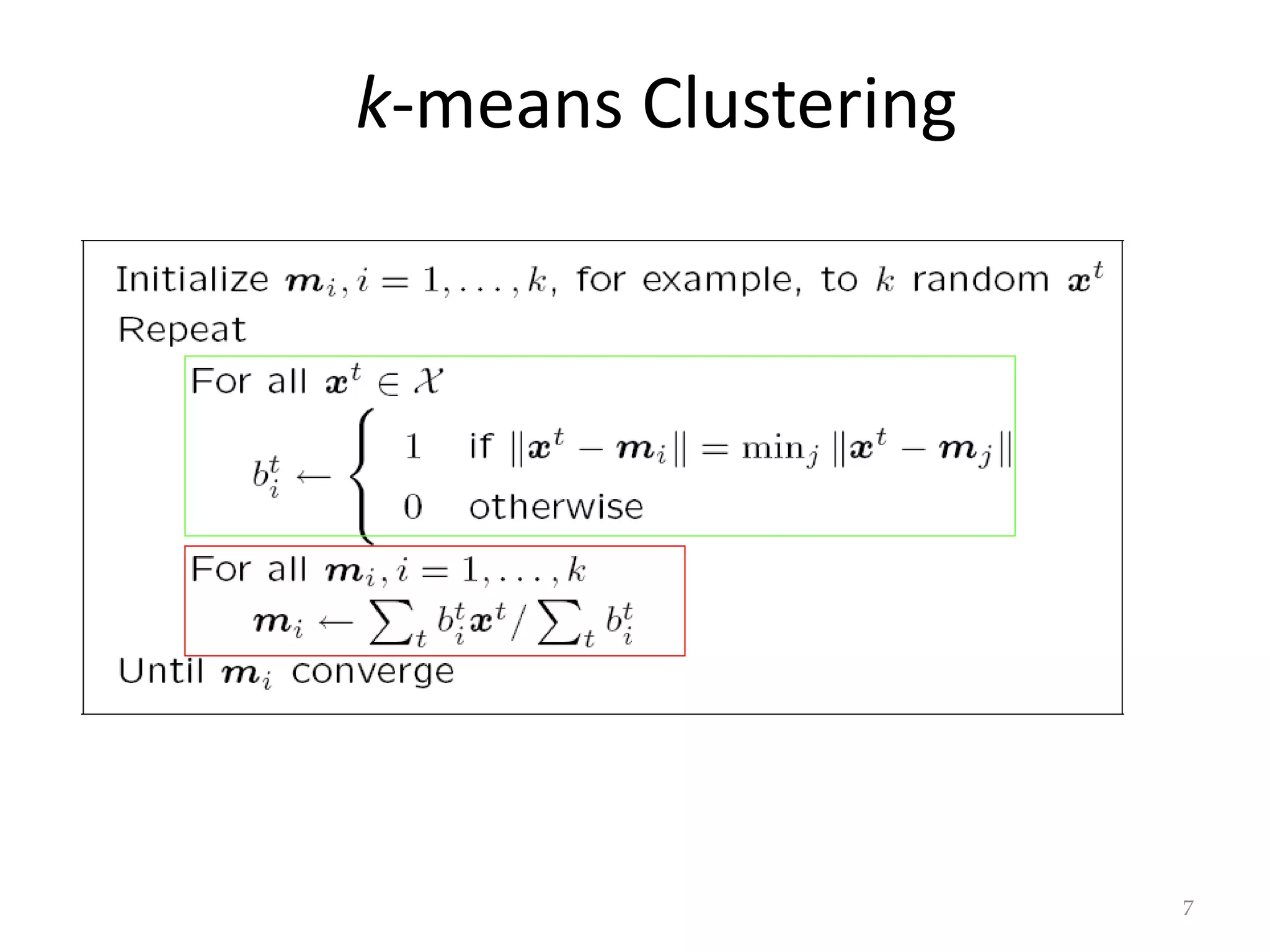
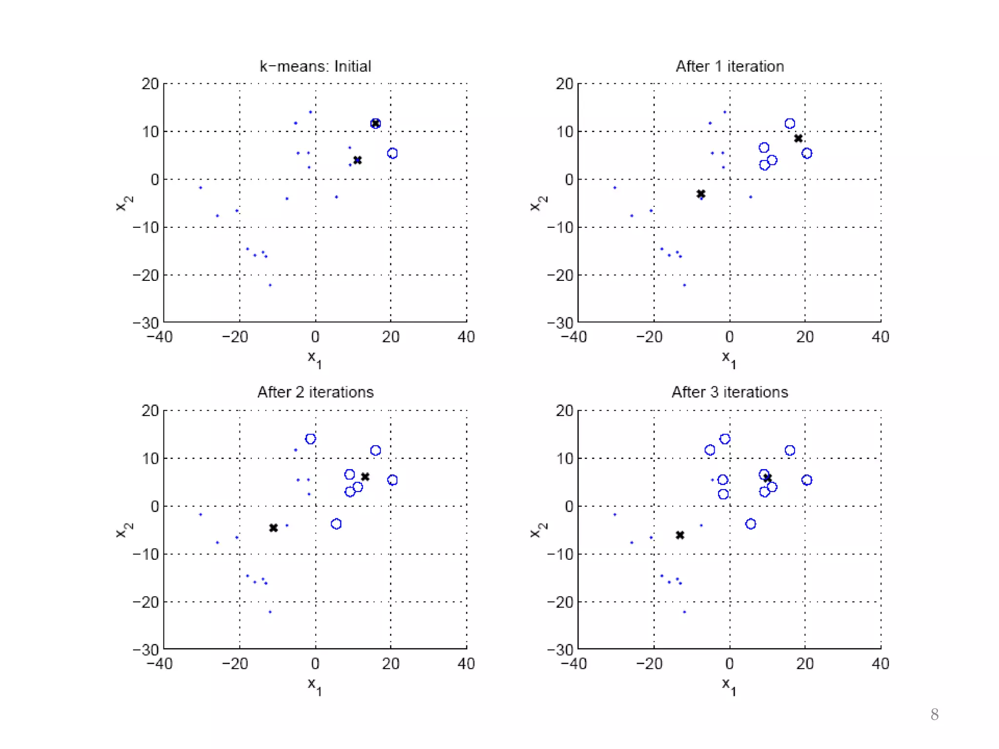
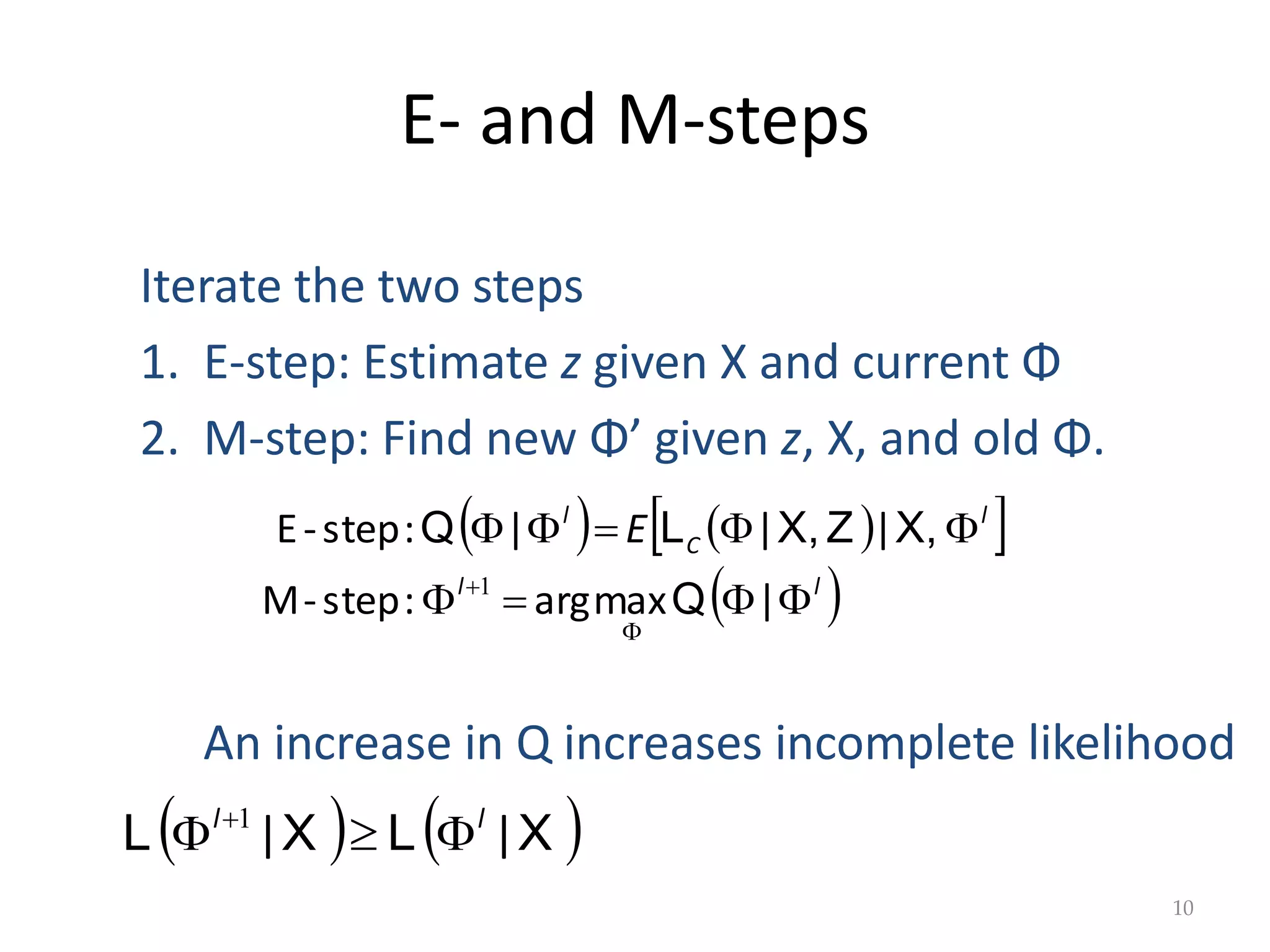
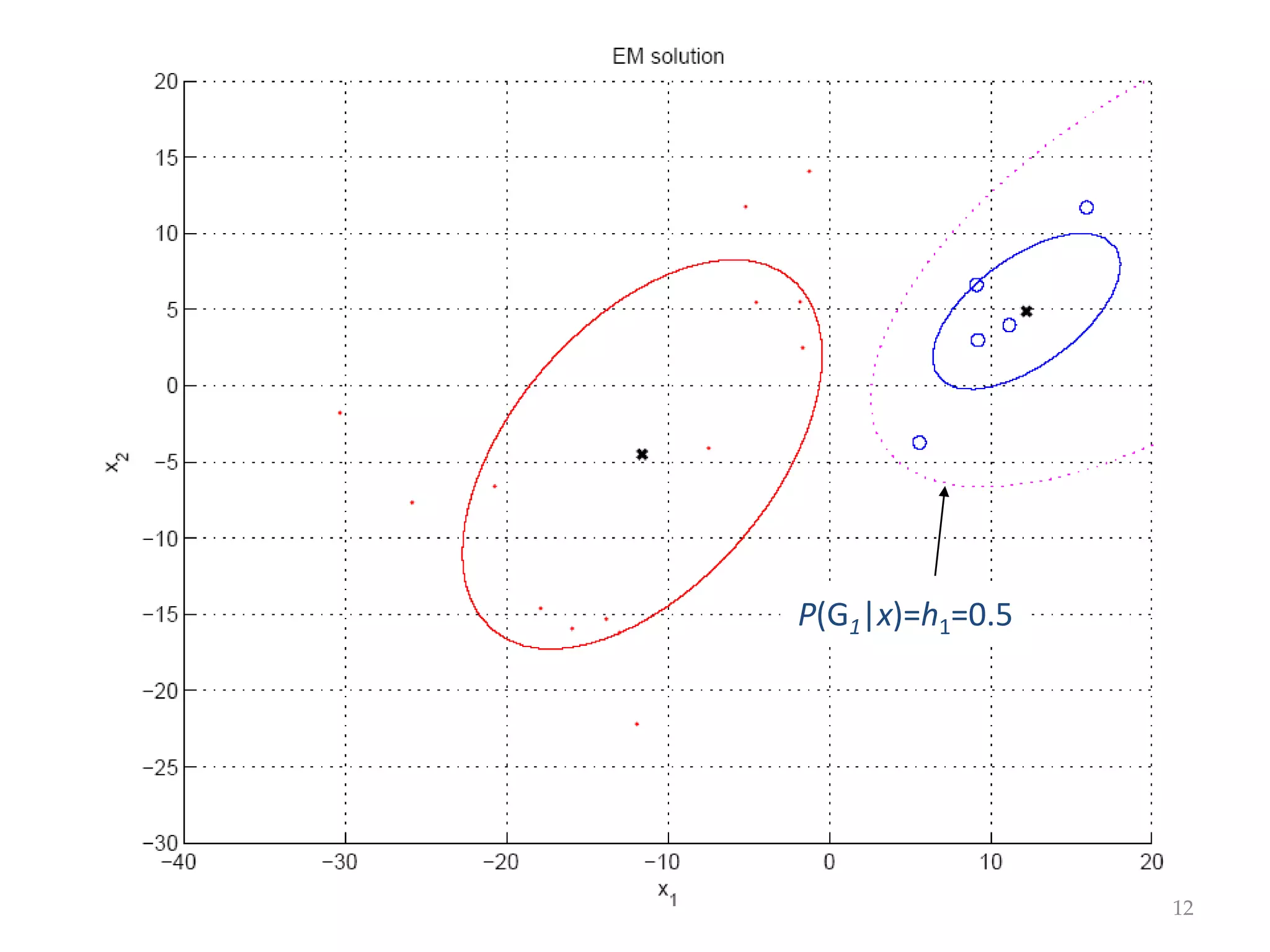
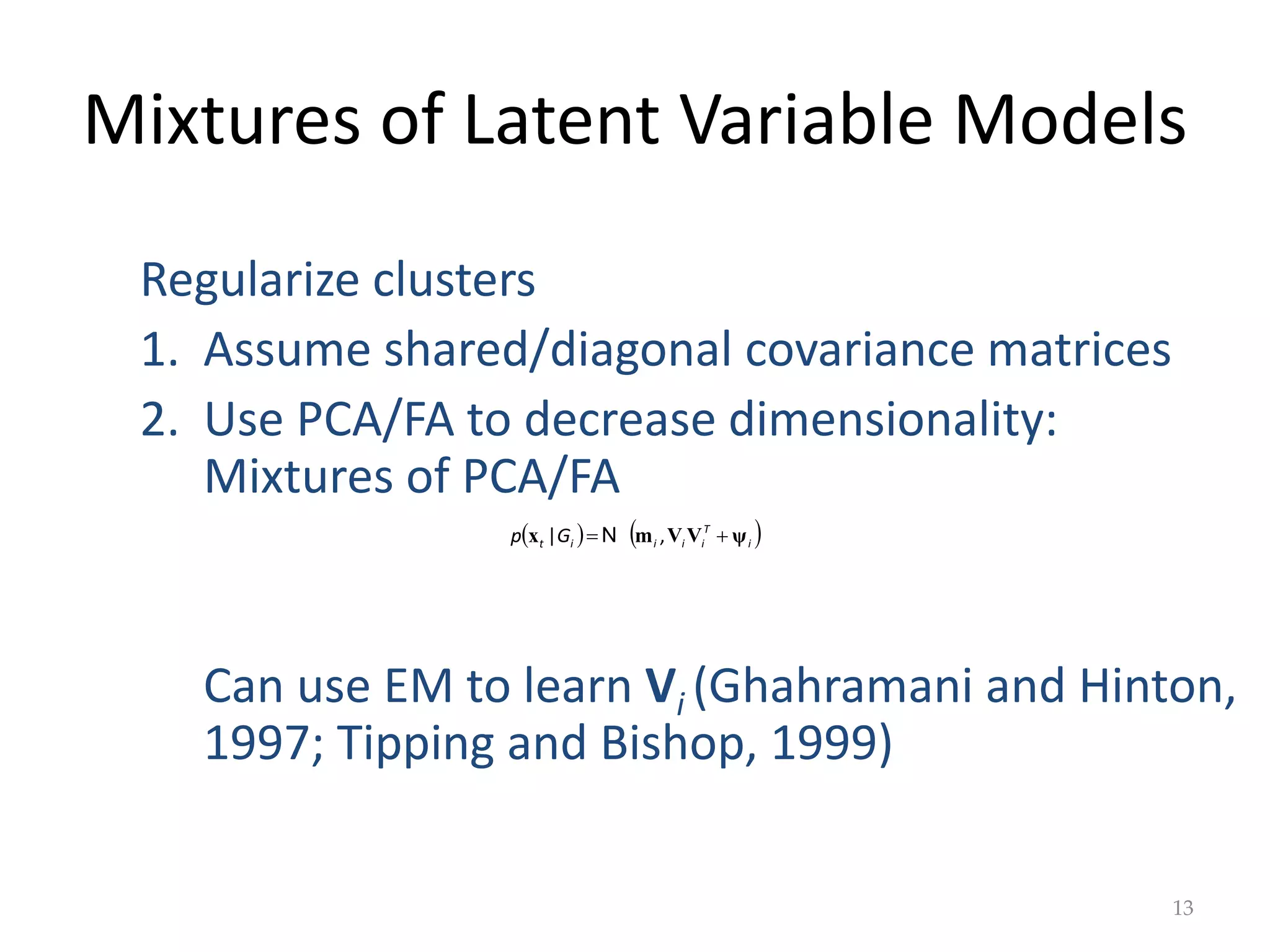
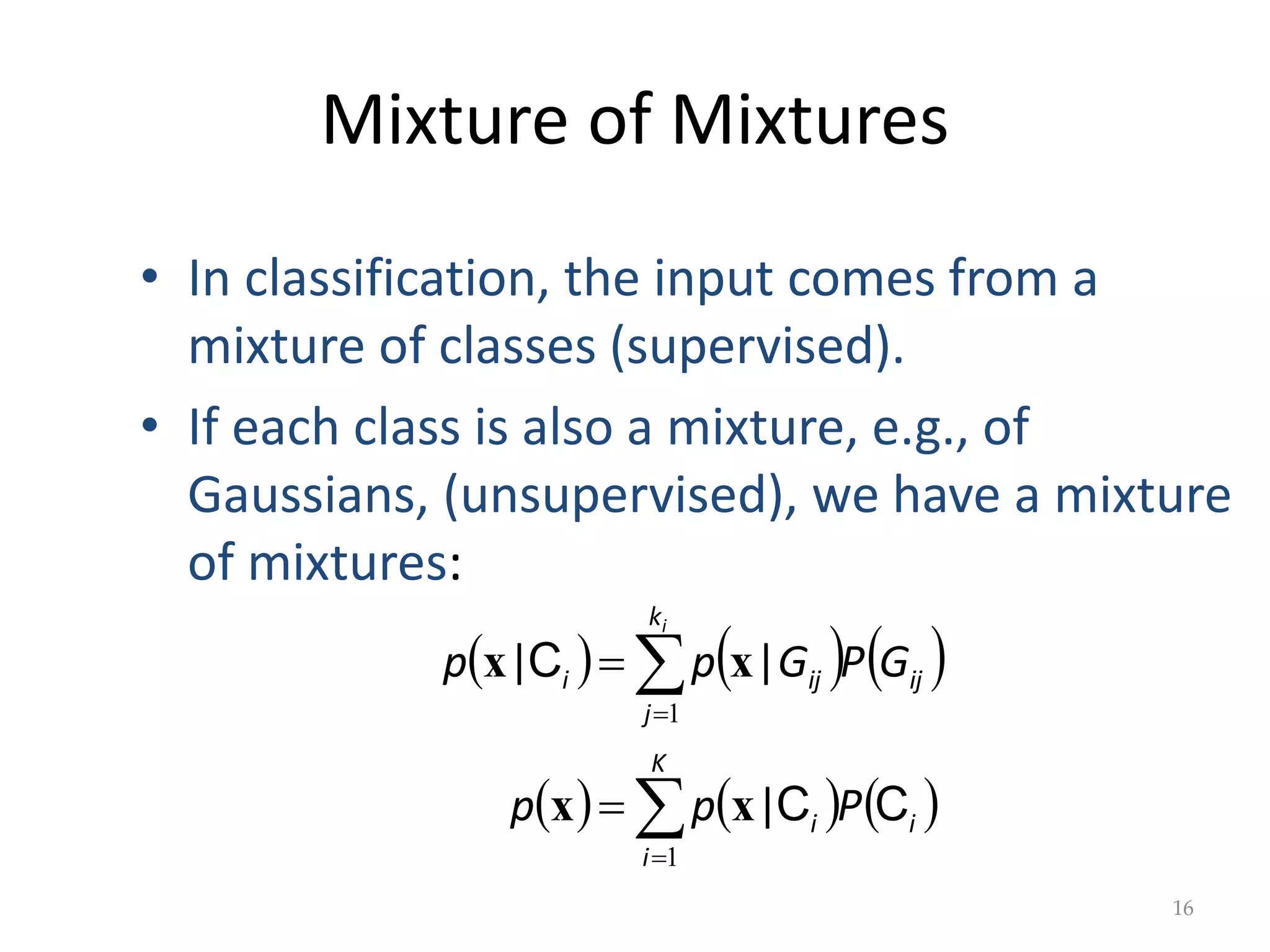
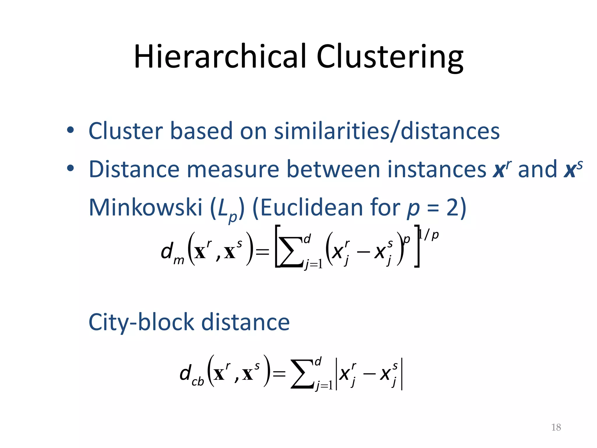
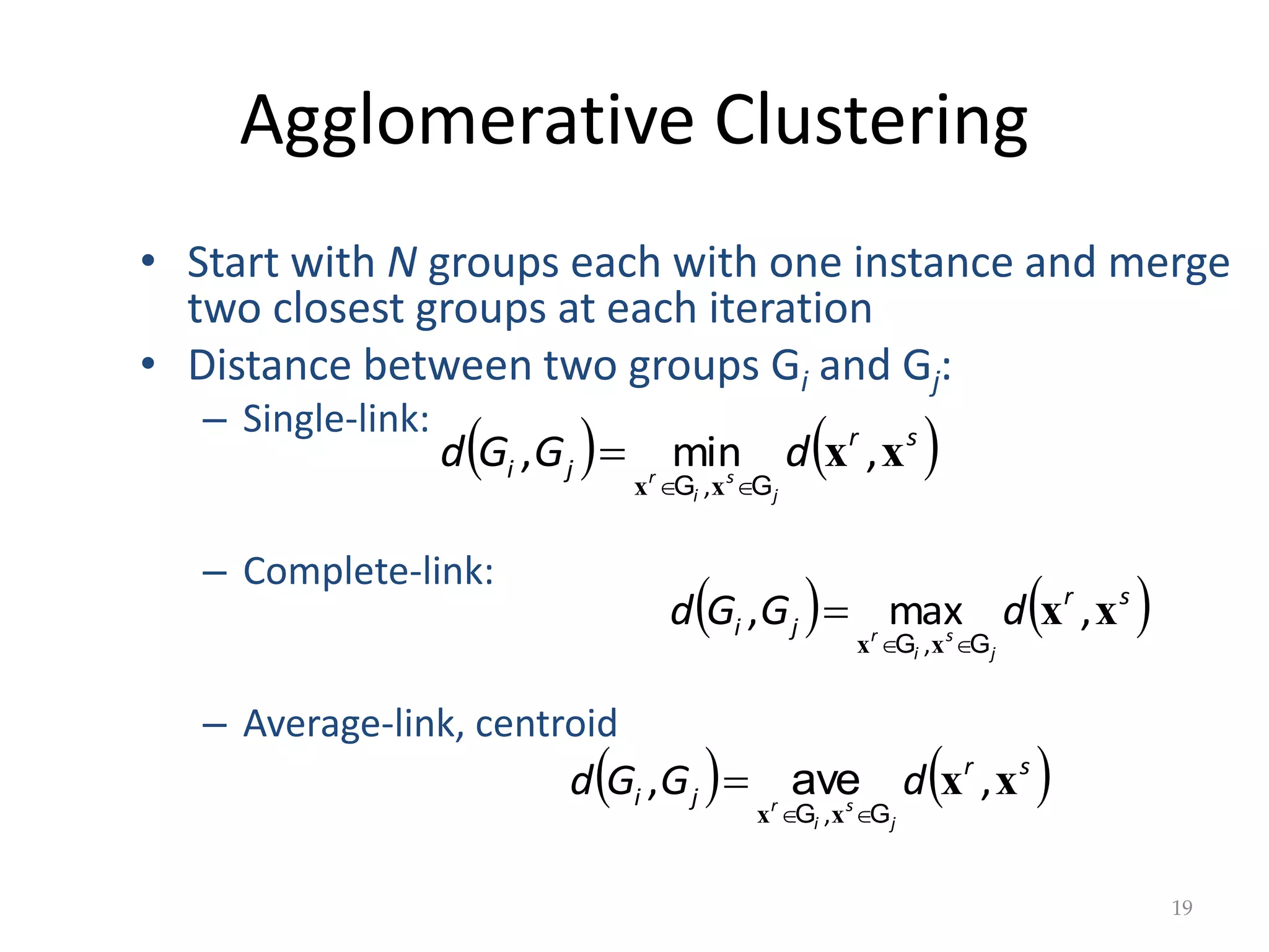
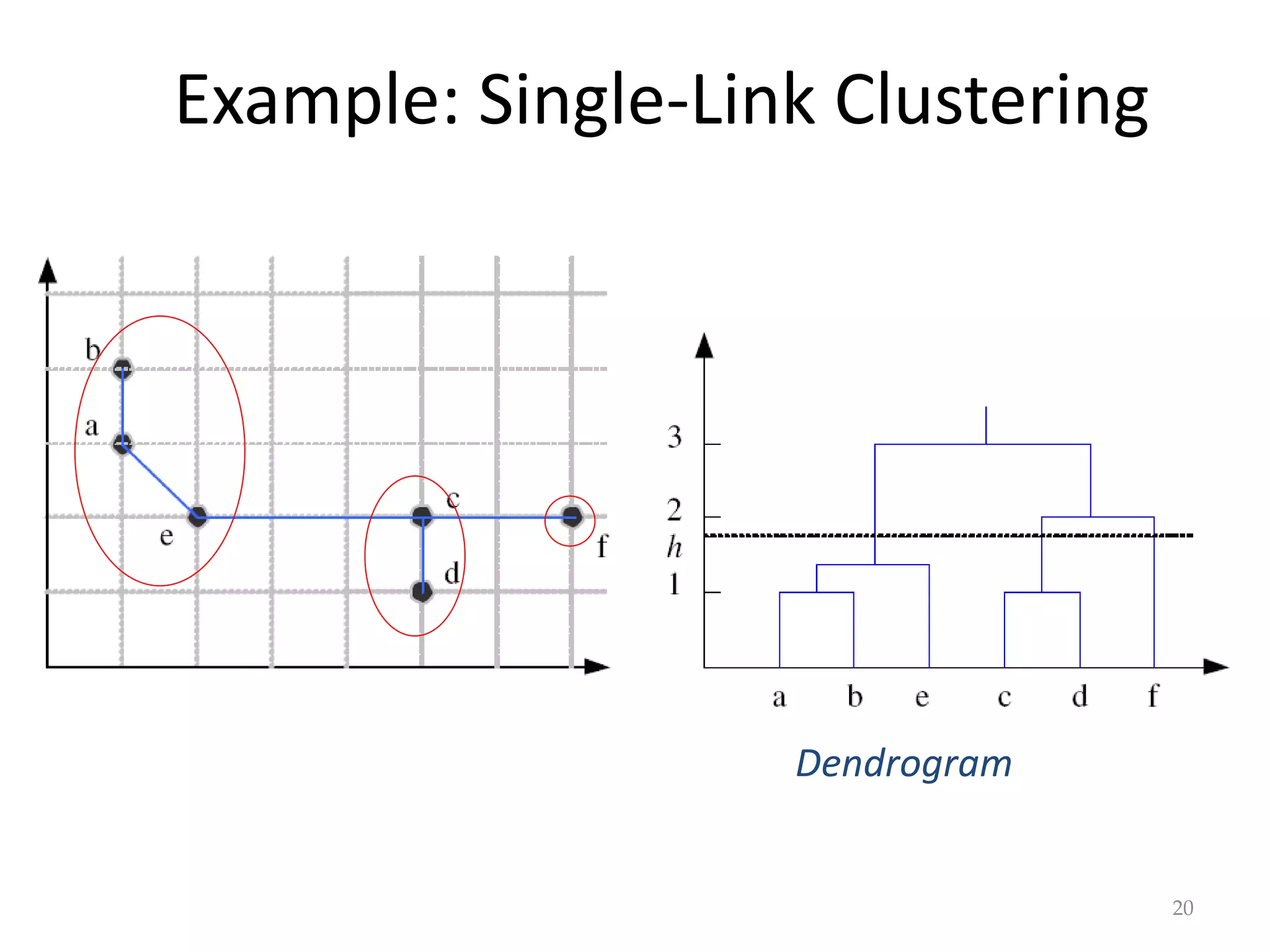
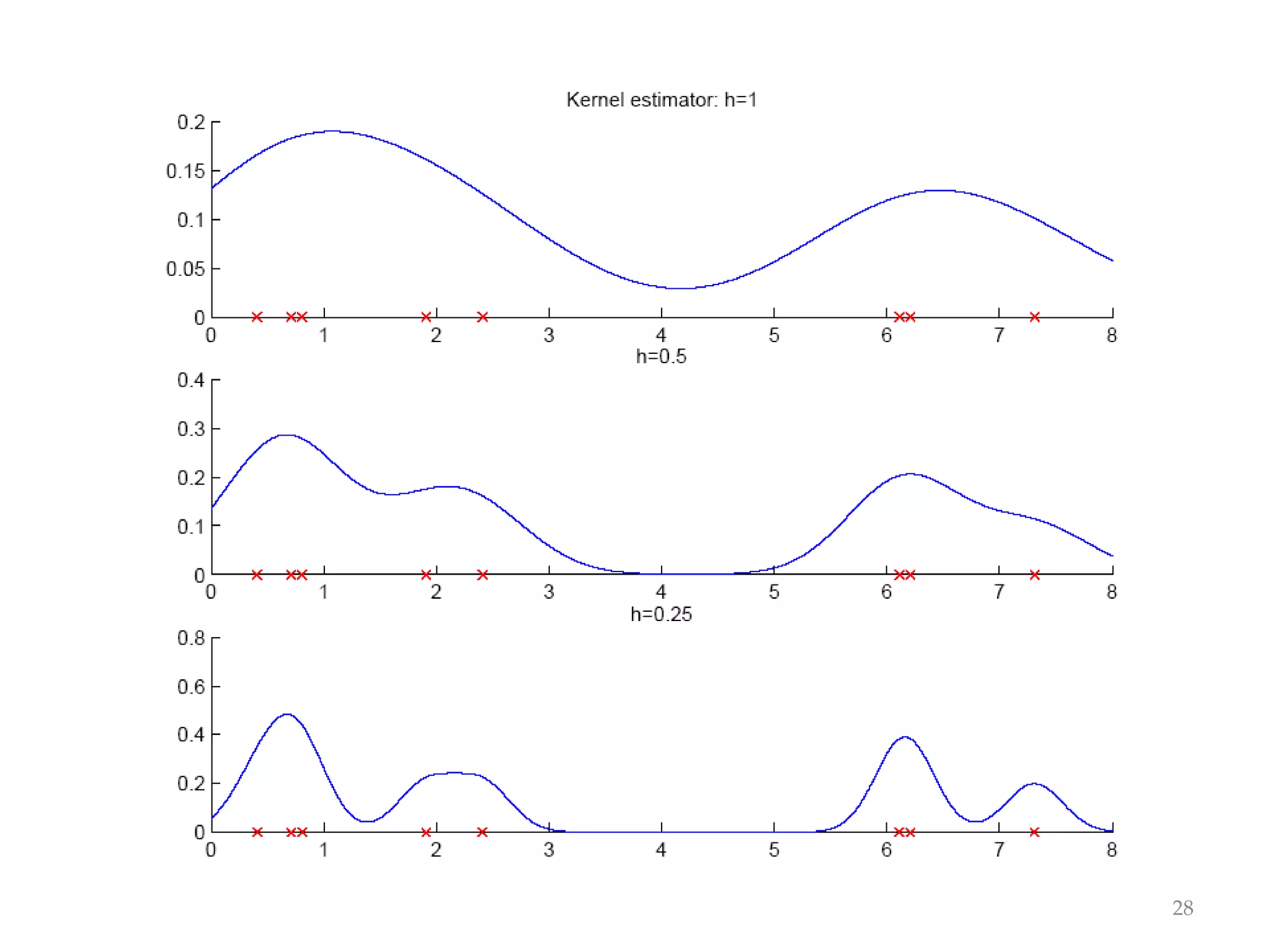
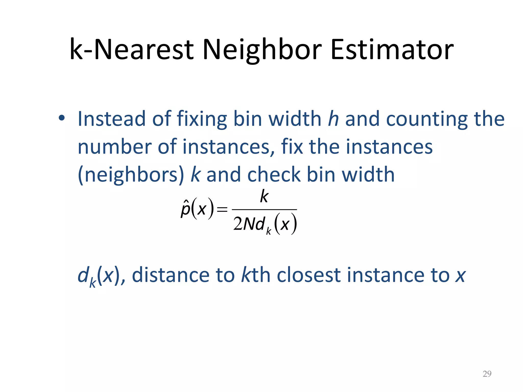
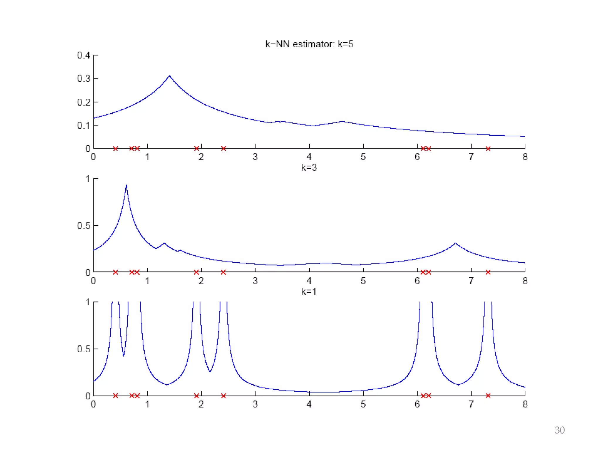
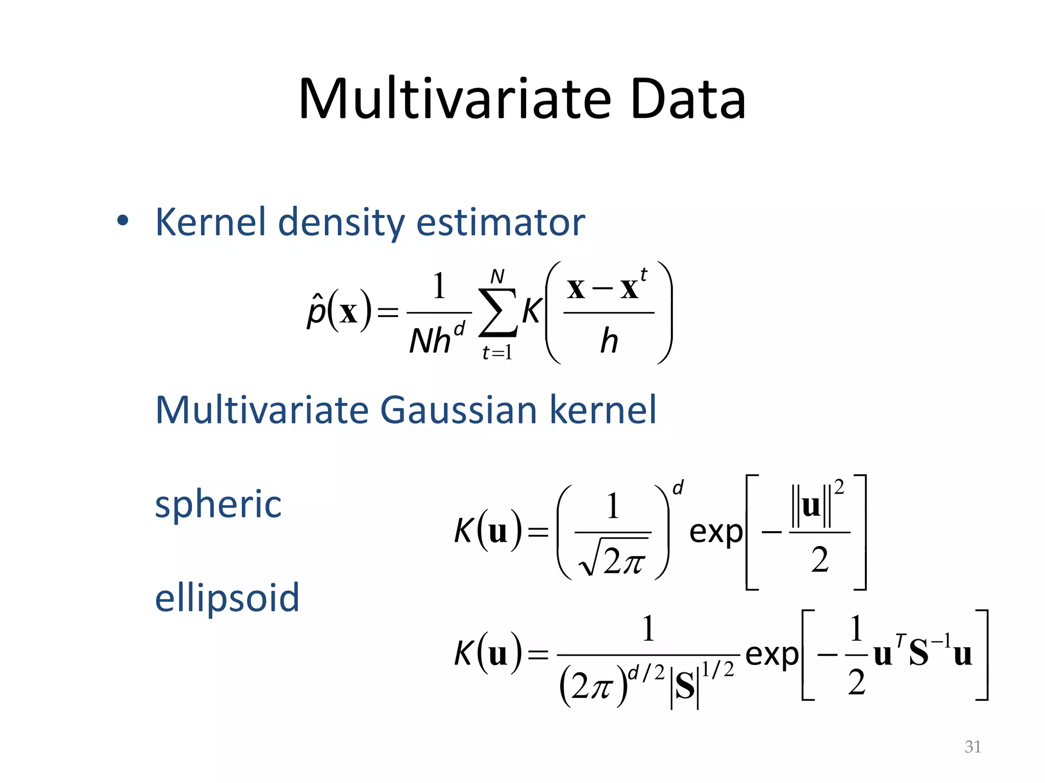
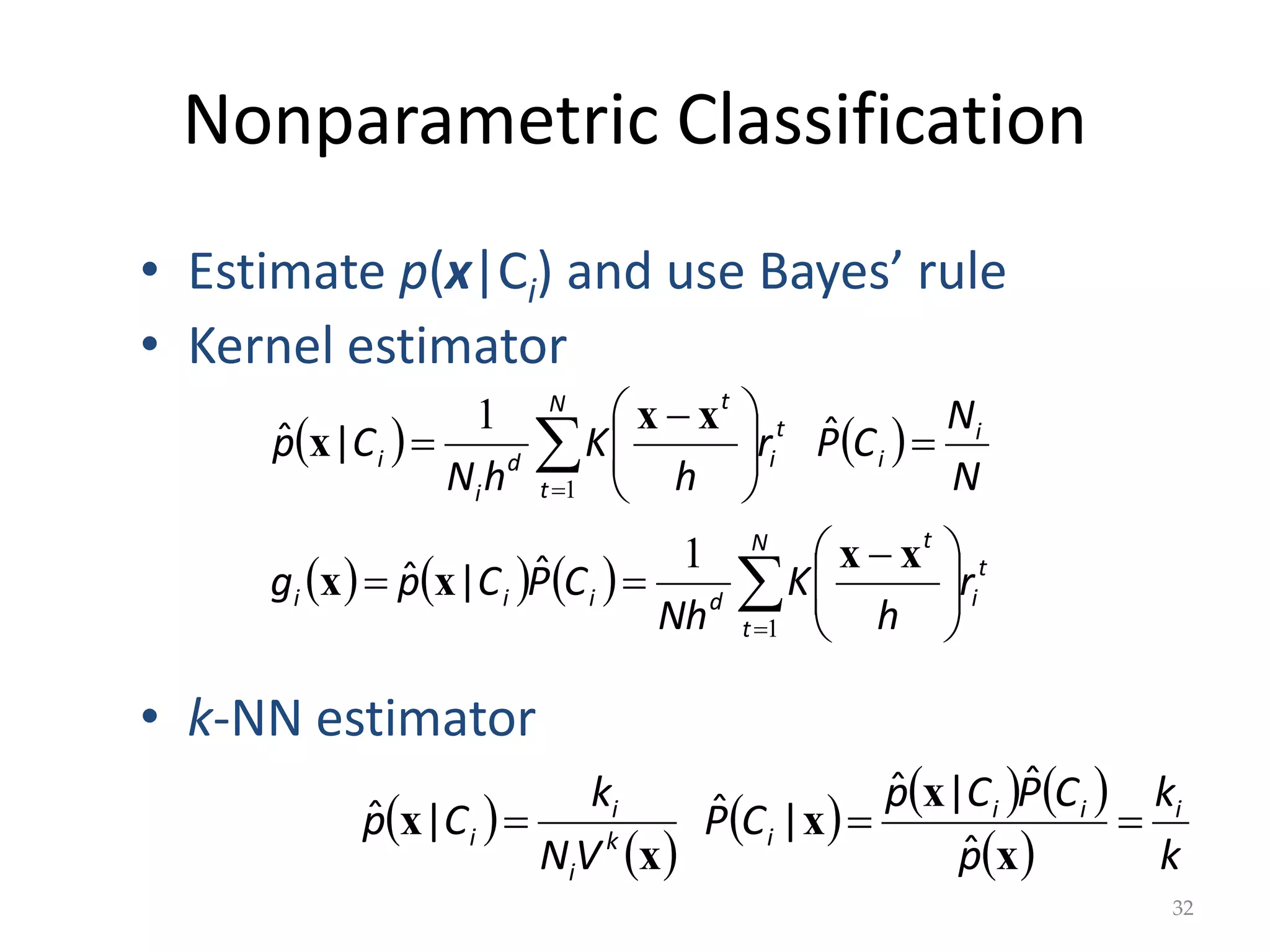
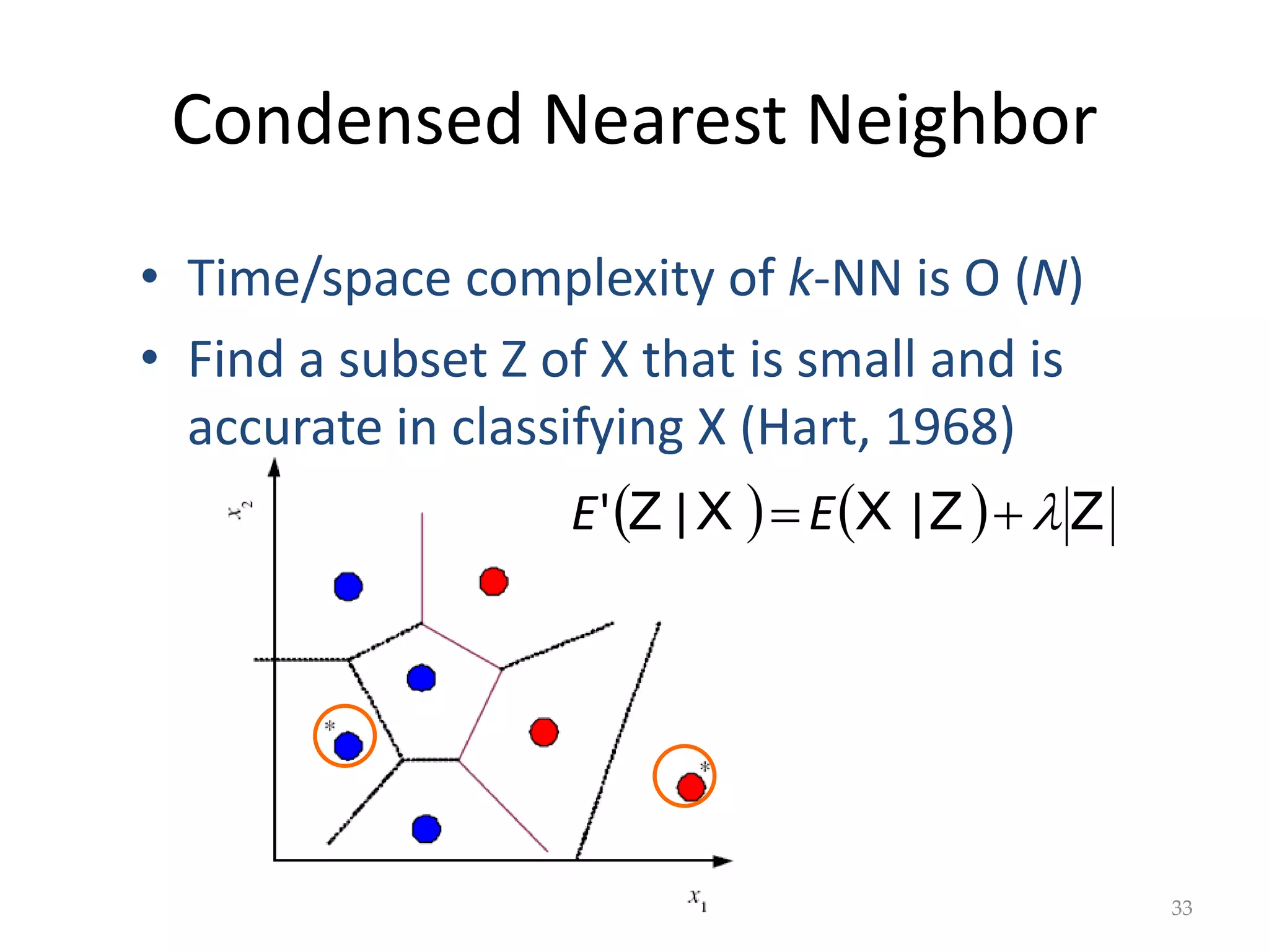
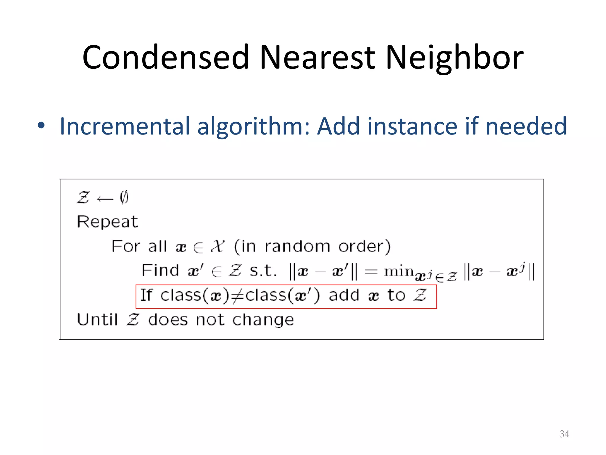
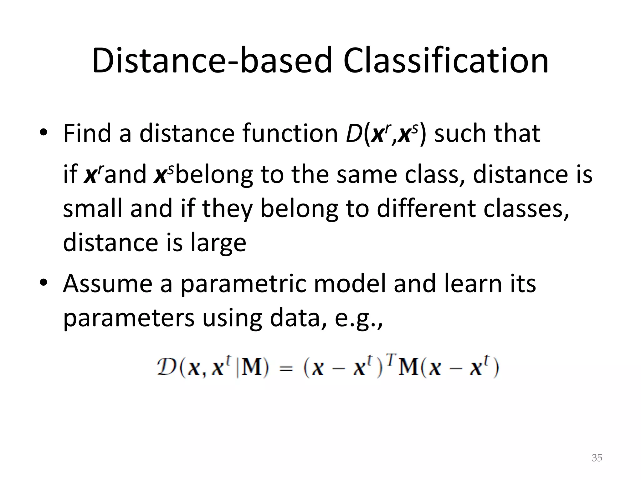
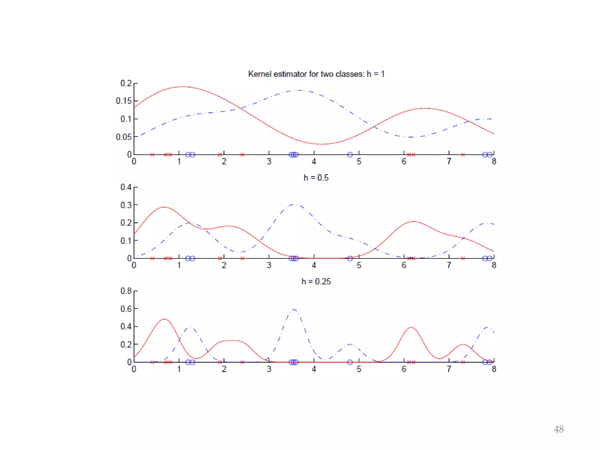
1. Unit-3:
Clustering

2. Semiparametric Density Estimation
• Parametric: Assume a single model for p (x | Ci)
Semiparametric: p (x|Ci) is a mixture of
densities
Multiple possible explanations/prototypes:
Different handwriting styles, accents in speech
• Nonparametric: No model; data speaks for
itself.
2

3. Mixture Densities
     



k
i
i
i G
P
G
p
p
1
|
x
x
3
where Gi the components/groups/clusters,
P ( Gi ) mixture proportions (priors),
p ( x | Gi) component densities
Gaussian mixture where p(x|Gi) ~ N ( μi , ∑i )
parameters Φ = {P ( Gi ), μi , ∑i }k
i=1
unlabeled sample X={xt}t (unsupervised
learning)

4. Classes vs. Clusters
• Supervised: X = {xt,rt }t
• Classes Ci i=1,...,K
where p(x|Ci) ~ N(μi ,∑i )
• Φ = {P (Ci ), μi , ∑i }K
i=1
• Unsupervised : X = { xt }t
• Clusters Gi i=1,...,k
where p(x|Gi) ~ N ( μi , ∑i )
• Φ = {P ( Gi ), μi , ∑i }k
i=1
Labels rt
i ?
4
     



k
i
i
i G
P
G
p
p
1
|
x
x
     



K
i
i
i P
p
p
1
C
C
|
x
x
 
  










t
t
i
T
i
t
t i
t
t
i
i
t
t
i
t
t
t
i
i
t
t
i
i
r
r
r
r
N
r
C
P
m
x
m
x
x
m
S
ˆ

5. k-Means Clustering
j
t
j
i
t
m
x
m
x 

 min
5
• Find k reference vectors (prototypes/codebook
vectors/codewords) which best represent data
• Reference vectors, mj, j =1,...,k
• Use nearest (most similar) reference:
• Reconstruction error  
 




 




  

otherwise
min
if
0
1
1
j
t
j
i
t
t
i
t i i
t
t
i
k
i
i
b
b
E
m
x
m
x
m
x
m X

6. Encoding/Decoding




 



otherwise
0
min
if
1 j
t
j
i
t
t
i
b
m
x
m
x
6

7. k-means Clustering
7

8. 8

9. Expectation-Maximization (EM)
   
   
 






t
k
i
i
i
t
t
t
G
P
G
p
p
1
|
log
|
log
|
x
x
X
L
9
• Log likelihood with a mixture model
• Assume hidden variables z, which when known, make
optimization much simpler
• Complete likelihood, Lc(Φ |X,Z), in terms of x and z
• Incomplete likelihood, L(Φ |X), in terms of x

10. E- and M-steps
   
 
 
l
l
l
C
l
E











|
max
arg
:
step
-
M
|
|
|
:
step
-
E
Q
X,
Z
X,
L
Q
1
10
Iterate the two steps
1. E-step: Estimate z given X and current Φ
2. M-step: Find new Φ’ given z, X, and old Φ.
An increase in Q increases incomplete likelihood
   
X
L
X
L |
| l
l


 1

11. EM in Gaussian Mixtures
     
   
  t
i
l
t
i
j j
l
j
t
i
l
i
t
l
t
i
h
G
P
G
P
G
p
G
P
G
p
z
E








,
,
,
X
x
x
x
|
|
|
,
11
• zt
i = 1 if xt belongs to Gi, 0 otherwise (labels r t
i of
supervised learning); assume p(x|Gi)~N(μi,∑i)
• E-step:
• M-step:
 
  














t
t
i
T
l
i
t
t
l
i
t
t
i
l
i
t
t
i
t
t
t
i
l
i
t
t
i
i
h
h
h
h
N
h
P
1
1
1
1
m
x
m
x
x
m
S
G Use estimated labels in
place of unknown labels

12. 12
P(G1|x)=h1=0.5

13. Mixtures of Latent Variable Models
   
i
T
i
i
i
i
t G
p ψ
m
x 
 V
V
,
| N
13
Regularize clusters
1. Assume shared/diagonal covariance matrices
2. Use PCA/FA to decrease dimensionality:
Mixtures of PCA/FA
Can use EM to learn Vi (Ghahramani and Hinton,
1997; Tipping and Bishop, 1999)

14. After Clustering
• Dimensionality reduction methods find
correlations between features and group
features
• Clustering methods find similarities between
instances and group instances
• Allows knowledge extraction through
number of clusters,
prior probabilities,
cluster parameters, i.e., center, range of features.
Example: CRM, customer segmentation
14

15. Clustering as Preprocessing
• Estimated group labels hj (soft) or bj (hard)
may be seen as the dimensions of a new k
dimensional space, where we can then learn
our discriminant or regressor.
• Local representation (only one bj is 1, all
others are 0; only few hj are nonzero) vs
Distributed representation (After PCA; all zj
are nonzero)
15

16. Mixture of Mixtures
     
     






K
i
i
i
k
j
ij
ij
i
P
p
p
G
P
G
p
p
i
1
1
C
C
C
|
|
|
x
x
x
x
16
• In classification, the input comes from a
mixture of classes (supervised).
• If each class is also a mixture, e.g., of
Gaussians, (unsupervised), we have a mixture
of mixtures:

17. Spectral Clustering
• Cluster using predefined pairwise similarities
Brs instead of using Euclidean or Mahalanobis
distance
• Can be used even if instances not vectorially
represented
• Steps:
I. Use Laplacian Eigenmaps (chapter 6) to map to a
new z space using Brs
II. Use k-means in this new z space for clustering
17

18. Hierarchical Clustering
   
  p
d
j
p
s
j
r
j
s
r
m x
x
d
/
,
1
1



x
x
18
• Cluster based on similarities/distances
• Distance measure between instances xr and xs
Minkowski (Lp) (Euclidean for p = 2)
City-block distance
   


d
j
s
j
r
j
s
r
cb x
x
d 1
x
x ,

19. Agglomerative Clustering
   
s
r
j
i d
G
G
d
j
s
i
r
x
x
x
x
,
min
,
, G
G 


19
• Start with N groups each with one instance and merge
two closest groups at each iteration
• Distance between two groups Gi and Gj:
– Single-link:
– Complete-link:
– Average-link, centroid
   
s
r
j
i d
G
G
d
j
s
i
r
x
x
x
x
,
max
,
, G
G 


   
s
r
j
i d
G
G
d
j
s
i
r
x
x
x
x
,
,
, G
G 

 ave

20. Example: Single-Link Clustering
20
Dendrogram

21. Choosing k
• Defined by the application, e.g., image
quantization
• Plot data (after PCA) and check for clusters
• Incremental (leader-cluster) algorithm: Add
one at a time until “elbow” (reconstruction
error/log likelihood/intergroup distances)
• Manually check for meaning
21

22. Nonparametric Methods

23. Nonparametric Estimation
• Parametric (single global model), semiparametric
(small number of local models)
• Nonparametric: Similar inputs have similar
outputs
• Functions (pdf, discriminant, regression) change
smoothly
• Keep the training data;“let the data speak for
itself”
• Given x, find a small number of closest training
instances and interpolate from these
• Aka lazy/memory-based/case-based/instance-
based learning
23

24. Density Estimation
 
 
Nh
x
x
x
p
t
as
bin
same
the
in
#
ˆ 
24
• Given the training set X={xt}t drawn iid from p(x)
• Divide data into bins of size h
• Histogram:
• Naive estimator:
or
 
 
Nh
h
x
x
h
x
x
p
t
2





#
ˆ
   


 








 
 
 otherwise
if
0
1
2
1
1
1
u
u
w
h
x
x
w
Nh
x
p
N
t
t
/
ˆ

25. 25

26. 26

27. Kernel Estimator
  








 

N
t
t
h
x
x
K
Nh
x
p
1
1
ˆ
27
• Kernel function, e.g., Gaussian kernel:
• Kernel estimator (Parzen windows)
  







2
2
1 2
u
u
K exp


28. 28

29. k-Nearest Neighbor Estimator
 
 
x
Nd
k
x
p
k
2

ˆ
29
• Instead of fixing bin width h and counting the
number of instances, fix the instances
(neighbors) k and check bin width
dk(x), distance to kth closest instance to x

30. 30

31. Multivariate Data
  








 

N
t
t
d
h
K
Nh
p
1
1 x
x
x
ˆ
31
• Kernel density estimator
Multivariate Gaussian kernel
spheric
ellipsoid
 
 
  
























u
u
u
u
u
1
2
1
2
2
2
1
2
1
2
2
1
S
S
T
d
d
K
K
exp
exp
/
/



32. Nonparametric Classification
   
      t
i
N
t
t
d
i
i
i
i
i
t
i
N
t
t
d
i
i
r
h
K
Nh
C
P
C
p
g
N
N
C
P
r
h
K
h
N
C
p











 










 

1
1
1
1
x
x
x
x
x
x
x
ˆ
|
ˆ
ˆ
|
ˆ
32
• Estimate p(x|Ci) and use Bayes’ rule
• Kernel estimator
• k-NN estimator
 
 
     
  k
k
p
C
P
C
p
C
P
V
N
k
C
p i
i
i
i
k
i
i
i 


x
x
x
x
x
ˆ
ˆ
|
ˆ
|
ˆ
|
ˆ

33. Condensed Nearest Neighbor
    Z
Z
X
X
Z 

 |
|
' E
E
33
• Time/space complexity of k-NN is O (N)
• Find a subset Z of X that is small and is
accurate in classifying X (Hart, 1968)

34. Condensed Nearest Neighbor
• Incremental algorithm: Add instance if needed
34

35. Distance-based Classification
• Find a distance function D(xr,xs) such that
if xrand xsbelong to the same class, distance is
small and if they belong to different classes,
distance is large
• Assume a parametric model and learn its
parameters using data, e.g.,
35

36. Learning a Distance Function
• The three-way relationship between distances,
dimensionality reduction, and feature extraction.
• M=LTL is dxd and L is kxd
• Similarity-based representation using similarity
scores
• Large-margin nearest neighbor (reference
algorithm)
36

37. 37
Euclidean distance (circle) is not suitable,
Mahalanobis distance using an M (ellipse) is suitable.
After the data is projected along L, Euclidean distance can be used.

38. Outlier Detection
• Find outlier/novelty points
• Not a two-class problem because outliers are
very few, of many types, and seldom labeled
• Instead, one-class classification problem: Find
instances that have low probability
• In nonparametric case: Find instances far away
from other instances
38

39. Local Outlier Factor
39

40. Nonparametric Regression
 
 
 
 









otherwise
with
bin
same
the
in
is
if
where
0
1
1
1
x
x
x
x
b
x
x
b
r
x
x
b
x
g
t
t
N
t
t
t
N
t
t
,
,
,
ˆ
40
• Aka smoothing models
• Regressogram

41. 41

42. 42

43. Running Mean/Kernel Smoother
• Running mean
smoother
• Running line smoother
• Kernel smoother
where K( ) is Gaussian
• Additive models
(Hastie and Tibshirani,
1990)
43
 
 


 








 







 





otherwise
1
if
where
ˆ
0
1
1
1
u
u
w
h
x
x
w
r
h
x
x
w
x
g
N
t
t
t
N
t
t
 











 







 

N
t
t
t
N
t
t
h
x
x
K
r
h
x
x
K
x
g
1
1
ˆ

44. 44

45. 45

46. 46

47. How to Choose k or h ?
• When k or h is small, single instances matter;
bias is small, variance is large
(undersmoothing): High complexity
• As k or h increases, we average over more
instances and variance decreases but bias
increases (oversmoothing): Low complexity
• Cross-validation is used to finetune k or h.
47

48. 48