Download as PDF, PPTX


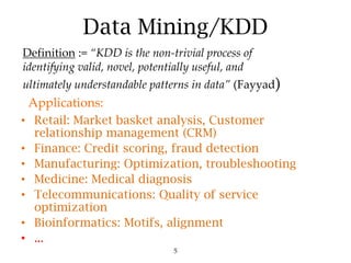

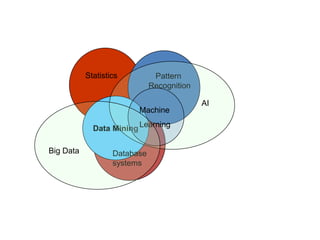


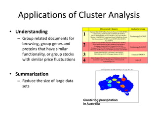


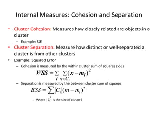
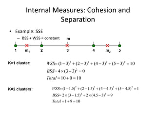


The document provides an overview of machine learning and data mining, highlighting their definitions, types, applications, and importance in various fields. Machine learning, a branch of artificial intelligence, focuses on predictive modeling, while data mining is concerned with discovering previously unknown patterns in data. Additionally, it discusses clustering techniques and algorithms, such as k-means and hierarchical clustering, outlining their processes, strengths, and limitations.


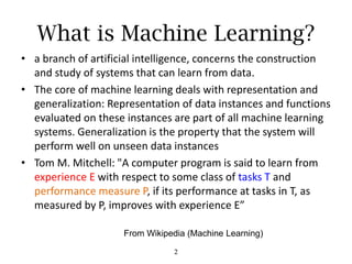
![[ML]-Unsupervised-learning_Unit2.ppt.pdf](https://cdn.slidesharecdn.com/ss_thumbnails/ml-unsupervised-learningunit2-230916145038-acbd0397-thumbnail.jpg?width=640&height=640&fit=bounds)

![Chapter#04[Part#01]K-Means Clusterig.pdf](https://cdn.slidesharecdn.com/ss_thumbnails/chapter04part01k-meansclusterig-250525201708-2d369307-thumbnail.jpg?width=640&height=640&fit=bounds)


![[DSC Europe 25] Slobodan Dolinic - Smart and Intelligent Green Region.pptx](https://cdn.slidesharecdn.com/ss_thumbnails/0bribinjsp6ghwtvsvor-2-sigre-slobodan-dolinic-260115093812-c9c10e90-thumbnail.jpg?width=640&height=640&fit=bounds)


