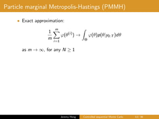
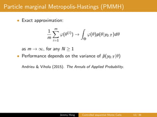
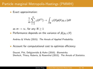
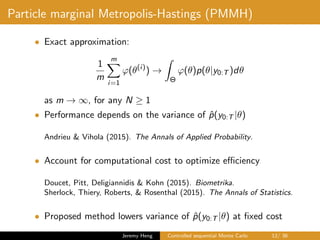
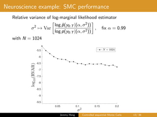
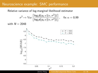
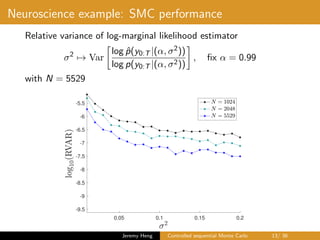
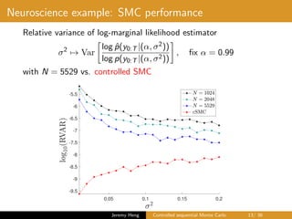
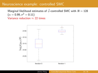
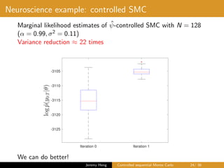
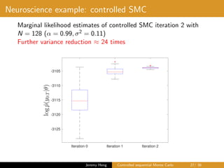
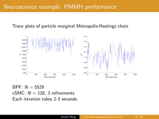
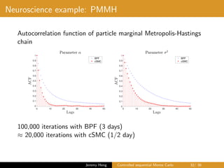
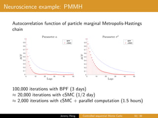
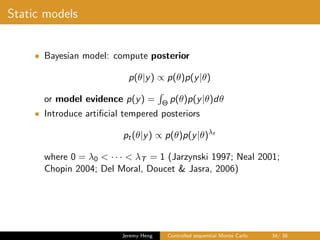
This document summarizes a presentation on controlled sequential Monte Carlo. It discusses state space models, sequential Monte Carlo, and particle marginal Metropolis-Hastings for parameter inference. Controlled sequential Monte Carlo is proposed to lower the variance of the marginal likelihood estimator compared to standard sequential Monte Carlo, improving the performance of parameter inference methods. The method is illustrated on a neuroscience example where it reduces variance for different particle sizes.
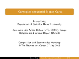


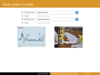
![State space models
X0
Latent Markov chain
X0 ∼ µ, Xt|Xt−1 ∼ ft(Xt−1, ·), t ∈ [1 : T]
Observations
Yt|X0:T ∼ gt(Xt, ·), t ∈ [0 : T]
Jeremy Heng Controlled sequential Monte Carlo 3/ 36](https://image.slidesharecdn.com/jobtalkgrips-180810050002/85/Controlled-sequential-Monte-Carlo-4-320.jpg)
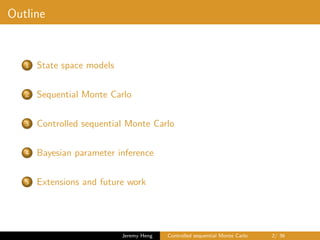
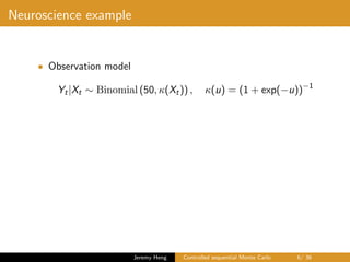
![State space models
…X0 X1 XT
Latent Markov chain
X0 ∼ µ, Xt|Xt−1 ∼ ft(Xt−1, ·), t ∈ [1 : T]
Observations
Yt|X0:T ∼ gt(Xt, ·), t ∈ [0 : T]
Jeremy Heng Controlled sequential Monte Carlo 3/ 36](https://image.slidesharecdn.com/jobtalkgrips-180810050002/85/Controlled-sequential-Monte-Carlo-5-320.jpg)
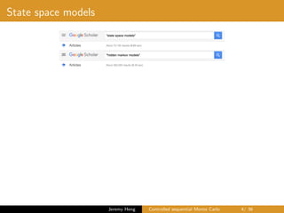
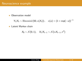
![State space models
…X0 X1 XT
Y0 Y1 YT…
Latent Markov chain
X0 ∼ µ, Xt|Xt−1 ∼ ft(Xt−1, ·), t ∈ [1 : T]
Observations
Yt|X0:T ∼ gt(Xt, ·), t ∈ [0 : T]
Jeremy Heng Controlled sequential Monte Carlo 3/ 36](https://image.slidesharecdn.com/jobtalkgrips-180810050002/85/Controlled-sequential-Monte-Carlo-6-320.jpg)
![State space models
…X0 X1 XT
Y0 Y1 YT…
✓
Latent Markov chain
X0 ∼ µθ, Xt|Xt−1 ∼ ft,θ(Xt−1, ·), t ∈ [1 : T]
Observations
Yt|X0:T ∼ gt,θ(Xt, ·), t ∈ [0 : T]
Jeremy Heng Controlled sequential Monte Carlo 3/ 36](https://image.slidesharecdn.com/jobtalkgrips-180810050002/85/Controlled-sequential-Monte-Carlo-7-320.jpg)


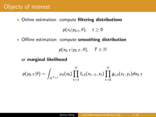
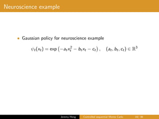
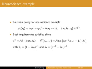
![Neuroscience example
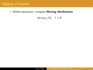
• Observation model
Yt|Xt ∼ Binomial (50, κ(Xt)) , κ(u) = (1 + exp(−u))−1
• Latent Markov chain
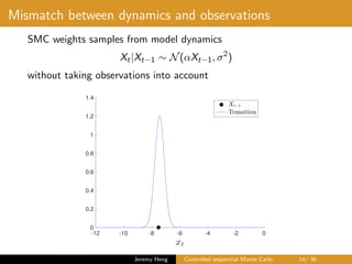
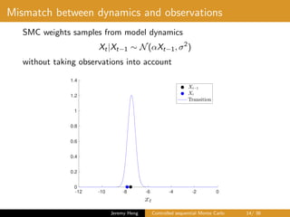
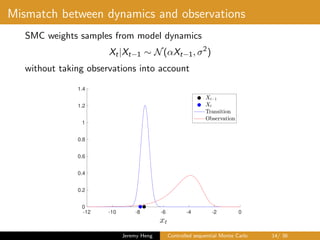
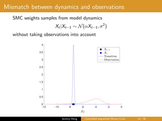
X0 ∼ N(0, 1), Xt|Xt−1 ∼ N(αXt−1, σ2
)
• Unknown parameters
θ = (α, σ2
) ∈ [0, 1] × (0, ∞)
Jeremy Heng Controlled sequential Monte Carlo 6/ 36](https://image.slidesharecdn.com/jobtalkgrips-180810050002/85/Controlled-sequential-Monte-Carlo-17-320.jpg)

![Sequential Monte Carlo
• Sequential Monte Carlo (SMC) aka bootstrap particle filter
(BPF) recursively simulates an interacting particle system of
size N
(X1
t , . . . , XN
t ), t ∈ [0 : T]
Del Moral (2004). Feynman-Kac formulae.
Jeremy Heng Controlled sequential Monte Carlo 8/ 36](https://image.slidesharecdn.com/jobtalkgrips-180810050002/85/Controlled-sequential-Monte-Carlo-22-320.jpg)
![Sequential Monte Carlo
• Sequential Monte Carlo (SMC) aka bootstrap particle filter
(BPF) recursively simulates an interacting particle system of
size N
(X1
t , . . . , XN
t ), t ∈ [0 : T]
• Unbiased and consistent marginal likelihood estimator
ˆp(y0:T |θ) =
T
t=0
1
N
N
n=1
gt,θ(Xn
t , yt)
Del Moral (2004). Feynman-Kac formulae.
Jeremy Heng Controlled sequential Monte Carlo 8/ 36](https://image.slidesharecdn.com/jobtalkgrips-180810050002/85/Controlled-sequential-Monte-Carlo-23-320.jpg)
![Sequential Monte Carlo
• Sequential Monte Carlo (SMC) aka bootstrap particle filter
(BPF) recursively simulates an interacting particle system of
size N
(X1
t , . . . , XN
t ), t ∈ [0 : T]
• Unbiased and consistent marginal likelihood estimator
ˆp(y0:T |θ) =
T
t=0
1
N
N
n=1
gt,θ(Xn
t , yt)
• Consistent approximation of smoothing distribution
1
N
N
n=1
ϕ(Xn
0:T ) → ϕ(x0:T )p(x0:T |y0:T , θ)dx0:T
as N → ∞
Del Moral (2004). Feynman-Kac formulae.
Jeremy Heng Controlled sequential Monte Carlo 8/ 36](https://image.slidesharecdn.com/jobtalkgrips-180810050002/85/Controlled-sequential-Monte-Carlo-24-320.jpg)
![Sequential Monte Carlo
…X0 X1 XT
Y0 Y1 YT…
✓
For time t = 0 and particle n ∈ [1 : N]
sample Xn
0 ∼ µθ
Jeremy Heng Controlled sequential Monte Carlo 9/ 36](https://image.slidesharecdn.com/jobtalkgrips-180810050002/85/Controlled-sequential-Monte-Carlo-25-320.jpg)
![Sequential Monte Carlo
…X0 X1 XT
Y0 Y1 YT…
✓
For time t = 0 and particle n ∈ [1 : N]
weight W n
0 ∝ g0,θ(Xn
0 , y0)
Jeremy Heng Controlled sequential Monte Carlo 9/ 36](https://image.slidesharecdn.com/jobtalkgrips-180810050002/85/Controlled-sequential-Monte-Carlo-26-320.jpg)
![Sequential Monte Carlo
…X0 X1 XT
Y0 Y1 YT…
✓
X
X
X
For time t = 0 and particle n ∈ [1 : N]
sample ancestor An
0 ∼ R W 1
0 , . . . , W N
0 , resampled particle: X
An
0
0
Jeremy Heng Controlled sequential Monte Carlo 9/ 36](https://image.slidesharecdn.com/jobtalkgrips-180810050002/85/Controlled-sequential-Monte-Carlo-27-320.jpg)
![Sequential Monte Carlo
…X0 X1 XT
Y0 Y1 YT…
✓
X
X
X
For time t = 1 and particle n ∈ [1 : N]
sample Xn
1 ∼ f1,θ(X
An
0
0 , ·)
Jeremy Heng Controlled sequential Monte Carlo 9/ 36](https://image.slidesharecdn.com/jobtalkgrips-180810050002/85/Controlled-sequential-Monte-Carlo-28-320.jpg)
![Sequential Monte Carlo
…X0 X1 XT
Y0 Y1 YT…
✓
X
X
X
For time t = 1 and particle n ∈ [1 : N]
weight W n
1 ∝ g1,θ(Xn
1 , y1)
Jeremy Heng Controlled sequential Monte Carlo 9/ 36](https://image.slidesharecdn.com/jobtalkgrips-180810050002/85/Controlled-sequential-Monte-Carlo-29-320.jpg)
![Sequential Monte Carlo
…X0 X1 XT
Y0 Y1 YT…
✓
X
X
X X
For time t = 1 and particle n ∈ [1 : N]
sample ancestor An
1 ∼ R W 1
1 , . . . , W N
1 , resampled particle: X
An
1
1
Jeremy Heng Controlled sequential Monte Carlo 9/ 36](https://image.slidesharecdn.com/jobtalkgrips-180810050002/85/Controlled-sequential-Monte-Carlo-30-320.jpg)
![Sequential Monte Carlo
…X0 X1 XT
Y0 Y1 YT…
✓
X
X
X X
X
X
X
Repeat for time t ∈ [2 : T].
Jeremy Heng Controlled sequential Monte Carlo 9/ 36](https://image.slidesharecdn.com/jobtalkgrips-180810050002/85/Controlled-sequential-Monte-Carlo-31-320.jpg)
![Sequential Monte Carlo
…X0 X1 XT
Y0 Y1 YT…
✓
X
X
X X
X
X
X
Repeat for time t ∈ [2 : T]. Note this is for a given θ!
Jeremy Heng Controlled sequential Monte Carlo 9/ 36](https://image.slidesharecdn.com/jobtalkgrips-180810050002/85/Controlled-sequential-Monte-Carlo-32-320.jpg)

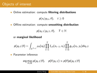
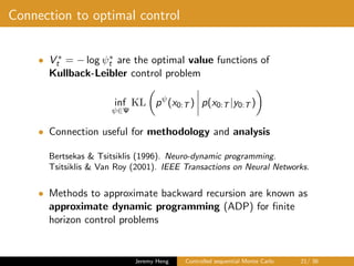
![Optimal dynamics
• Fix θ and suppress notational dependency
• Sampling from smoothing distribution p(x0:T |y0:T )
X0 ∼ p(x0|y0:T ), Xt|Xt−1 ∼ p(xt|xt−1, yt:T ), t ∈ [1 : T]
Jeremy Heng Controlled sequential Monte Carlo 15/ 36](https://image.slidesharecdn.com/jobtalkgrips-180810050002/85/Controlled-sequential-Monte-Carlo-49-320.jpg)
![Optimal dynamics
• Fix θ and suppress notational dependency
• Sampling from smoothing distribution p(x0:T |y0:T )
X0 ∼ p(x0|y0:T ), Xt|Xt−1 ∼ p(xt|xt−1, yt:T ), t ∈ [1 : T]
• Define backward information filter ψ∗
t (xt) = p(yt:T |xt),
then
p(x0|y0:T ) =
µ(x0)ψ∗
0(x0)
µ(ψ∗
0)
with µ(ψ∗
0) = X ψ∗
0(x0)µ(x0)dx0, and
p(xt|xt−1, yt:T ) =
ft(xt−1, xt)ψ∗
t (xt)
ft(ψ∗
t )(xt−1)
with ft(ψ∗
t )(xt−1) = X ψ∗
t (xt)ft(xt−1, xt)dxt
Jeremy Heng Controlled sequential Monte Carlo 15/ 36](https://image.slidesharecdn.com/jobtalkgrips-180810050002/85/Controlled-sequential-Monte-Carlo-50-320.jpg)
![Controlled state space model
• Given a policy
ψ = (ψ0, . . . , ψT )
i.e. positive and bounded functions
• Construct ψ-controlled dynamics
X0 ∼ µψ
, Xt|Xt−1 ∼ f ψ
t (Xt−1, ·), t ∈ [1 : T]
where
µψ
(x0) =
µ(x0)ψ0(x0)
µ(ψ0)
, f ψ
t (xt−1, xt) =
ft(xt−1, xt)ψt(xt)
ft(ψt)(xt−1)
Jeremy Heng Controlled sequential Monte Carlo 16/ 36](https://image.slidesharecdn.com/jobtalkgrips-180810050002/85/Controlled-sequential-Monte-Carlo-52-320.jpg)
![Controlled state space model
• Given a policy
ψ = (ψ0, . . . , ψT )
i.e. positive and bounded functions
• Construct ψ-controlled dynamics
X0 ∼ µψ
, Xt|Xt−1 ∼ f ψ
t (Xt−1, ·), t ∈ [1 : T]
where
µψ
(x0) =
µ(x0)ψ0(x0)
µ(ψ0)
, f ψ
t (xt−1, xt) =
ft(xt−1, xt)ψt(xt)
ft(ψt)(xt−1)
• Introducing ψ-controlled observation model
Yt|X0:T ∼ gψ
t (Xt, ·), t ∈ [0 : T]
gives a ψ-controlled state space model
Jeremy Heng Controlled sequential Monte Carlo 16/ 36](https://image.slidesharecdn.com/jobtalkgrips-180810050002/85/Controlled-sequential-Monte-Carlo-53-320.jpg)
![Controlled state space model
• Define controlled observation densities (gψ
0 , . . . , gψ
T ) so
that
pψ
(x0:T |y0:T ) = p(x0:T |y0:T ), pψ
(y0:T ) = p(y0:T )
• Achieved with
gψ
0 (x0, y0) =
µ(ψ0)g0(x0, y0)f1(ψ1)(x0)
ψ0(x0)
,
gψ
t (xt, yt) =
gt(xt, yt)ft+1(ψt+1)(xt)
ψt(xt)
, t ∈ [1 : T − 1],
gψ
T (xT , yT ) =
gT (xT , yT )
ψT (xT )
Jeremy Heng Controlled sequential Monte Carlo 17/ 36](https://image.slidesharecdn.com/jobtalkgrips-180810050002/85/Controlled-sequential-Monte-Carlo-55-320.jpg)
![Controlled state space model
• Define controlled observation densities (gψ
0 , . . . , gψ
T ) so
that
pψ
(x0:T |y0:T ) = p(x0:T |y0:T ), pψ
(y0:T ) = p(y0:T )
• Achieved with
gψ
0 (x0, y0) =
µ(ψ0)g0(x0, y0)f1(ψ1)(x0)
ψ0(x0)
,
gψ
t (xt, yt) =
gt(xt, yt)ft+1(ψt+1)(xt)
ψt(xt)
, t ∈ [1 : T − 1],
gψ
T (xT , yT ) =
gT (xT , yT )
ψT (xT )
• Requirements on policy ψ
– Evaluating gψ
t tractable
Jeremy Heng Controlled sequential Monte Carlo 17/ 36](https://image.slidesharecdn.com/jobtalkgrips-180810050002/85/Controlled-sequential-Monte-Carlo-56-320.jpg)
![Controlled state space model
• Define controlled observation densities (gψ
0 , . . . , gψ
T ) so
that
pψ
(x0:T |y0:T ) = p(x0:T |y0:T ), pψ
(y0:T ) = p(y0:T )
• Achieved with
gψ
0 (x0, y0) =
µ(ψ0)g0(x0, y0)f1(ψ1)(x0)
ψ0(x0)
,
gψ
t (xt, yt) =
gt(xt, yt)ft+1(ψt+1)(xt)
ψt(xt)
, t ∈ [1 : T − 1],
gψ
T (xT , yT ) =
gT (xT , yT )
ψT (xT )
• Requirements on policy ψ
– Evaluating gψ
t tractable
– Sampling µψ and f ψ
t feasible
Jeremy Heng Controlled sequential Monte Carlo 17/ 36](https://image.slidesharecdn.com/jobtalkgrips-180810050002/85/Controlled-sequential-Monte-Carlo-57-320.jpg)
![Controlled SMC
• Construct ψ-controlled SMC as SMC applied to ψ-controlled
state space model
X0 ∼ µψ
, Xt|Xt−1 ∼ f ψ
t (Xt−1, ·), t ∈ [1 : T]
Yt|X0:T ∼ gψ
t (Xt, ·), t ∈ [0 : T]
Jeremy Heng Controlled sequential Monte Carlo 19/ 36](https://image.slidesharecdn.com/jobtalkgrips-180810050002/85/Controlled-sequential-Monte-Carlo-60-320.jpg)
![Controlled SMC
• Construct ψ-controlled SMC as SMC applied to ψ-controlled
state space model
X0 ∼ µψ
, Xt|Xt−1 ∼ f ψ
t (Xt−1, ·), t ∈ [1 : T]
Yt|X0:T ∼ gψ
t (Xt, ·), t ∈ [0 : T]
• Unbiased and consistent marginal likelihood estimator
ˆpψ
(y0:T ) =
T
t=0
1
N
N
n=1
gψ
t (Xn
t , yt)
Jeremy Heng Controlled sequential Monte Carlo 19/ 36](https://image.slidesharecdn.com/jobtalkgrips-180810050002/85/Controlled-sequential-Monte-Carlo-61-320.jpg)
![Controlled SMC
• Construct ψ-controlled SMC as SMC applied to ψ-controlled
state space model
X0 ∼ µψ
, Xt|Xt−1 ∼ f ψ
t (Xt−1, ·), t ∈ [1 : T]
Yt|X0:T ∼ gψ
t (Xt, ·), t ∈ [0 : T]
• Unbiased and consistent marginal likelihood estimator
ˆpψ
(y0:T ) =
T
t=0
1
N
N
n=1
gψ
t (Xn
t , yt)
• Consistent approximation of smoothing distribution
1
N
N
n=1
ϕ(Xn
0:T ) → ϕ(x0:T )p(x0:T |y0:T )dx0:T
as N → ∞
Jeremy Heng Controlled sequential Monte Carlo 19/ 36](https://image.slidesharecdn.com/jobtalkgrips-180810050002/85/Controlled-sequential-Monte-Carlo-62-320.jpg)
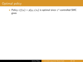
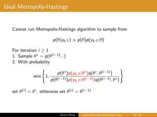
![Optimal policy
• Policy ψ∗
t (xt) = p(yt:T |xt) is optimal since ψ∗-controlled SMC
gives
• ψ∗-controlled SMC gives independent samples from
smoothing distribution
Xn
0:T ∼ p(x0:T |y0:T ), n ∈ [1 : N],
and zero variance estimator of marginal likelihood for any
N ≥ 1
ˆpψ∗
(y0:T ) = p(y0:T )
Jeremy Heng Controlled sequential Monte Carlo 20/ 36](https://image.slidesharecdn.com/jobtalkgrips-180810050002/85/Controlled-sequential-Monte-Carlo-64-320.jpg)
![Optimal policy
• Policy ψ∗
t (xt) = p(yt:T |xt) is optimal since ψ∗-controlled SMC
gives
• ψ∗-controlled SMC gives independent samples from
smoothing distribution
Xn
0:T ∼ p(x0:T |y0:T ), n ∈ [1 : N],
and zero variance estimator of marginal likelihood for any
N ≥ 1
ˆpψ∗
(y0:T ) = p(y0:T )
• (Proposition 1) Optimal policy satisfies backward recursion
ψ∗
T (xT ) = gT (xT , yT ),
ψ∗
t (xt) = gt(xt, yt)ft+1(ψ∗
t+1)(xt), t ∈ [T − 1 : 0]
Jeremy Heng Controlled sequential Monte Carlo 20/ 36](https://image.slidesharecdn.com/jobtalkgrips-180810050002/85/Controlled-sequential-Monte-Carlo-65-320.jpg)
![Optimal policy
• Policy ψ∗
t (xt) = p(yt:T |xt) is optimal since ψ∗-controlled SMC
gives
• ψ∗-controlled SMC gives independent samples from
smoothing distribution
Xn
0:T ∼ p(x0:T |y0:T ), n ∈ [1 : N],
and zero variance estimator of marginal likelihood for any
N ≥ 1
ˆpψ∗
(y0:T ) = p(y0:T )
• (Proposition 1) Optimal policy satisfies backward recursion
ψ∗
T (xT ) = gT (xT , yT ),
ψ∗
t (xt) = gt(xt, yt)ft+1(ψ∗
t+1)(xt), t ∈ [T − 1 : 0]
• Backward recursion typically intractable but can be
approximated
Jeremy Heng Controlled sequential Monte Carlo 20/ 36](https://image.slidesharecdn.com/jobtalkgrips-180810050002/85/Controlled-sequential-Monte-Carlo-66-320.jpg)
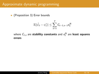
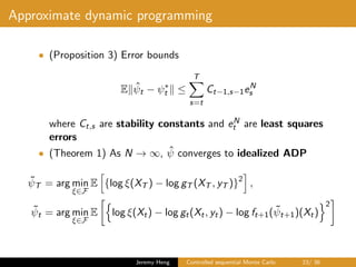
![Approximate dynamic programming
• First run standard SMC to get (Xn
0 , . . . , Xn
T ), n ∈ [1 : N]
Jeremy Heng Controlled sequential Monte Carlo 22/ 36](https://image.slidesharecdn.com/jobtalkgrips-180810050002/85/Controlled-sequential-Monte-Carlo-70-320.jpg)
![Approximate dynamic programming
• First run standard SMC to get (Xn
0 , . . . , Xn
T ), n ∈ [1 : N]
• For time T, approximate
ψ∗
T (xT ) = gT (xT , yT )
by least squares
ˆψT = arg min
ξ∈F
N
n=1
{log ξ(Xn
T ) − log gT (Xn
T , yT )}2
Jeremy Heng Controlled sequential Monte Carlo 22/ 36](https://image.slidesharecdn.com/jobtalkgrips-180810050002/85/Controlled-sequential-Monte-Carlo-71-320.jpg)
![Approximate dynamic programming
• First run standard SMC to get (Xn
0 , . . . , Xn
T ), n ∈ [1 : N]
• For time T, approximate
ψ∗
T (xT ) = gT (xT , yT )
by least squares
ˆψT = arg min
ξ∈F
N
n=1
{log ξ(Xn
T ) − log gT (Xn
T , yT )}2
• For t ∈ [T − 1 : 0], approximate
ψ∗
t (xt) = gt(xt, yt)ft+1(ψ∗
t+1)(xt)
by least squares and ψ∗
t+1 ≈ ˆψt+1
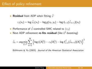
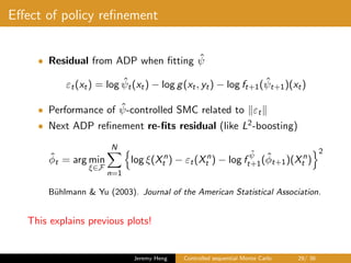
ˆψt = arg min
ξ∈F
N
n=1
log ξ(Xn
t ) − log gt(Xn
t , yt) − log ft+1( ˆψt+1)(Xn
t )
2
Jeremy Heng Controlled sequential Monte Carlo 22/ 36](https://image.slidesharecdn.com/jobtalkgrips-180810050002/85/Controlled-sequential-Monte-Carlo-72-320.jpg)
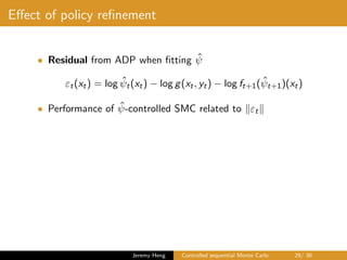
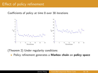
![Policy refinement
• Current policy ˆψ defines the dynamics
X0 ∼ µ
ˆψ
, Xt|Xt−1 ∼ f
ˆψ
t (Xt−1, ·), t ∈ [1 : T]
Jeremy Heng Controlled sequential Monte Carlo 25/ 36](https://image.slidesharecdn.com/jobtalkgrips-180810050002/85/Controlled-sequential-Monte-Carlo-77-320.jpg)
![Policy refinement
• Current policy ˆψ defines the dynamics
X0 ∼ µ
ˆψ
, Xt|Xt−1 ∼ f
ˆψ
t (Xt−1, ·), t ∈ [1 : T]
• Further control these dynamics with policy φ = (φ0, . . . φT )
X0 ∼ µ
ˆψ
φ
, Xt|Xt−1 ∼ f
ˆψ
t
φ
(Xt−1, ·), t ∈ [1 : T]
Jeremy Heng Controlled sequential Monte Carlo 25/ 36](https://image.slidesharecdn.com/jobtalkgrips-180810050002/85/Controlled-sequential-Monte-Carlo-78-320.jpg)
![Policy refinement
• Current policy ˆψ defines the dynamics
X0 ∼ µ
ˆψ
, Xt|Xt−1 ∼ f
ˆψ
t (Xt−1, ·), t ∈ [1 : T]
• Further control these dynamics with policy φ = (φ0, . . . φT )
X0 ∼ µ
ˆψ
φ
, Xt|Xt−1 ∼ f
ˆψ
t
φ
(Xt−1, ·), t ∈ [1 : T]
• Equivalent to controlling model dynamics µ and ft with policy
ˆψ · φ = ( ˆψ0 · φ0, . . . , ˆψT · φT )
Jeremy Heng Controlled sequential Monte Carlo 25/ 36](https://image.slidesharecdn.com/jobtalkgrips-180810050002/85/Controlled-sequential-Monte-Carlo-79-320.jpg)
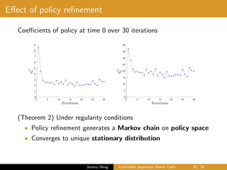
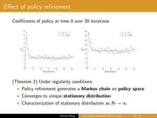
![Policy refinement
• (Proposition 1) Optimal refinement of φ∗ current policy ˆψ
φ∗
T (xT ) = g
ˆψ
T (xT , yT ),
φ∗
t (xt) = g
ˆψ
t (xt, yt)f
ˆψ
t+1(φ∗
t+1)(xt), t ∈ [T − 1 : 0]
Jeremy Heng Controlled sequential Monte Carlo 26/ 36](https://image.slidesharecdn.com/jobtalkgrips-180810050002/85/Controlled-sequential-Monte-Carlo-80-320.jpg)
![Policy refinement
• (Proposition 1) Optimal refinement of φ∗ current policy ˆψ
φ∗
T (xT ) = g
ˆψ
T (xT , yT ),
φ∗
t (xt) = g
ˆψ
t (xt, yt)f
ˆψ
t+1(φ∗
t+1)(xt), t ∈ [T − 1 : 0]
• Optimal policy ψ∗ = ˆψ · φ∗
Jeremy Heng Controlled sequential Monte Carlo 26/ 36](https://image.slidesharecdn.com/jobtalkgrips-180810050002/85/Controlled-sequential-Monte-Carlo-81-320.jpg)
![Policy refinement
• (Proposition 1) Optimal refinement of φ∗ current policy ˆψ
φ∗
T (xT ) = g
ˆψ
T (xT , yT ),
φ∗
t (xt) = g
ˆψ
t (xt, yt)f
ˆψ
t+1(φ∗
t+1)(xt), t ∈ [T − 1 : 0]
• Optimal policy ψ∗ = ˆψ · φ∗
• Approximate backward recursion to obtain ˆφ ≈ φ∗
– using particles from ˆψ-controlled SMC
– same function class F
Jeremy Heng Controlled sequential Monte Carlo 26/ 36](https://image.slidesharecdn.com/jobtalkgrips-180810050002/85/Controlled-sequential-Monte-Carlo-82-320.jpg)
![Policy refinement
• (Proposition 1) Optimal refinement of φ∗ current policy ˆψ
φ∗
T (xT ) = g
ˆψ
T (xT , yT ),
φ∗
t (xt) = g
ˆψ
t (xt, yt)f
ˆψ
t+1(φ∗
t+1)(xt), t ∈ [T − 1 : 0]
• Optimal policy ψ∗ = ˆψ · φ∗
• Approximate backward recursion to obtain ˆφ ≈ φ∗
– using particles from ˆψ-controlled SMC
– same function class F
• Run controlled SMC with refined policy ˆψ · ˆφ
Jeremy Heng Controlled sequential Monte Carlo 26/ 36](https://image.slidesharecdn.com/jobtalkgrips-180810050002/85/Controlled-sequential-Monte-Carlo-83-320.jpg)


![제 23회 보아즈(BOAZ) 빅데이터 컨퍼런스 - [MBOAX] : ABSA를 활용한 소비자 반응 분석 기반 운영 효율화 대시보드 설계](https://cdn.slidesharecdn.com/ss_thumbnails/3-1boaz23rdconferencemboax-260203102709-9d519923-thumbnail.jpg?width=640&height=640&fit=bounds)
