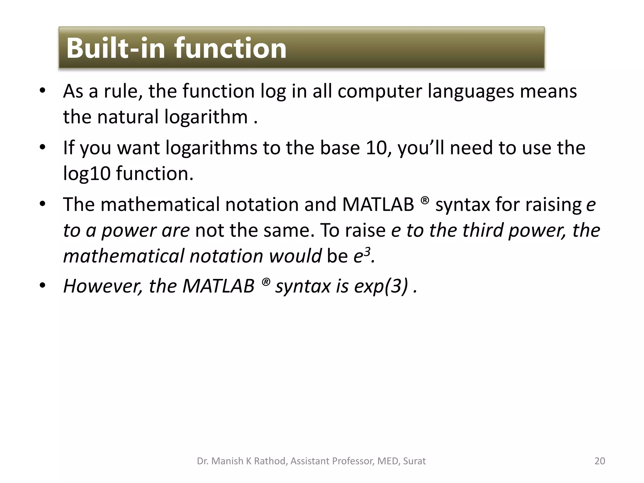
The document discusses MATLAB, including that it is a technical computing environment for numeric computation, graphics, and programming. It provides built-in functions for tasks like mathematical operations, data analysis, and trigonometric functions. User-defined functions in MATLAB allow repeating groups of commands to be stored and called by name, improving efficiency. Help tools are available to understand MATLAB functions and syntax.


![• The size function is an example of a function that returns
two outputs, which are stored in a single array. It determines
the number of rows and columns in a matrix. Thus,
d = [1, 2, 3; 4, 5, 6];
f = size(d) %returns the 1 X 2 result matrix
f = 2 3
• You can also assign variable names to each of the answers by
representing the left-hand side of the assignment statement
as a matrix. For example,
[rows,cols] = size(d)
rows =
2
cols =
3 16
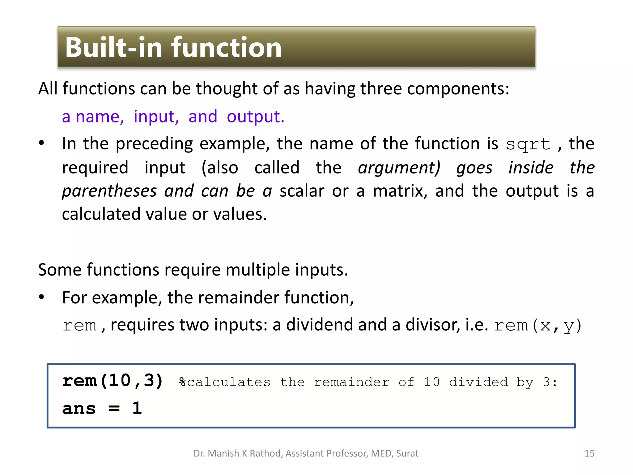
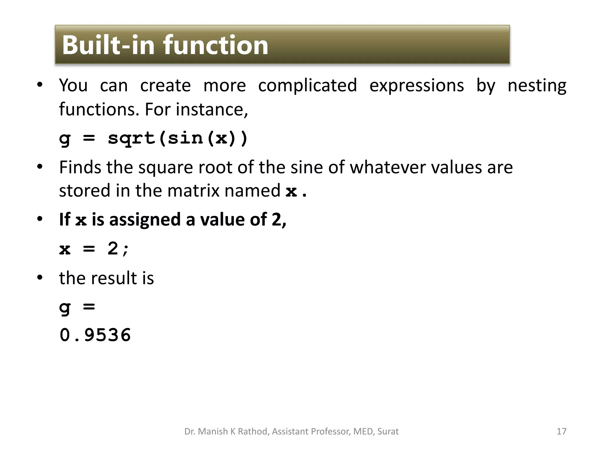
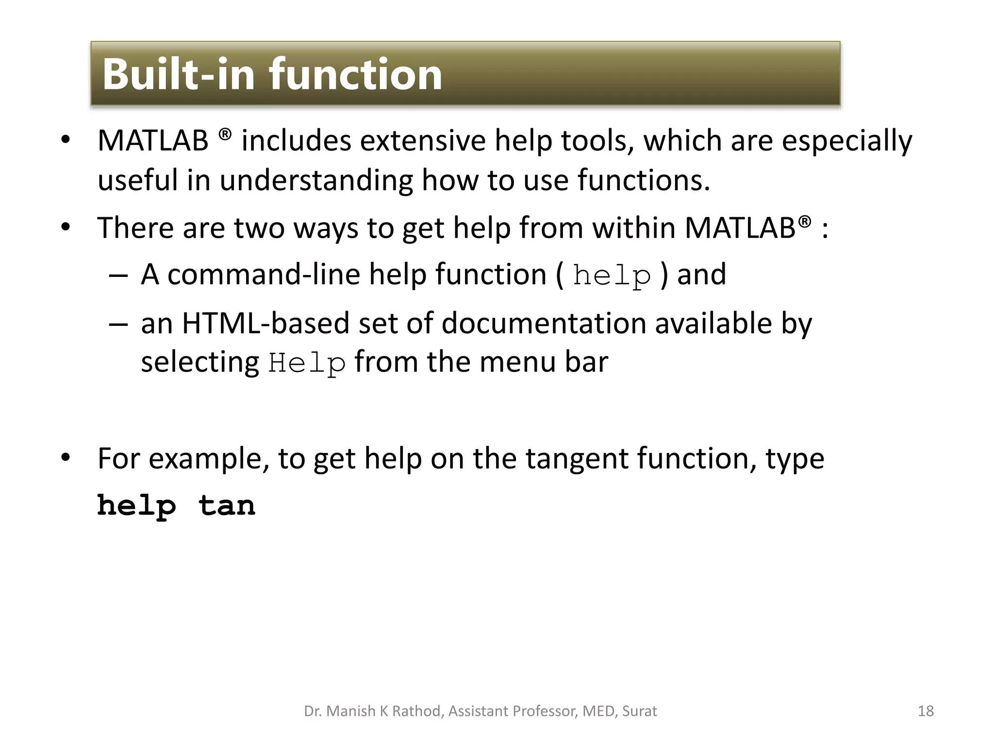
Built-in function
Dr. Manish K Rathod, Assistant Professor, MED, Surat](https://image.slidesharecdn.com/gettingstartmatlabbvm1-221215061824-4faa6455/75/Getting_Start_MATLAB_BVM1-pptx-16-2048.jpg)
![24
DATA ANALYSIS FUNCTIONS
• max(x)
Finds the largest value in a vector x.
x[1, 5, 3];
max(x)
ans =
5
If x[1, 5, 3; 2, 4, 6];…..????
• [a,b]=max(x)
Finds both the largest value in a vector x and its location in vector x.
x[1, 5, 3];
[a,b]= max(x)
a =
5
b =
2
Dr. Manish K Rathod, Assistant Professor, MED, Surat](https://image.slidesharecdn.com/gettingstartmatlabbvm1-221215061824-4faa6455/75/Getting_Start_MATLAB_BVM1-pptx-24-2048.jpg)
![25
DATA ANALYSIS FUNCTIONS
• max(x,y)
Creates a matrix the same size as x and y. (Both x and y must
have the same number of rows and columns.) Each element in
the resulting matrix contains the maximum value from the
corresponding positions in x and y.
x[1, 5, 3; 2, 4, 6]; y[10,2,4; 1, 8, 7];
max(x,y)
• Same as min(x);
[a,b]=min(x);
min(x,y)
Dr. Manish K Rathod, Assistant Professor, MED, Surat](https://image.slidesharecdn.com/gettingstartmatlabbvm1-221215061824-4faa6455/75/Getting_Start_MATLAB_BVM1-pptx-25-2048.jpg)
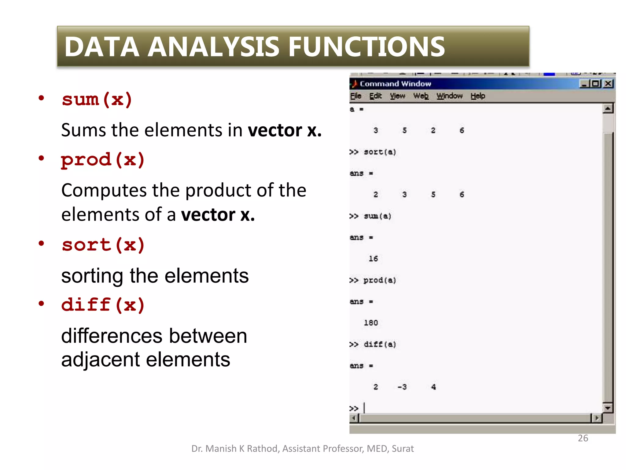
![27
DATA ANALYSIS FUNCTIONS
• cumsum(x)
Computes a vector of the same size as, and containing
cumulative sums of the elements of, a vector x.
For example, if x = [1 5 3], the resulting vector is x=[1 6 9].
• cumprod(x)
Computes a vector of the same size as, and containing
cumulative products of the elements of, a vector x .
For example, if x = [1 5 3], the resulting vector is x=[1 5 15].
• sortrows(x,n)
Sorts the rows in a matrix on the basis of the values in column
n. If n is negative, the values are sorted in descending order. If
n is not specified, the default column used as the basis for
sorting is column 1.
Dr. Manish K Rathod, Assistant Professor, MED, Surat](https://image.slidesharecdn.com/gettingstartmatlabbvm1-221215061824-4faa6455/75/Getting_Start_MATLAB_BVM1-pptx-27-2048.jpg)
![28
DATA ANALYSIS FUNCTIONS
skating_results = [ 1.0000 42.0930
2.0000 42.0890
3.0000 41.9350
4.0000 42.4970
5.0000 42.0020]
>> sortrows(skating_results)
>> sortrows(skating_results,2)
>> sortrows(skating_results,-2)
Dr. Manish K Rathod, Assistant Professor, MED, Surat](https://image.slidesharecdn.com/gettingstartmatlabbvm1-221215061824-4faa6455/75/Getting_Start_MATLAB_BVM1-pptx-28-2048.jpg)
![33
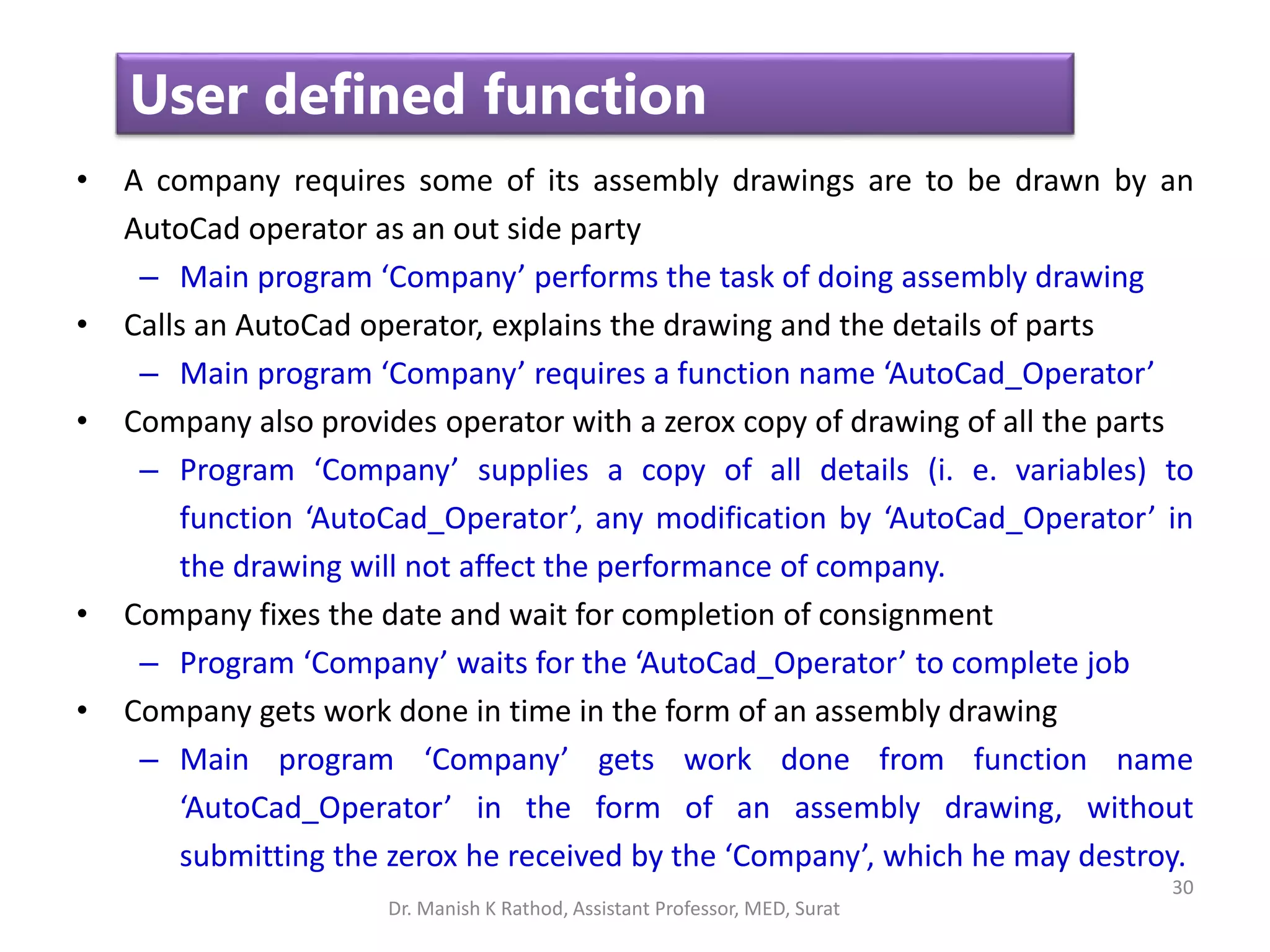
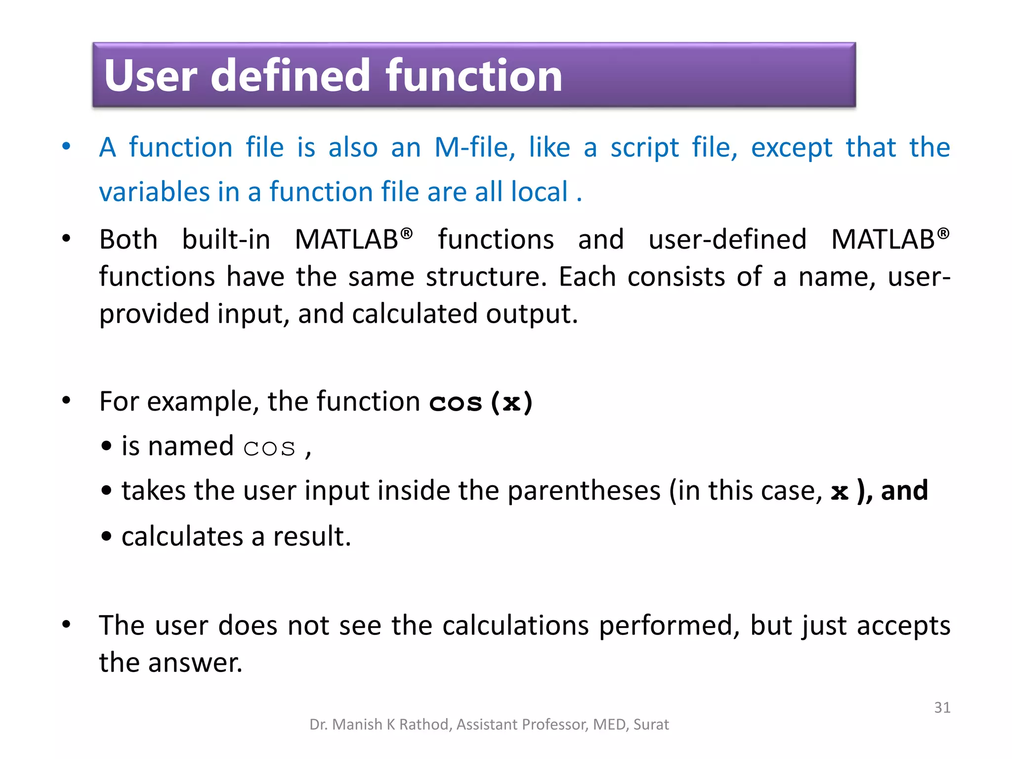
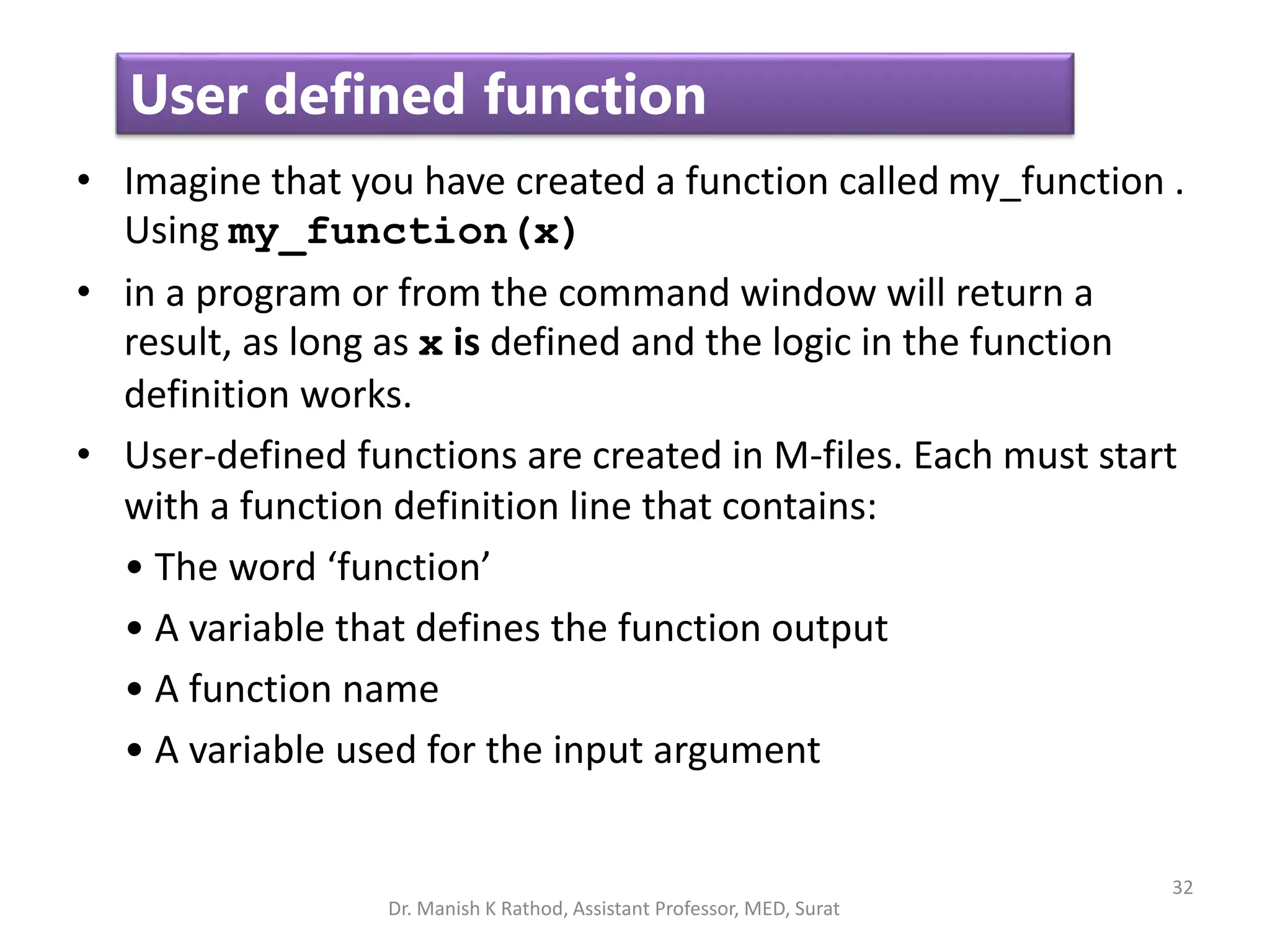
User defined function
• For example,
function [output variables] = my_function(x)
• The first word, function, is mandatory, and tells MATLAB this m-
file in a function file.
• On the lefthand side of the equals sign is a list of the output
variables that the function will return. When there is more than
one output variable, then they are enclosed in square brackets.
• On the righthand side of the equals sign is the name of the
function. The name used to save a function file must match the
function name.
• Lastly, within the round brackets after the function name, is a
comma separated list of the input variables.
Dr. Manish K Rathod, Assistant Professor, MED, Surat](https://image.slidesharecdn.com/gettingstartmatlabbvm1-221215061824-4faa6455/75/Getting_Start_MATLAB_BVM1-pptx-33-2048.jpg)
![38
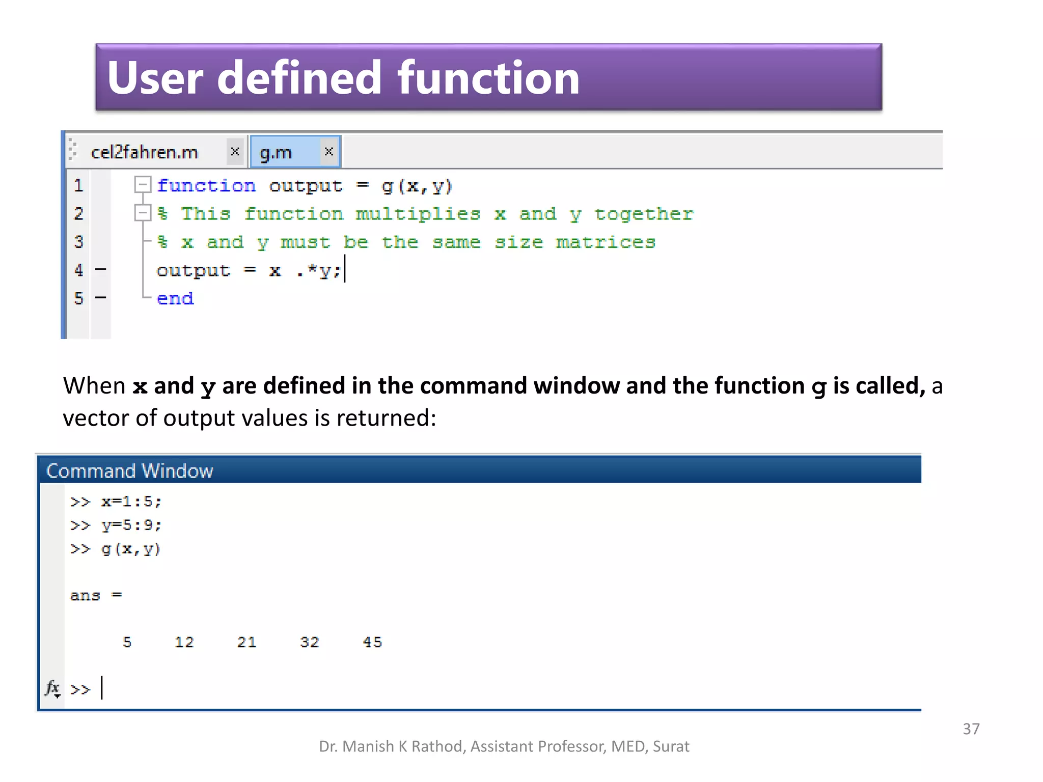
User defined function
• You can also create functions that return more than one output
variable. Make the output a matrix of answers instead of a single
variable
function [dist, vel, accel] = motion(t)
% This function calculates the distance, velocity, and
% acceleration of a particular car for a given value of t
% assuming all 3 parameters are initially 0.
accel = 0.5 .*t;
vel = t.^2/4;
dist = t.^3/12;
• Once saved as motion in the current folder, you can use the
function to find values of distance , velocity , and acceleration at
specified times:
Dr. Manish K Rathod, Assistant Professor, MED, Surat](https://image.slidesharecdn.com/gettingstartmatlabbvm1-221215061824-4faa6455/75/Getting_Start_MATLAB_BVM1-pptx-38-2048.jpg)
![39
User defined function
[distance, velocity, acceleration] = motion(10)
distance =
83.33
velocity =
25
acceleration =
5
• If you call the motion function without specifying all three outputs,
only the first output will be returned:
motion(10)
ans =
83.333
Dr. Manish K Rathod, Assistant Professor, MED, Surat](https://image.slidesharecdn.com/gettingstartmatlabbvm1-221215061824-4faa6455/75/Getting_Start_MATLAB_BVM1-pptx-39-2048.jpg)


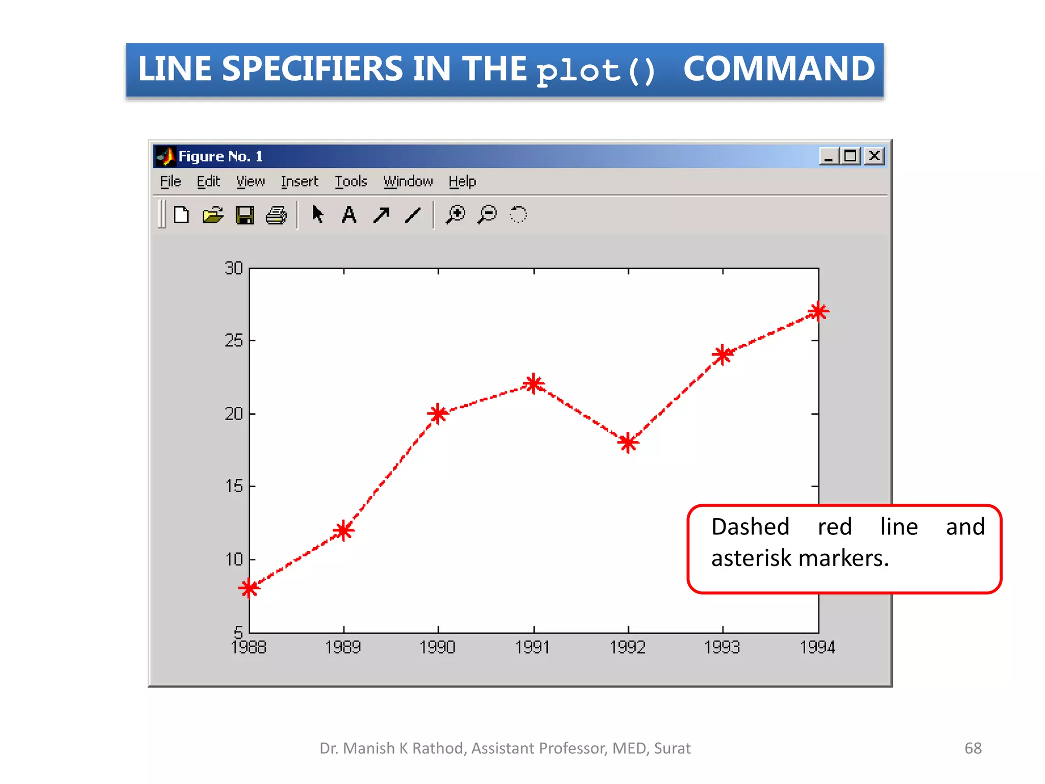
![Year
Sales (M)
1988 1989 1990 1991 1992 1993 1994
127 130 136 145 158 178 211
>> year = [1988:1:1994];
>> sales = [127, 130, 136, 145, 158, 178, 211];
>> plot(year,sales,'--r*')
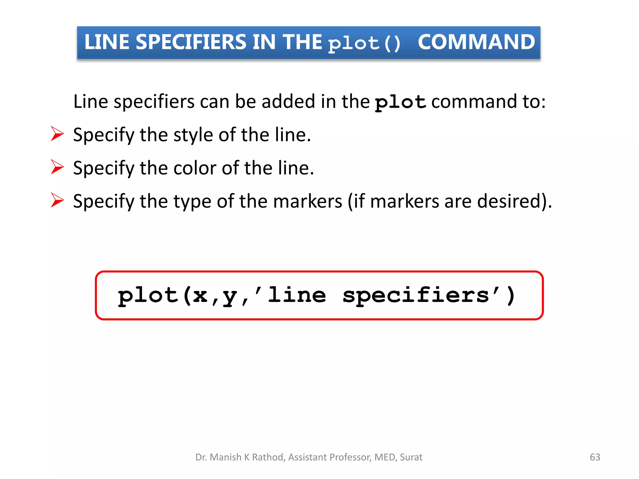
Line Specifiers:
dashed red line and
asterisk markers.
LINE SPECIFIERS IN THE plot() COMMAND
Dr. Manish K Rathod, Assistant Professor, MED, Surat 67](https://image.slidesharecdn.com/gettingstartmatlabbvm1-221215061824-4faa6455/75/Getting_Start_MATLAB_BVM1-pptx-67-2048.jpg)
![4
2
x
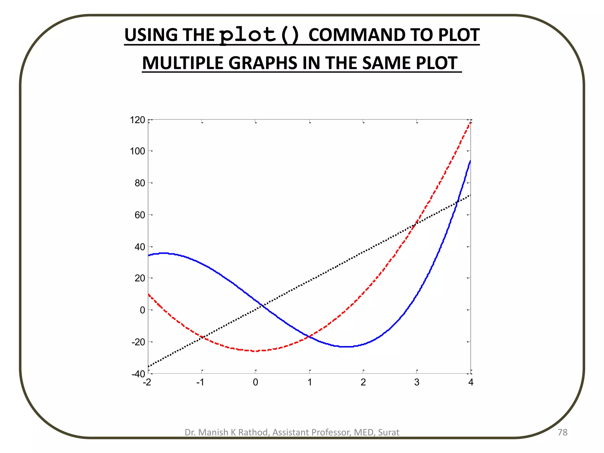
Plot of the function, and its first and second derivatives, for
, all in the same plot.
10
26
3 3
x
x
y
4
2
x
x = [-2:0.01:4];
y = 3*x.^3-26*x+6;
yd = 9*x.^2-26;
ydd = 18*x;
plot(x,y,'-b',x,yd,'--r',x,ydd,':k')
vector x with the domain of the function.
Vector y with the function value at each x.
4
2
x
Vector yd with values of the first derivative.
Vector ydd with values of the second derivative.
Create three graphs, y vs. x (solid blue line), yd vs.
x (dashed red line), and ydd vs. x (dotted black
line) in the same figure.
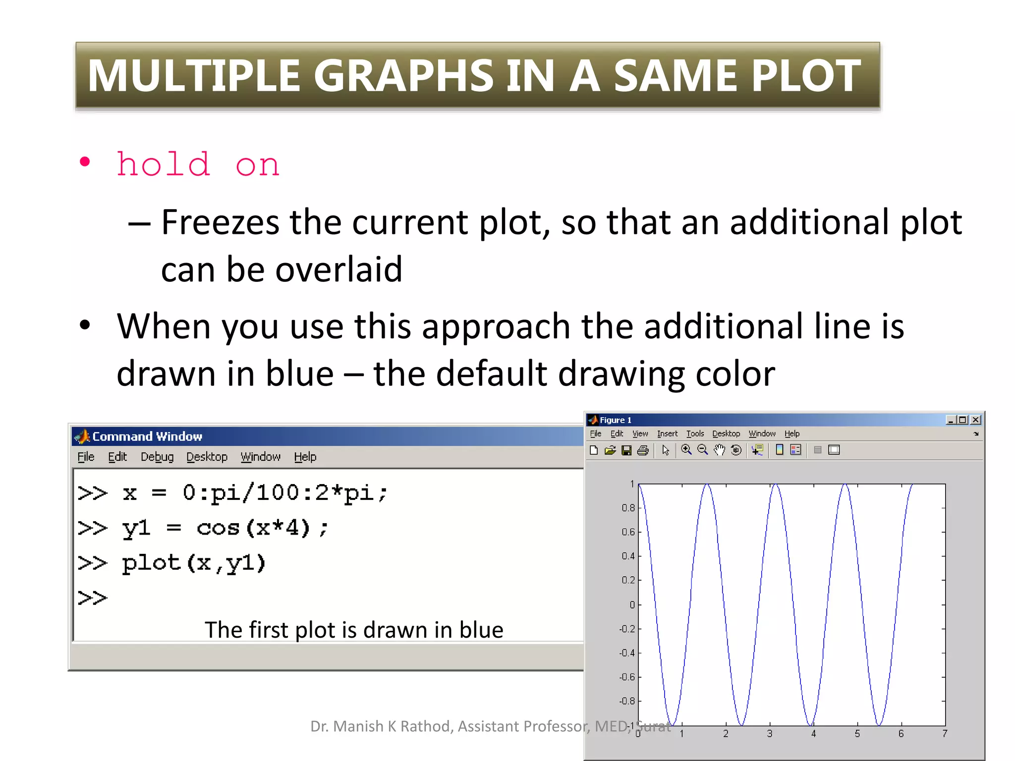
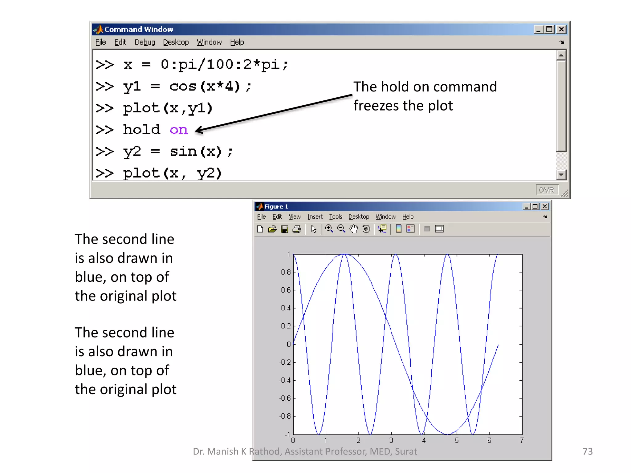
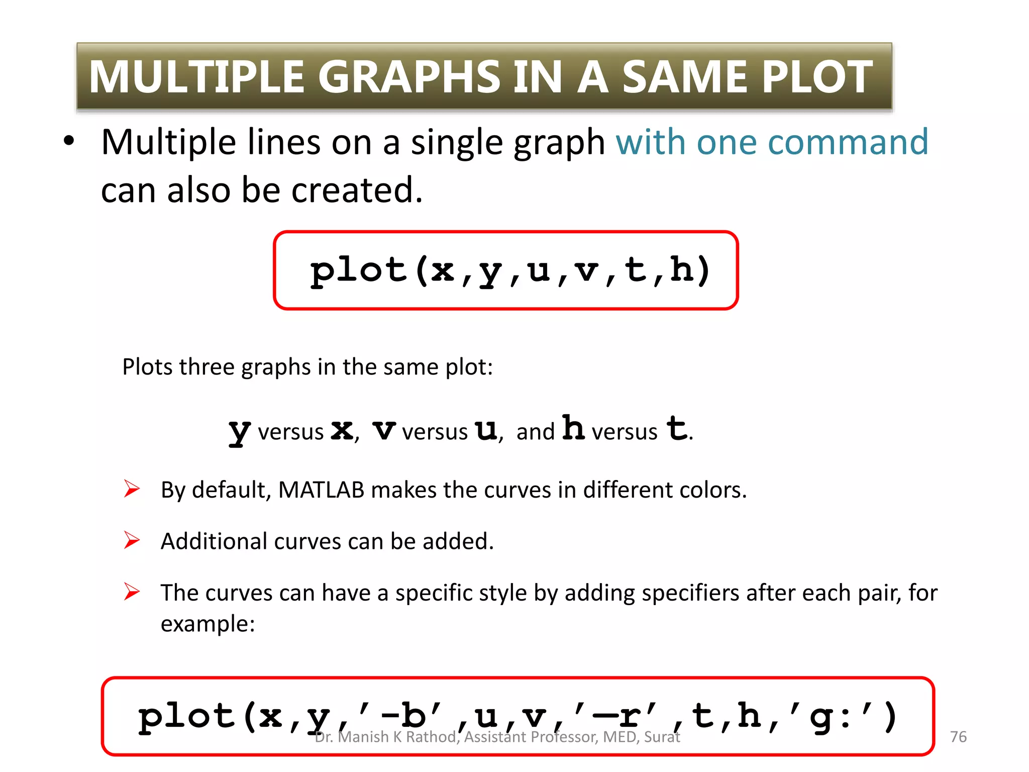
MULTIPLE GRAPHS IN A SAME PLOT
Dr. Manish K Rathod, Assistant Professor, MED, Surat 77](https://image.slidesharecdn.com/gettingstartmatlabbvm1-221215061824-4faa6455/75/Getting_Start_MATLAB_BVM1-pptx-77-2048.jpg)
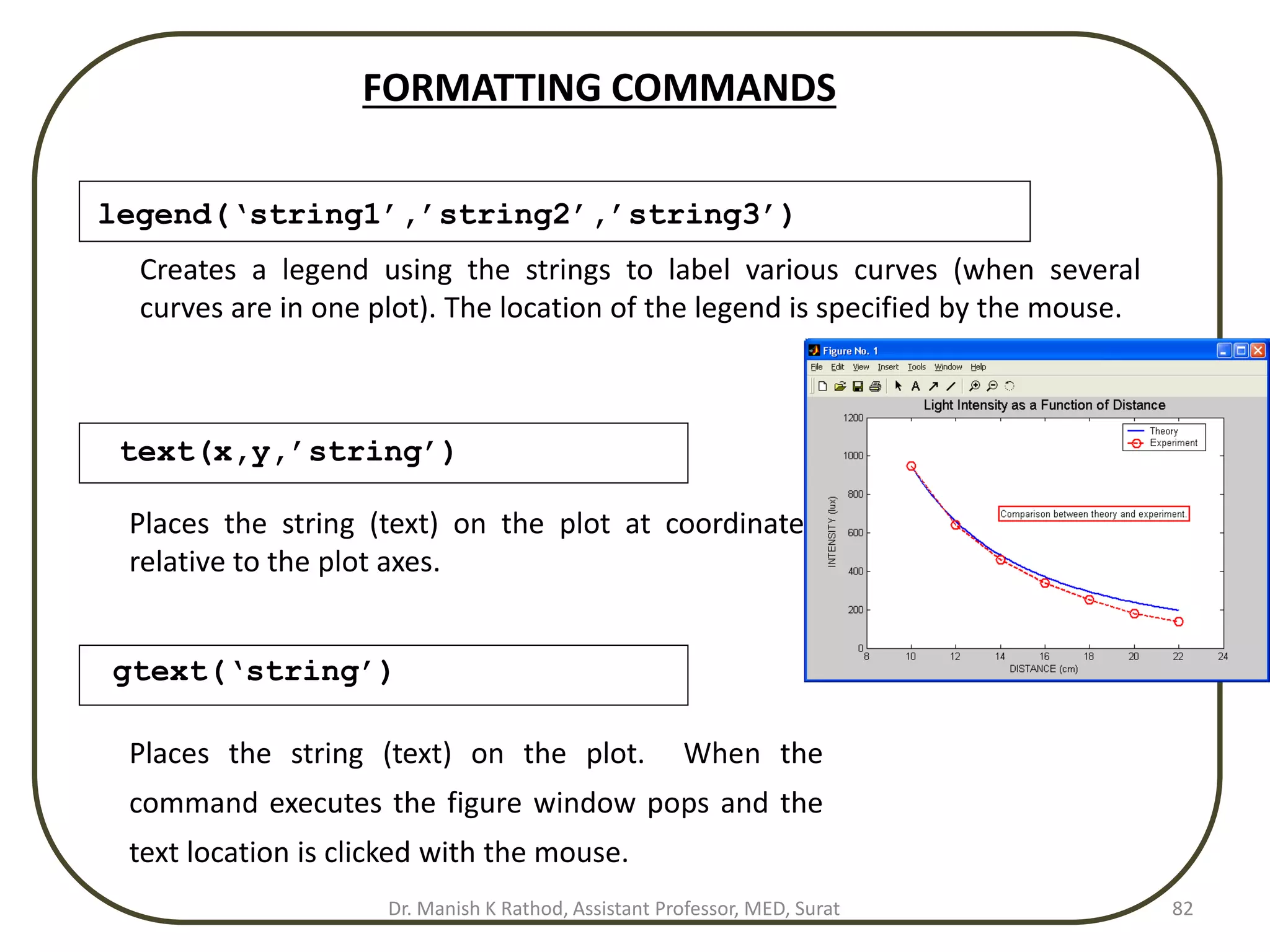
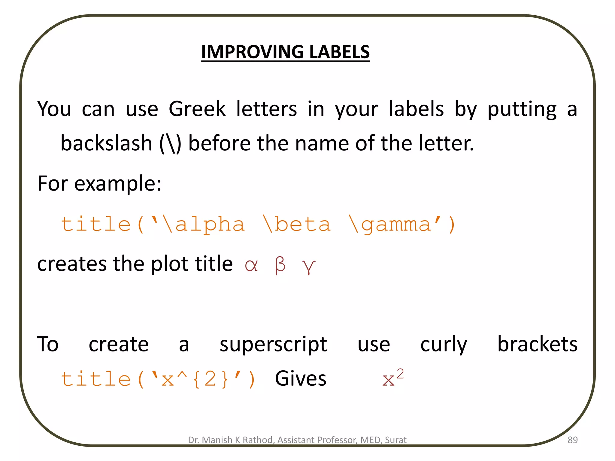
![FORMATTING COMMANDS
title(‘string’)
Adds the string as a title at the top of the plot.
xlabel(‘string’)
Adds the string as a label to the x-axis.
ylabel(‘string’)
Adds the string as a label to the y-axis.
axis([xmin xmax ymin ymax])
Sets the minimum and maximum limits of the x- and y-axes.
Dr. Manish K Rathod, Assistant Professor, MED, Surat 81](https://image.slidesharecdn.com/gettingstartmatlabbvm1-221215061824-4faa6455/75/Getting_Start_MATLAB_BVM1-pptx-81-2048.jpg)
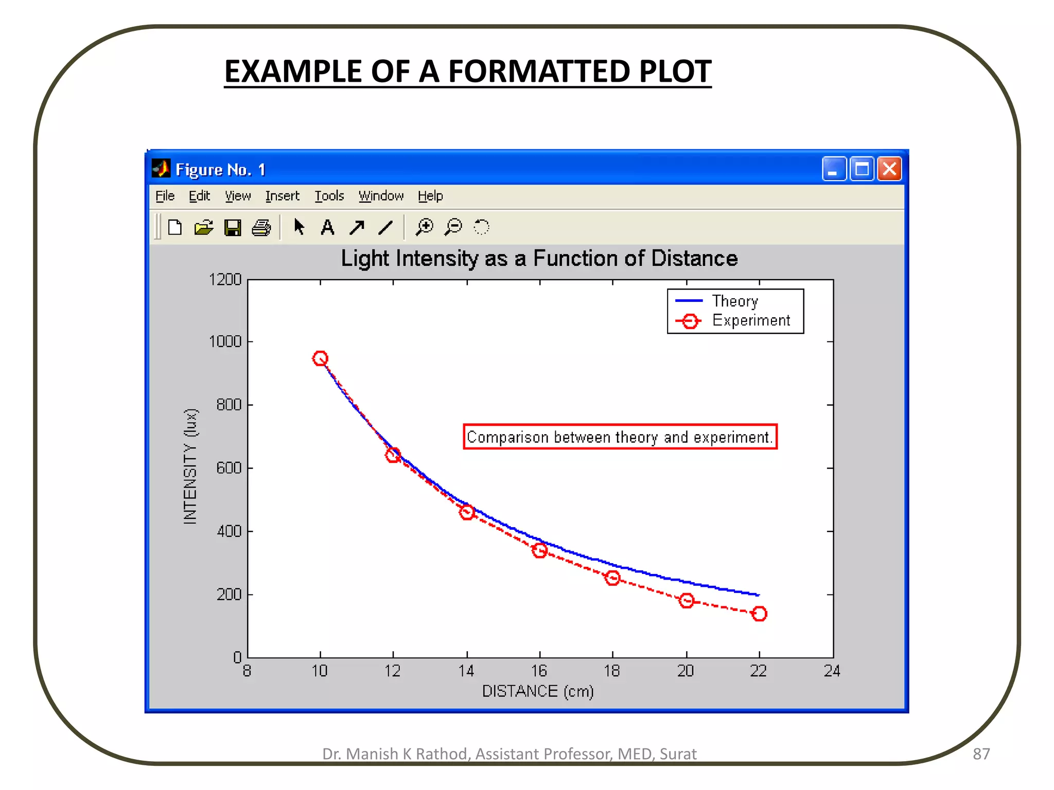
![EXAMPLE OF A FORMATTED PLOT
Below is a script file of the formatted light intensity plot
x=[10:0.1:22];
y=95000./x.^2;
xd=[10:2:22];
yd=[950 640 460 340 250 180 140];
plot(x,y,'-','LineWidth',1.0)
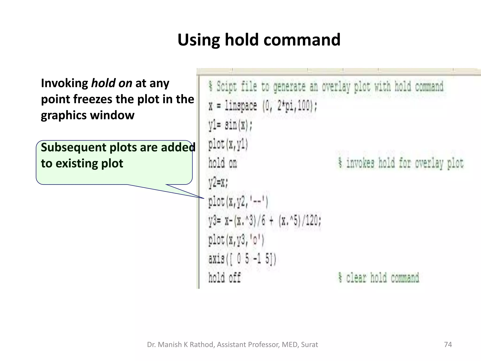
hold on
plot(xd,yd,'ro--',‘LineWidth',1.0,'markersize',10)
hold off
Creating a vector with light
intensity from data.
Creating a vector with coordinates of data points.
Creating vector x for plotting the theoretical curve.
Creating vector y for plotting the theoretical curve.
Dr. Manish K Rathod, Assistant Professor, MED, Surat 85](https://image.slidesharecdn.com/gettingstartmatlabbvm1-221215061824-4faa6455/75/Getting_Start_MATLAB_BVM1-pptx-85-2048.jpg)
![EXAMPLE OF A FORMATTED PLOT
Formatting of the light intensity plot (cont.)
xlabel('DISTANCE (cm)')
ylabel('INTENSITY (lux)')
title('fontname{Arial}Light Intensity as a Function of Distance','FontSize',14)
axis([8 24 0 1200])
text(14,700,'Comparison between theory and
experiment.','EdgeColor','r','LineWidth',2)
legend('Theory','Experiment',0)
Creating text.
Creating a legend.
Title for the plot.
Setting limits of the axes.
Labels for the axes.
The plot that is obtained is shown again in the next slide.
Dr. Manish K Rathod, Assistant Professor, MED, Surat 86](https://image.slidesharecdn.com/gettingstartmatlabbvm1-221215061824-4faa6455/75/Getting_Start_MATLAB_BVM1-pptx-86-2048.jpg)


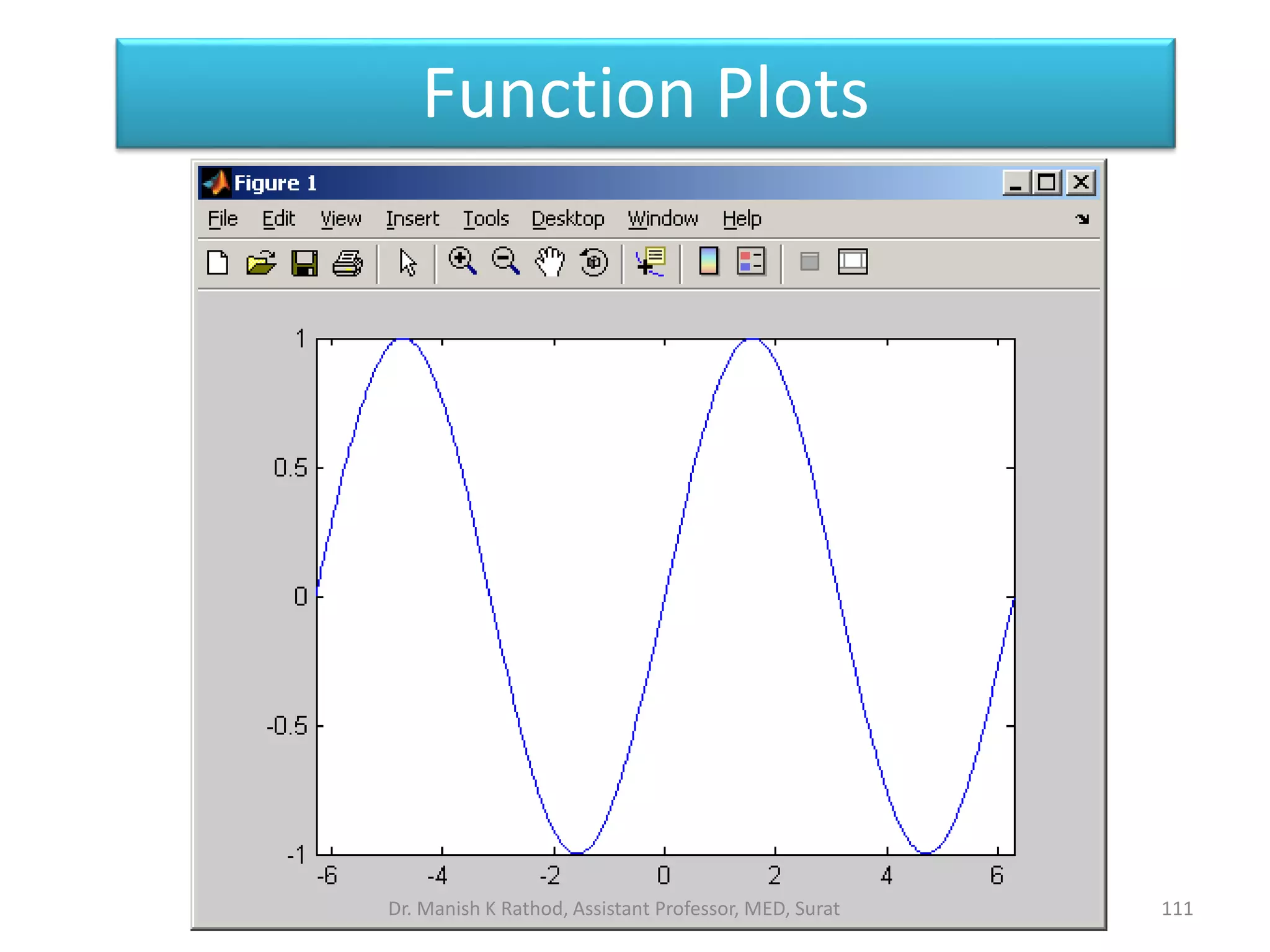
![Function Plots
110
• Function plots allow you to use a function as
input to a plot command, instead of a set of
ordered pairs of x-y values
• fplot('sin(x)',[-2*pi,2*pi])
function input as a
string
range of the independent
variable – in this case x
Dr. Manish K Rathod, Assistant Professor, MED, Surat](https://image.slidesharecdn.com/gettingstartmatlabbvm1-221215061824-4faa6455/75/Getting_Start_MATLAB_BVM1-pptx-110-2048.jpg)
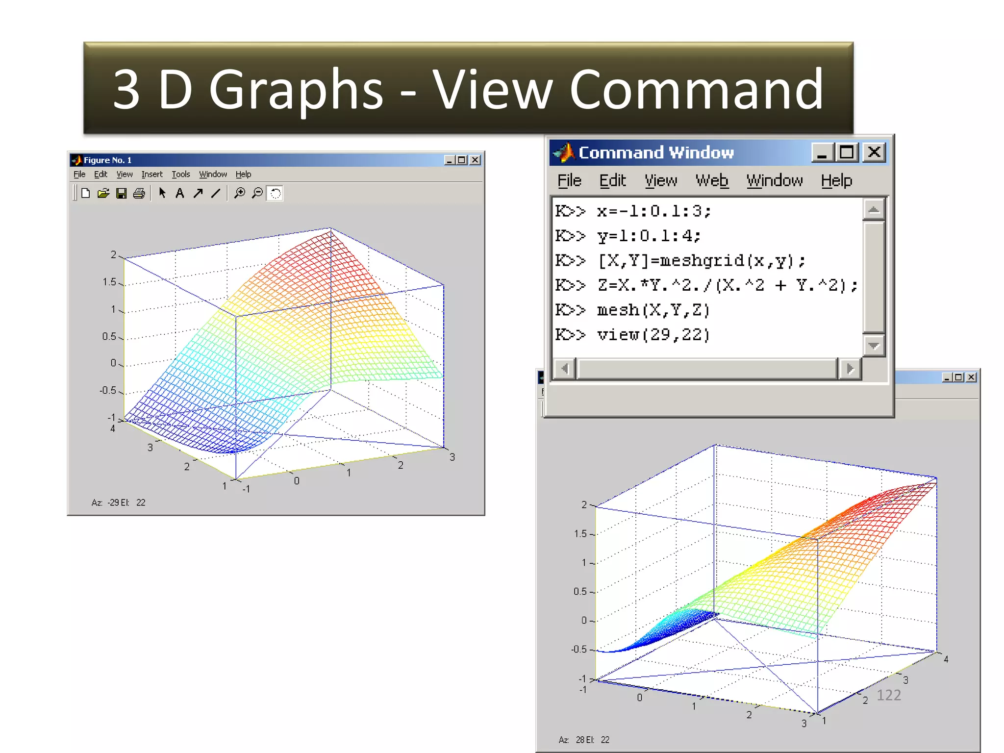
![• Controls the direction from which the plot is
viewed.
• Done by specifying a direction in terms of
azimuth and elevation angles.
• View (az,el) or view([az,el])
Angle in the x-y plane measured
relative to the negative y axis
direction and positive in counter
clockwise direction
Angle of elevation from
x-y plane.
3 D Graphs - View Command
Dr. Manish K Rathod, Assistant Professor, MED, Surat 121](https://image.slidesharecdn.com/gettingstartmatlabbvm1-221215061824-4faa6455/75/Getting_Start_MATLAB_BVM1-pptx-121-2048.jpg)