This document discusses data structures and algorithms. It provides grading schemes for theory and lab components. It acknowledges reference sources used to prepare the lecture. Key points covered include: what data structures are and why they are important for organizing data efficiently; characteristics of good data structures like time and space complexity; definitions of algorithms and examples like searching and sorting; and algorithmic notations used to describe processes like linear and binary search of arrays.

1. Lecture No.01
Data Structures and
Algorithms
Rabbia mahum, UET Taxila

2. Grading Theory
 Mid Term 25%
 Final 50%
 Programming Assignments 10%
 Surprise Quiz's 05%
 Project 10%

3. Grading Lab
 Mid Term 25%
 Final 50%
 Programming Project 20%
 Presentation and viva voca 05%

4. Acknowledgement
This Lecture has been prepared from your Reference Course Book titled as
“Data Structure” by Schaum Series.
Other source includes tutorialpoint page and google pages
4

5. What is Data Structures
 Data Structures are the programmatic way of storing data so that
data can be used efficiently.
 Almost every enterprise application uses various types of data
structures in one or the other way.
5

6. Why to Learn Data Structure and
Algorithms?
 As applications are getting complex and data rich, there are three
common problems that applications face now-a-days.
1. Data Search
2. Processor speed
3. Multiple requests
6

7. Why to Learn Data Structure and
Algorithms?
 Data Search − Consider an inventory of 1 million(106) items of a
store. If the application is to search an item, it has to search an item
in 1 million(106) items every time slowing down the search. As data
grows, search will become slower.
7

8. Why to Learn Data Structure and
Algorithms?
 Processor speed − Processor speed although being very high, falls
limited if the data grows to billion records.
 Multiple requests − As thousands of users can search data
simultaneously on a web server, even the fast server fails while
searching the data.
8

9. Why to Learn Data Structure and
Algorithms?
 To solve these mentioned problems, data structures come to rescue.
 Data can be organized in a data structure in such a way that all items
may not be required to be searched, and the required data can be
searched almost instantly.
9

10. Data Structure: Foundation terms
 Interface − Each data structure has an interface. Interface represents
the set of operations that a data structure supports. An interface only
provides the list of supported operations, type of parameters they can
accept and return type of these operations.
10

11. Data Structure: Foundation terms
 Implementation − Implementation provides the internal
representation of a data structure.
 Implementation also provides the definition of the algorithms used in
the operations of the data structure.
11

12. Characteristics of a Data Structure
1. Correctness − Data structure implementation
should implement its interface correctly.
2. Time Complexity − Running time or the execution
time of operations of data structure must be as
small as possible.
3. Space Complexity − Memory usage of a data
structure operation should be as little as possible.
12

13. What is an Algorithm?
 The word algorithm comes from the name of a Persian author, Abu Ja’far
Mohammed ibn Musa al Khowarizmi (c. 825 A.O.) who wrote a textbook on
mathematics.
 An examination of the latest edition of Webster's dictionary defines its
meaning as "any special method of solving a certain kind of problem.
13

14. Definition of “Algorithm”
 An Algorithm, intuitively speaking, is a finite step-by-step list of well
defined instructions for solving a particular problem.
 An algorithm is a clearly specified set of simple instructions to be
followed to solve a problem.
14

15. Definition of “Algorithm”
 Algorithms are generally created independent of underlying languages,
i.e. an algorithm can be implemented in more than one programming
language.
15

16. Definition of “Algorithm”
 From the data structure point of view, following
are some important categories of algorithms −
1. Search − Algorithm to search an item in a data
structure.
2. Sort − Algorithm to sort items in a certain order.
3. Insert − Algorithm to insert item in a data structure.
4. Update − Algorithm to update an existing item in a data
structure.
5. Delete − Algorithm to delete an existing item from a
data structure.
16

17. Properties or Constraints
 For example, each operation must be definite, meaning that it must
be perfectly clear what should be done.
 Directions such as "compute 5/0" or "add 6 or 7 to x" are not permitted
because it is not clear what the result is or which of the two possibilities
should be done.
17

18. Properties or Constraints
 Another important property each operation should have is that it be
effective; each step must be such that it can, at least in principle, be
done by a person using pencil and paper in a finite amount of time.
 Arithmetic operations on integer is an effective while on some real
numbers its not……
18

19. Properties or Constraints
 An algorithm produces one or more outputs and may have zero or
more inputs which are externally supplied.
 Another important criterion we will assume about algorithms is that
they terminate after a finite number of operations.
19

20. Algorithmic Notations
 In coming slides you will learn the format that is used to present
algorithms throughout this course. This is best describes by means of an
example.
 Example: An array DATA of numerical values is in memory. We want to
find the location LOC and the value MAX of the largest element of DATA.
20

21. Algorithmic Notations
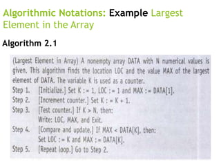
 Initially begin with LOC = 1 and MAX = DATA
[1]. Then compare MAX with each successive
element DATA[K] of DATA.
 If DATA[K] exceeds MAX then update LOC and
MAX so that LOC = K and MAX = DATA [K].
 The final values appearing in LOC and MAX give
the location and value of the largest element
of DATA. 21

22. Algorithmic Notations: Example Largest
Element in the Array
Algorithm 2.1

23. Algorithmic Notations: Example Largest
Element in the Array
Flow Chart

24. Algorithmic Notations: The Solution of the
Quadratic Equation

25. Algorithmic Notations: The Solution of the
Quadratic Equation
 The quantity D = b2 – 4ac is called the
discriminant of the equation. If D is negative,
then there are no real solutions.
 If D = 0, then there is only one (double) real
solution , x = -b/2a
 If D is positive, the formula gives the two
distinct real solutions.

26. Algorithmic Notations: The Solution of the
Quadratic Equation
Algorithm 2.3

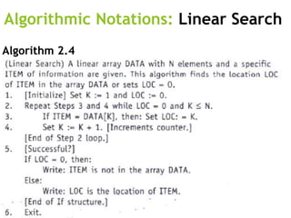
27. Algorithmic Notations: Linear Search
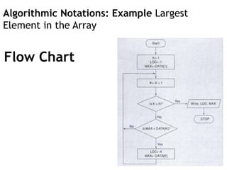
 Suppose a linear array DATA contains n elements,
and suppose a specific ITEM of information is given.
We want either to find the location LOC of item in
the array DATA, or to send some message, such as
LOC = 0, to indicate that ITEM is not in the DATA.
 The linear search algorithm solves this problem by
comparing ITEM, one by one, with each element in
DATA. That is we compare ITEM with DATA[1],
DATA[2], and so on, until we find LOC such that ITEM
= DATA [LOC].
Algorithm 2.4

28. Algorithmic Notations: Linear Search
Algorithm 2.4

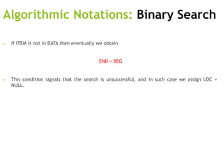
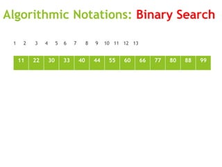
29. Algorithmic Notations: Binary Search
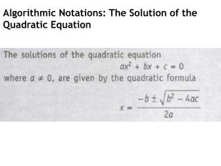
 During each stage of binary search algorithm our search
for ITEM is reduced to a segment of elements of DATA
 The BEG and END denote respectively the beginning and
end location of segment under consideration. Where
BEG = 1 or LB and END = n or UB
 The Algorithm compares ITEM with the middle element
DATA[MID] of segment where MID is obtained by
MID = INT (BEG + END ) /2

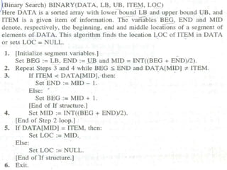
30. Algorithmic Notations: Binary Search
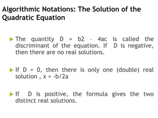
 If DATA [MID] = ITEM then search is successful and we
set LOC = MID, otherwise a new segment of DATA is
obtained as follow
 A) If ITEM < DATA [MID] then ITEM can appear on left
side of segment
 DATA [BEG] , DATA [BEG+1] … DATA[MID -1]
B) If ITEM > DATA [MID] then ITEM can appear in right half of the
segment
 DATA [MID] , DATA [MID+1] … DATA[END]

31. Algorithmic Notations: Binary Search
• If ITEM is not in DATA then eventually we obtain
END < BEG
• This condition signals that the search is unsuccessful, and in such case we assign LOC =
NULL.

32. Algorithmic Notations: Binary Search
1 2 3 4 5 6 7 8 9 10 11 12 13
11 22 30 33 40 44 55 60 66 77 80 88 99

33. Algorithmic Notations: Linear Search
Algorithm 2.4